A Deep Learning Model Integrating EEMD and GRU for Air Quality Index Forecasting

Abstract

Accurate prediction of the air quality index (AQI) is essential for environmental monitoring and sustainable urban planning. With rising pollution from industrialization and urbanization, particularly from fine particulate matter (PM_2.5, PM₁₀), nitrogen dioxide (NO₂), and ozone (O₃), robust forecasting tools are needed to support timely public health interventions. This study proposes a hybrid deep learning framework that combines empirical mode decomposition (EMD) and ensemble empirical mode decomposition (EEMD) with two recurrent neural network architectures: long short-term memory (LSTM) and gated recurrent unit (GRU). A comprehensive dataset from Xitun District, Taichung City—including AQI and 18 pollutant and meteorological variables—was used to train and evaluate the models. Model performance was assessed using root mean square error, mean absolute error, mean absolute percentage error, and the coefficient of determination. Both LSTM and GRU models effectively capture the temporal patterns of air quality data, outperforming traditional methods. Among all configurations, the EEMD-GRU model delivered the highest prediction accuracy, demonstrating strong capability in modeling high-dimensional and nonlinear environmental data. Furthermore, the incorporation of decomposition techniques significantly reduced prediction error across all models. These findings highlight the effectiveness of hybrid deep learning approaches for modeling complex environmental time series. The results further demonstrate their practical value in air quality management and early-warning systems.

1. Introduction

Air pollution is a critical environmental challenge with far-reaching consequences for public health, ecological integrity, and socio-economic development [1,2]. As urbanization and industrialization intensify worldwide, the burden of airborne pollutants has become increasingly evident in both developed and developing regions. Pollutants such as fine particulate matter (PM_2.5, PM₁₀), nitrogen dioxide (NO₂), and ground-level ozone (O₃) contribute to a broad spectrum of health issues, ranging from respiratory and cardiovascular diseases to premature mortality [3,4,5]. These impacts are particularly severe for vulnerable groups, including children, the elderly, and those with preexisting health conditions. In addition to human health, air pollution affects agricultural yields [6], accelerates the deterioration of infrastructure [7,8], and contributes to climate change by altering atmospheric composition [9]. Addressing these multifaceted impacts requires not only mitigation strategies but also reliable tools for air quality forecasting to support early interventions and sustainable policy decisions.

Taiwan serves as a representative case of the broader challenges posed by air pollution. As a subtropical island with a dense population and extensive industrial and transportation activities, it faces persistent air quality issues that vary across regions and seasons [10,11]. In urban and industrial hubs such as Xitun District in Taichung City, air pollution stems from multiple sources, including vehicular emissions, industrial processes, and seasonal monsoonal winds that transport transboundary pollutants. During the winter months, atmospheric conditions—particularly temperature inversions—often trap pollutants near the surface, resulting in smog events and elevated public health risks [12]. Residents in these areas experience frequent fluctuations in air quality, creating a strong demand for accurate and timely forecasting systems. While traditional methods such as linear regression and autoregressive models have been applied to this task, they often fail to capture the nonlinear and dynamic characteristics of air pollution data [13]. Even classical machine learning algorithms—such as support vector machines (SVM) and random forests (RF)—though more flexible, struggle to model long-term temporal dependencies and the high variability of environmental conditions [14,15].

To address the limitations of both traditional and classical machine learning approaches, deep learning has emerged in recent years as a powerful alternative for environmental time series forecasting. Recurrent neural networks (RNNs)—particularly long short-term memory (LSTM) and gated recurrent unit (GRU) architectures—are well-suited to capturing complex temporal dependencies in data [16,17]. These models can learn long-range patterns and nonlinear relationships without extensive manual feature engineering, making them especially suitable for air quality index (AQI) prediction [17,18]. However, one of the primary challenges in applying deep learning to real-world environmental datasets lies in the presence of noise, missing values, and non-stationary behavior, which can reduce model performance. To mitigate these issues, signal decomposition techniques such as empirical mode decomposition (EMD) and its improved variant, ensemble empirical mode decomposition (EEMD), have been employed to preprocess time series inputs [18]. These methods decompose complex signals into intrinsic mode function (IMF), enabling the models to learn from denoised and smoothed data representations. Despite these advancements, several research gaps remain. First, there is limited comparative analysis of how different decomposition methods, when integrated with deep learning architectures, affect AQI prediction accuracy [19]. Second, many existing studies rely on a limited number of pollutant variables, potentially omitting important environmental factors. Finally, while hybrid models have been proposed, few studies evaluate their robustness and generalizability using real-world multivariate air quality data from high-density urban environments.

To address existing gaps in air quality forecasting, this study investigates the following research questions:

• Among long short-term memory (LSTM) and gated recurrent unit (GRU) architectures integrated with empirical mode decomposition (EMD) and ensemble empirical mode decomposition (EEMD), which hybrid model yields the highest predictive accuracy for air quality index (AQI) forecasting?
• To what extent can deep learning models effectively process high-dimensional, nonlinear environmental datasets?
• How can improved model accuracy support government agencies and enterprises in enhancing air pollution monitoring and control strategies?
• Can accurate air quality index (AQI) predictions improve public health outcomes by enabling timely responses to pollution events?

To this end, we propose and evaluate a hybrid framework that combines EMD and EEMD with both LSTM and GRU models. Using a comprehensive dataset from Xitun District, including AQI and 18 pollutant and meteorological variables, we train and test various model configurations. Forecasting performance is evaluated using standard metrics: root mean squared error (RMSE), mean absolute error (MAE), mean absolute percentage error (MAPE), and the coefficient of determination (R²). The findings of this study demonstrate that integrating signal decomposition techniques with deep learning models significantly improves AQI forecasting performance. Among all configurations, the GRU model combined with EEMD model achieved the highest predictive accuracy, outperforming other hybrid models in terms of RMSE, MAE, MAPE, and R². Results show that integrating signal decomposition significantly enhances AQI prediction. The EEMD-GRU model achieved the highest accuracy, outperforming all alternatives across metrics. The EEMD preprocessing step effectively reduced data noise and improved stability, while the GRU model benefited from a simpler architecture and faster convergence compared to LSTM. By incorporating a wide range of environmental features, the proposed model captures intricate interactions influencing air quality in densely populated areas. These findings affirm the effectiveness of combining deep learning with signal decomposition for real-time AQI forecasting and suggest meaningful applications in public health alert systems and environmental policy planning. In addition, this study integrates automated hyperparameter optimization (Optuna) and statistical validation to further enhance robustness and ensure the reliability of the results.

The remainder of this paper is organized as follows: Section 2 describes the study area and data sources. Section 3 outlines the proposed methodology. Section 4 presents the implementation and results. Section 5 concludes the paper and discusses future research directions.

2. Study Area and Data Description

2.1. Air Quality in Taiwan

Air quality is a major global concern, intersecting environmental science and public health. According to the World Health Organization (WHO), 99% of the global population breathes air that exceeds recommended pollution limits, with the highest exposures in low- and middle-income countries (LMICs) [5]. Ambient air pollution—driven by fine particulate matter and toxic gase8—contributes to major non-communicable diseases, including strokes, cardiovascular conditions, and respiratory illnesses. Additionally, 2.6 billion people are exposed to hazardous indoor air pollution from inefficient stoves and polluting fuels such as biomass and coal. To support public health communication, the air quality index (AQI) simplifies pollutant concentrations into a single, interpretable score [20,21], incorporating pollutants such as NO₂, Carbon Monoxide (CO), Carbon Dioxide (CO₂), O₃, Sulfur Dioxide (SO₂), PM_2.5, and PM₁₀ [22].

In Taiwan, the Ministry of Environment’s Air Quality Monitoring Network provides comprehensive surveillance, with stations placed based on emissions, meteorology, and pollutant distribution. The network includes 61 general, 6 traffic, 5 industrial, 2 national park, and 5 background stations, along with special-purpose sites. Effective 1 January 2025, Taiwan adopted revised AQI thresholds aligned with international standards, introducing a six-tier system from “Good” to “Hazardous” [23]. Table S1 in supplementary material outlines the revised categories and health guidelines. The system provides clearer risk communication and targeted recommendations for vulnerable groups, reflecting Taiwan’s commitment to sustainable air quality governance and public health protection.

2.2. Application of Deep Learning in Air Quality Prediction

Air pollution continues to pose serious risks to public health and environmental sustainability, prompting the need for accurate AQI forecasting. Traditional models often fail to handle the nonlinear, high-dimensional nature of AQI data. In contrast, deep learning models—powered by advances in computational capabilities and large-scale environmental datasets—have shown strong potential in capturing complex spatiotemporal patterns. Recent research has explored a range of deep learning and hybrid approaches. Wang et al. [24] developed a fuzzy time series-based early warning system, demonstrating robust performance in terms of prediction accuracy and stability. Wu and Lin [19] proposed a hybrid model integrating sub-decomposition (SD), LSTM, least squares support vector machine (LSSVM), and bat algorithm (BA), achieving notable accuracy in AQI classification. Janarthanan et al. [25] compared support vector regression (SVR) and LSTM models and highlighted their practical applications in urban planning, such as optimizing traffic flow and identifying pollution hotspots. Similarly, Du et al. [26] combined one-dimensional convolutional neural networks (1D-CNN) with bidirectional long short-term memory (Bi-LSTM) to capture multivariate dependencies, significantly outperforming shallow and conventional deep models. Espinosa et al. [27] evaluated multiple models—1D-CNN, GRU, LSTM, RF, lasso regression, and SVR—and found them effective for reliable 24 h AQI forecasting. Sarkar et al. [28] introduced a hybrid LSTM-GRU model that outperformed traditional models like SVM and k-nearest neighbors (KNN) in terms of both accuracy and stability.

Among these architectures, LSTM and GRU are widely adopted for time series forecasting due to their ability to handle vanishing gradients and model long-term dependencies. Shewalkar [29] noted that LSTM performs better in speech-related tasks, whereas GRU offers comparable accuracy with faster training, ideal for resource-constrained settings. Gao et al. [30] reported both models outperforming traditional ANNs in runoff prediction, with GRU showing higher efficiency. Yang et al. [31] found GRU superior to LSTM on smaller datasets and longer inputs based on multiple performance metrics. Gao et al. [32] further demonstrated that GRU excels in short-term traffic forecasts, while LSTM performs better with larger datasets and long-term predictions. Collectively, these studies underscore the effectiveness and flexibility of deep learning approaches in AQI prediction. As data availability and model architectures continue to evolve, more accurate, robust, and interpretable forecasting tools are expected to play an increasingly important role in environmental policy-making and public health planning.

2.3. Data Collection and Variable Selection

Air quality forecasting models rely heavily on comprehensive datasets provided by government agencies, monitoring stations, and research institutions. These datasets typically include measurements of major air pollutants such as PM_2.5, PM₁₀, NO₂, CO, SO₂, and O₃, which are recognized for their health impacts and environmental relevance [19,24,28]. Among these, PM_2.5 often receives particular emphasis due to its ability to penetrate deep into the respiratory system. For instance, Wang et al. [24] focused on PM_2.5, PM₁₀, and SO₂, reflecting concern over pollutants linked to respiratory diseases and industrial emissions.

To capture the full dynamics of air quality, recent studies have increasingly incorporated meteorological variables such as temperature, relative humidity, wind speed and direction, atmospheric pressure, and sunshine duration [26,27]. These environmental factors influence the formation and dispersion of air pollutants and are essential for improving model accuracy. In parallel, some researchers have broadened their input variables to include traffic-related metrics like vehicle flow and congestion levels, especially in urban areas where road transport is a dominant pollution source [27]. Beyond physical and chemical variables, there is also growing interest in examining how specific events impact air quality. For example, Janarthanan et al. [25] incorporated volatile organic compounds (VOCs) to better account for secondary pollutant formation, while Agarwal et al. [33] used data from COVID-19 lockdown periods to assess how reduced human activity altered emission patterns. These studies highlight the value of context-specific data in uncovering pollution dynamics.

Data is typically collected over several months or years, with hourly or daily resolution, offering rich temporal detail for model development. Urban areas with high population density and industrial or vehicular activity are common study sites due to their elevated pollution variability and public health risks. Ultimately, the selection of variables depends on the study’s objectives, local emission sources, and desired model interpretability. As summarized in Table S2, recent study increasingly integrates both pollutant and meteorological variables to enhance predictive performance and environmental insight.

3. Methodology

This study selects Xitun District, Taichung City, Taiwan, as the research site due to its high population density, industrial presence, and traffic-related emissions. As home to the Central Taiwan Science Park and major transportation routes, Xitun experiences frequent air quality fluctuations [34], making it a representative urban area for AQI forecasting. The district’s established environmental monitoring stations provide high-quality, high-frequency data suitable for time series modeling. Accurate predictions in this context can help residents take preventive health measures and support government and industry efforts in formulating effective pollution control strategies.

3.1. Data Sources and Processing

3.1.1. Air Quality Index and Meteorological Data Collection

The air quality index (AQI) data used in this study were obtained from Taiwans Air Quality Monitoring Network, managed by the Ministry of Environment. The dataset covers Xitun District in Taichung City and spans the period from 1 January 2021 to 31 December 2023. The raw data were stored in Excel format, with each entry containing the following information:

• Monitoring station name: The specific location where air quality measurements were recorded.
• AQI value: The hourly air quality index, indicating the level of air pollution at a given time.
• Date and time (datacreationdate): The timestamp of data generation, accurate to the hour.

Meteorological parameters used in this study are listed in

Table 1. Meteorological parameters.

No	Parameters	Units
1	AMB_TEMP (Ambient temperature)	°C
2	CH4 (Methane concentration)	ppm
3	CO (Carbon monoxide concentration)	ppm
4	NMHC (Non-methane hydrocarbons concentration)	ppm
5	NO (Nitric oxide concentration)	ppb
6	NO2 (Nitrogen dioxide concentration)	ppb
7	NOx (Total nitrogen oxides concentration)	ppb
8	O3 (Ozone concentration)	ppb
9	PM10 (Particulate matter concentration)	μg/m3
10	PM2.5 (Fine particulate matter concentration)	μg/m3
11	RAINFALL (Rainfall)	mm
12	RH (Relative humidity)	%
13	SO2 (Sulfur dioxide concentration)	ppb
14	THC (Total hydrocarbons concentration)	ppb
15	WD_HR (Horizontal component of wind speed)	m/s
16	WIND_DIREC (Wind direction)	degrees
17	WIND_SPEED (Wind speed)	m/s
18	WS_HR (Vertical component of wind speed)	m/s

. To analyze daily variations in air quality, the original hourly AQI data were aggregated into daily averages. The preprocessing included standardizing the timestamp format, extracting the date component, and grouping the data by day to calculate average AQI values. These steps were implemented using Python’s pandas library (version 2.2.2). The resulting daily dataset was exported in CSV format for use in subsequent modeling and analysis.

3.1.2. Data Pre-Processing

Before model development, several pre-processing steps were conducted to ensure data consistency, accuracy, and suitability for analysis:

• Missing value imputation: To handle missing values, linear interpolation—a standard method for time series data—was used. It estimates missing points based on adjacent values, assuming a smooth trend, as shown in the equation below:

  $$x_t\mathrm{ }=\mathrm{ }{x}_{t-1}+{\displaystyle \frac{x_{t+1}-x_{t-1}}{t+1-\left(t-1\right)}}\times \left(t-\left(t-1\right)\right)$$

  (1)

  where $x_t$ is the imputed value at time t, and $x_{t-1}$ and $x_{t+1}$ are the known values at times $t-1$ and $t+1$, respectively.
• Normalization and standardization: To address feature scale differences, Min-Max normalization was applied to deep learning models, rescaling inputs to the [0, 1] range:

  $$X^{\prime }\mathrm{ }=\mathrm{ }{\displaystyle \frac{X-min\left(X\right)}{max\left(X\right)-min\left(X\right)}}$$

  (2)

  where $X^{\prime }$ is the normalized value. In contrast, Z-score standardization was used for models sensitive to feature variance, ensuring a mean of zero and standard deviation of one:

  $$\mathrm{Z}\mathrm{ }=\mathrm{ }{\displaystyle \frac{X-\mu }{\sigma }}$$

  (3)

  where $\mu$ and $\sigma$ represent the mean and standard deviation of feature $X$, respectively.
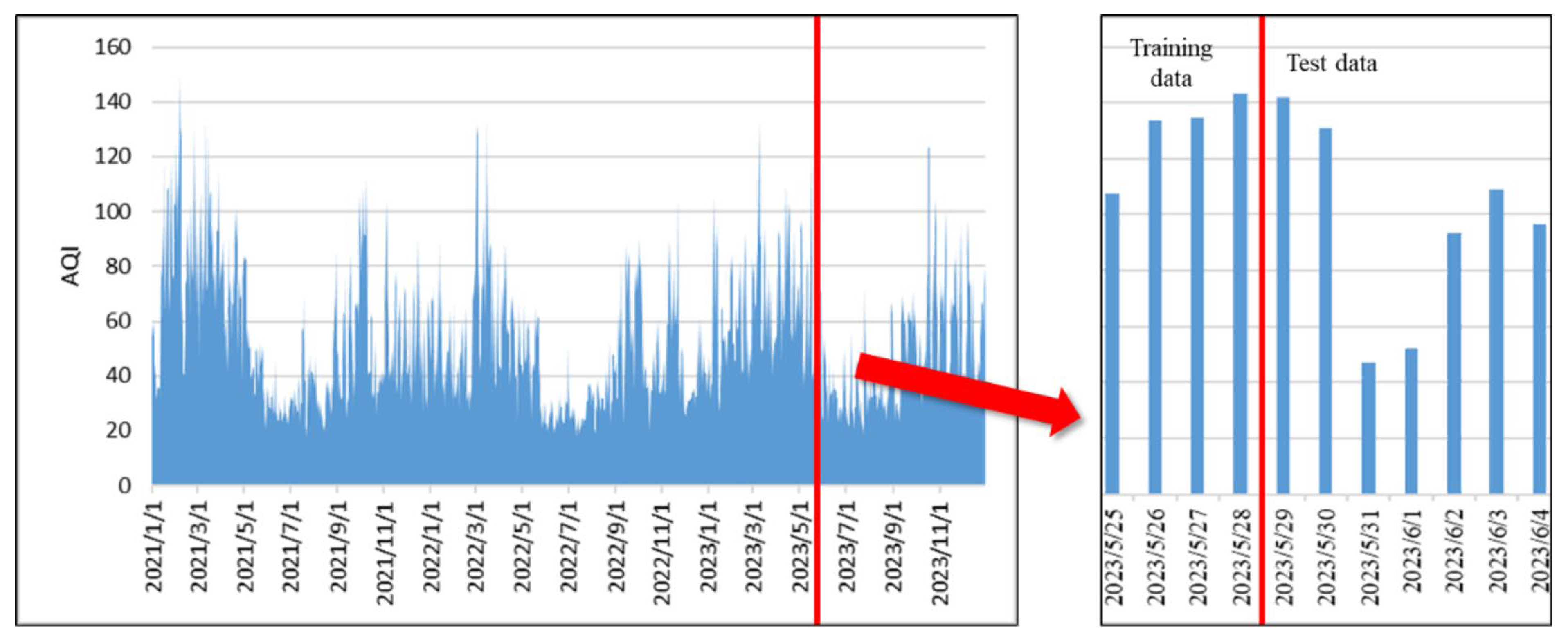
• Data splitting: The dataset was split into training and testing sets in an 80:20 ratio to evaluate model performance on unseen data and reduce overfitting. The entire AQI time series used for model development is illustrated in Figure 1, which highlights both the full dataset (left) and the partitioning into training and testing sets (right), clearly marked by the red vertical line

3.1.3. Gray Relational Analysis

Gray relational analysis (GRA) is a widely used method for quantifying the degree of association between variables, particularly effective in cases with limited data or high uncertainty. It is commonly applied in multi-factor analysis to identify variables that most strongly influence a target metric. In this study, GRA is applied to assess the correlation between various meteorological and pollutant variables and AQI in Xitun District. The analysis involves the following steps:

• Research data: Environmental monitoring data from 2021 to 2023 were obtained from the Taiwan Air Quality Monitoring Network, including variables such as AQI, Ambient temperature (AMB_TEMP), CH₄, CO, Non-methane hydrocarbons concentration (NMHC), NO, NO₂, NO_x, O₃, PM₁₀, PM_2.5, RAINFALL, Relative humidity (RH), SO₂, Total hydrocarbons concentration (THC), Horizontal component of wind speed (WD_HR), Wind direction (WIND_DIREC), Wind speed (WIND_SPEED), and Vertical component of wind speed (WS_HR).
• Missing value imputation: Linear interpolation (as described in the data pre-processing section) was used to fill missing values, ensuring temporal continuity.
• Data standardization: Variables were standardized using the Z-score method, consistent with the procedure outlined in the data pre-processing step.
• GRA computation: The procedure includes:

  (i)

  Gray relational coefficient: AQI is designated as the reference sequence ($X_0$), while the remaining variables serve as comparative sequences ($X_i$). The coefficient between AQI and each variable is calculated as:

  $${\xi }_i\mathrm{ }=\mathrm{ }{\displaystyle \frac{\underset{i,k}{\min }{∆}_i\left(k\right)+\rho \underset{i,k}{\max }{∆}_i\left(k\right)}{{∆}_i\left(k\right)+\rho \underset{i,k}{\max }{∆}_i\left(k\right)}}$$

  (4)

  where ${∆}_i\left(k\right)=\left|X_0\left(k\right)-X_i\left(k\right)\right|$ and $\rho$ is the distinguishing coefficient, typically set to 0.5.

  (ii)

  Average gray relational degree: The mean coefficient over all time points is computed as:

  $${\gamma }_i\mathrm{ }=\mathrm{ }{\displaystyle \frac{1}{n}}{\sum }_{k=\mathrm{ }1}^n{\xi }_i\left(k\right)$$

  (5)

  where ${\gamma }_i$ reflects the overall strength of the relationship between variable i and AQI.
• Result visualization: Variables are ranked based on ${\gamma }_i$ values to identify key influencers of AQI. A heatmap was also generated using Seaborn (version 0.13.2) to visually interpret the correlation patterns between AQI and other variables.

Although GRA provides a ranking of variable importance, all 18 variables were retained for model development. This decision was made to preserve potential interactions among meteorological and pollutant factors, which might be lost if only top-ranked features were selected. To further examine the effect of dimensionality reduction, we conducted preliminary experiments using principal component analysis (PCA). PCA transforms correlated variables into a smaller set of uncorrelated components while retaining most of the variance. The proportion of variance explained by the first eight components is summarized in

Table 2. Proportion of variance explained by each principal component.

Principal Component	Explained Variance Ratio
PC1	0.4388
PC2	0.2604
PC3	0.0880
PC4	0.0614
PC5	0.0320
PC6	0.0293
PC7	0.0257
PC8	0.0195

. While PCA effectively reduced redundancy, predictive performance under all thresholds remained lower than the baseline EEMD-GRU model without PCA. The detailed forecasting results of these PCA experiments are presented in Section 4.2.4.

3.2. Model Construction

3.2.1. Long Short-Term Memory

Long short-term memory (LSTM), proposed by Hochreiter and Schmidhuber [16], are a type of recurrent neural network designed to capture long-term dependencies and mitigate the vanishing gradient problem [35]. Through memory cells and gating mechanisms—namely forget, input, and output gates—LSTM regulate information flow across time steps, allowing them to retain relevant data and filter out noise. This makes them particularly effective in modeling sequential patterns such as seasonality and trends. LSTM have demonstrated success across various domains, including speech recognition [3], stock price forecasting [36], and image analysis [37]. In air quality forecasting, they are well-suited for learning complex dependencies in time series pollutant and meteorological data. The internal computation of an LSTM cell involves the following set of equations:

$$f_t\mathrm{ }=\mathrm{ }\sigma \left(W_f{x}_t+U_f{h}_{t-1}+b_f\right)$$

(6)

$$i_t\mathrm{ }=\mathrm{ }\sigma \left(W_i{x}_i+U_i{h}_{t-1}+b_i\right)$$

(7)

$${\tilde{c}}_t=tanh\left(W_c{x}_t+U_c{h}_{t-1}+b_c\right)$$

(8)

$$c_t=\mathrm{ }{f}_t○c_{t-1}+i_t○{\tilde{c}}_t$$

(9)

$$o_t\mathrm{ }=\mathrm{ }\sigma \left(W_o{x}_t+U_o{h}_{t-1}+b_o\right)$$

(10)

$$h_t\mathrm{ }=\mathrm{ }{o}_t\times tanh\left(c_t\right)$$

(11)

In these equations, $x_t$ is the input vector at time t, and $h_{t-1}$ is the hidden state from the previous step. The vectors $f_t$, $i_t$, and $o_t$ represent the outputs of the forget, input, and output gates, respectively, with the sigmoid activation function σ(⋅) mapping values to [0, 1]. The candidate memory content ${\tilde{c}}_t$, generated via the hyperbolic tangent function tanh(⋅), is used to update the internal cell state $c_t$, regulated by the gates. The final hidden state $h_t$ is computed from the activated cell state and output gate. Matrices $W_{*}$ and $U_{*}$ are trainable weights for the input and hidden state, and $b_{*}$ are the bias terms. The operator ∘ denotes the element-wise (Hadamard) product.

3.2.2. Gated Recurrent Unit

The gated recurrent unit (GRU), proposed by Chung et al. [17], is a streamlined alternative to LSTM that preserves the ability to model long-term dependencies while reducing computational complexity. Unlike LSTM, GRU does not employ a separate memory cell; instead, it integrates the memory function directly within its hidden state through two gating mechanisms: the reset gate and the update gate. The reset gate $r_t$ controls the degree to which the previous hidden state $h_{t-1}$ contributes to the current candidate activation. The update gate $z_t$ determines the proportion of the previous hidden state that is retained versus replaced by the new candidate ${\tilde{h}}_t$. These mechanisms allow the model to effectively balance short- and long-term dependencies in sequential data. GRU is particularly advantageous in air quality prediction tasks where model efficiency, faster training, and reduced overfitting are essential [31]—especially when working with noisy, multivariate environmental data. The computations within a GRU cell are expressed as follows:

$$r_t\mathrm{ }=\mathrm{ }\sigma \left(W_r·\left[h_{t-1},x_t\right]\right)$$

(12)

$$z_t\mathrm{ }=\mathrm{ }\sigma \left(W_z\left[h_{t-1},x_t\right]\right)$$

(13)

$$\mathrm{ }\mathrm{ }\mathrm{ }{h}_t=\mathrm{ }tanh\left(W_h\left[r_t\ast h_{t-1},x_t\right]\right)$$

(14)

$$h_t\mathrm{ }=\mathrm{ }\left(1-z_t\right)\ast h_{t-1}+z_t\ast h_t$$

(15)

$$y_t\mathrm{ }=\mathrm{ }\sigma \left(W_o·h_t\right)$$

(16)

Here, $x_t$ is the input, and $h_{t-1}$ is the previous hidden state, and [] denotes concatenation. The operator ∗ indicates element-wise multiplication. Due to its simpler design, GRU often trains faster and performs well on smaller datasets, offering a practical trade-off between complexity and accuracy. Previous studies (e.g., [29]) have shown GRU’s effectiveness across various forecasting tasks.

3.2.3. Empirical Mode Decomposition

Empirical mode decomposition (EMD) is a data-driven technique designed to decompose nonlinear and non-stationary signals into intrinsic mode function (IMF). Unlike Fourier or wavelet transforms, EMD does not require predefined basis functions, making it well-suited for complex environmental datasets such as AQI time series. In this study, EMD is employed to extract multi-scale temporal features from AQI data, facilitating more efficient learning in LSTM and GRU models. The EMD process involves the following steps:

• Extrema identification: Detect local maxima and minima from the original signal x(t).
• Envelope construction: Interpolate extrema using cubic splines to form upper and lower envelopes.
• Mean computation: Calculate the local mean m(t) as the average of the two envelopes.
• IMF extraction: Compute the candidate IMF via:

  $$\mathrm{h}\left(t\right)=x\left(t\right)-m\left(t\right)$$

  (17)

  and apply the sifting process until the resulting $\mathrm{h}\left(t\right)$ satisfies the IMF conditions: (1) the number of zero crossings and extrema differ at most by one, and (2) the mean envelope is approximately zero.
• Residue calculation: Subtract the IMF from the signal to compute the residue:

  $$\mathrm{ }\mathrm{ }\mathrm{ }\mathrm{ }\mathrm{r}\left(t\right)\mathrm{ }=\mathrm{ }x\left(t\right)-{IMF}_1$$

  (18)
  Repeat the above steps on $\mathrm{r}\left(t\right)$ to extract additional IMFs.
• Final decomposition: The original signal is reconstructed as:

  $$\mathrm{ }\mathrm{ }\mathrm{ }\mathrm{ }\mathrm{x}\left(t\right)\mathrm{ }=\mathrm{ }\sum {IMF}_i+r\left(t\right)$$

  (19)

  where each ${IMF}_i$ reflects a different temporal scale in the AQI signal. These components are used as model inputs to enhance forecasting accuracy.

3.2.4. Ensemble Empirical Mode Decomposition

Ensemble empirical mode decomposition (EEMD) is an improved variant of empirical mode decomposition (EMD) that addresses the issue of mode mixing—where components of different frequencies are inaccurately combined within or split across intrinsic mode functions (IMFs). This mixing can impair interpretability and reduce forecasting accuracy. EEMD mitigates this by adding Gaussian white noise to the original signal and repeatedly applying EMD to each perturbed version. In this study, the amplitude of added white noise was set to 0.2, and the ensemble size (number of iterations) was set to 100. The resulting IMFs are then averaged across 100 iterations to produce more stable and representative components. This process enhances the robustness of the decomposition and improves the separation of signal components across different temporal scales, which is particularly beneficial for air quality index (AQI) prediction.

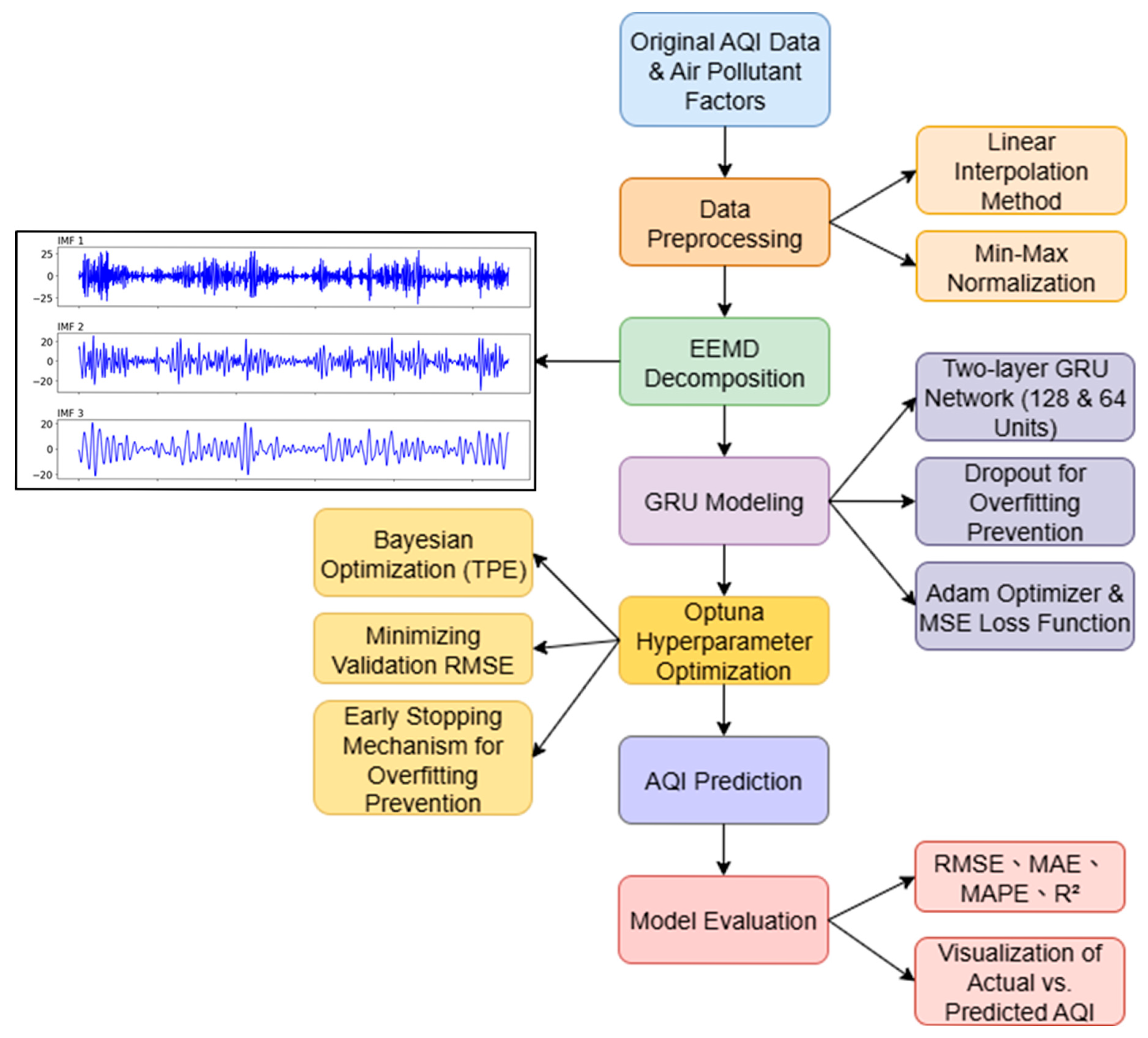
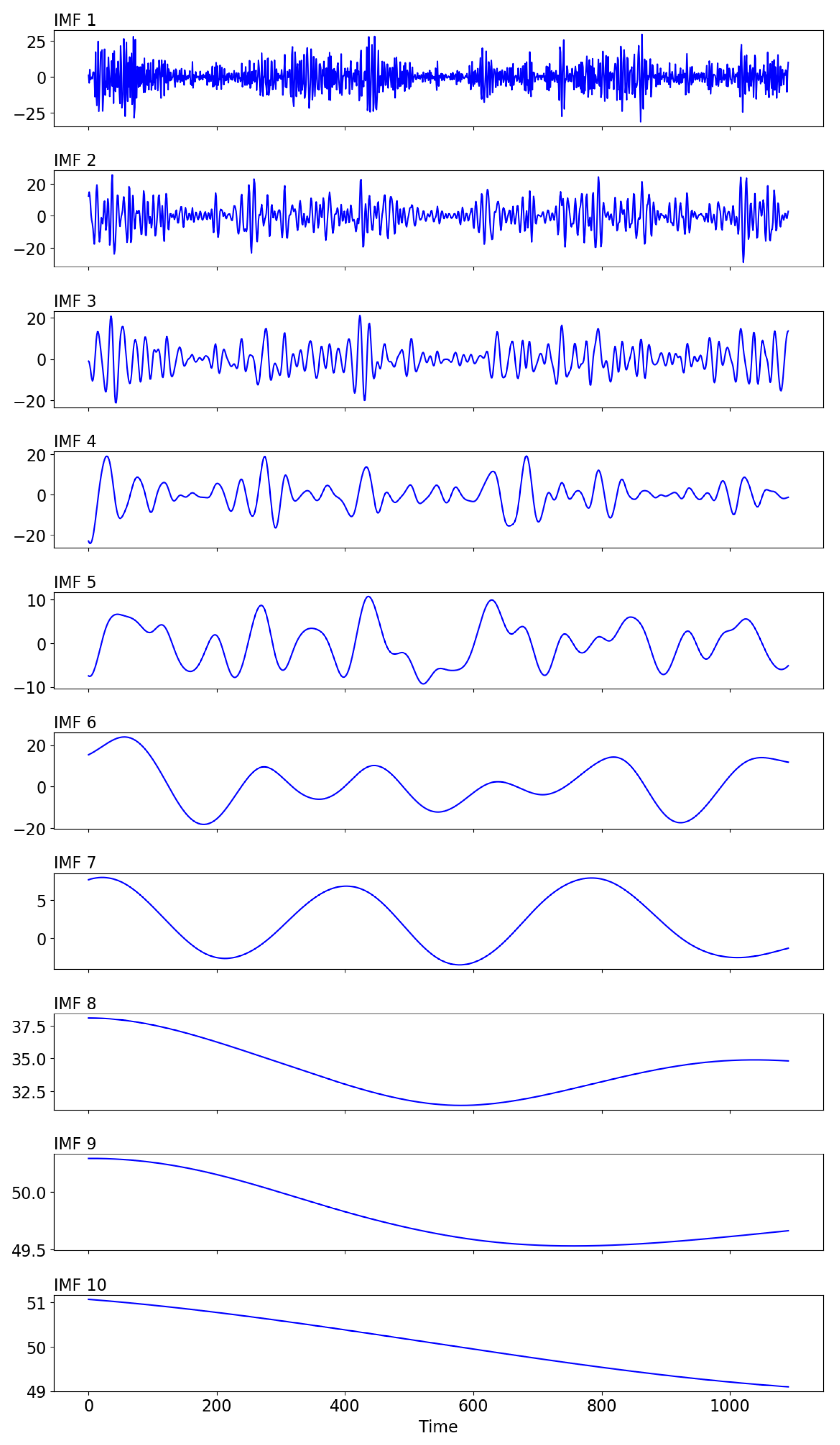
For the AQI time series, EEMD produced 10 IMFs and a residual. Among them, only the first three IMFs were selected as model inputs because they carry the main signal energy and effectively capture short- and mid-term variations. The later IMFs primarily reflect long-term slow trends or random noise, which contribute little to prediction accuracy and may increase model complexity or overfitting risk. This selection therefore preserves essential information, improves stability, and enhances computational efficiency. Figure 2 illustrates the decomposition of AQI into 10 IMFs. The procedure includes:

• Noise addition: Gaussian white noise ${ϵ}_i\left(t\right)$ is added to the original signal $x\left(t\right)$:

  $$x_i\left(t\right)\mathrm{ }=\mathrm{ }x\left(t\right)+{ϵ}_i\left(t\right)$$

  (20)
• EMD on noisy signals: Each perturbed signal undergoes EMD to produce IMFs and a residual:

  $$x_i\left(t\right)\mathrm{ }=\mathrm{ }\sum {IMF}_{i,j}+r_i\left(t\right)$$

  (21)
• Repetition: The noise addition and EMD process is repeated N times for statistical reliability.
• Intrinsic mode function averaging: Corresponding IMFs across all iterations are averaged to obtain a stable and representative set:

  $${IMF}_j\mathrm{ }=\mathrm{ }{\displaystyle \frac{1}{N}}{\sum }_{i=\mathrm{ }1}^N{IMF}_{i,j}$$

  (22)
• Final decomposition: The reconstructed signal is expressed as:

  $$\mathrm{x}\left(t\right)\mathrm{ }=\mathrm{ }\sum {IMF}_j+r\left(t\right)$$

  (23)

This multiscale decomposition allows deep learning models to better capture AQI’s nonlinear and non-stationary behavior.

3.2.5. Hyperparameter Optimization with Optuna

In deep learning, model performance is highly dependent on hyperparameter choices such as the number of layers, units, learning rate, and batch size. To improve predictive accuracy and stability, this study employed Optuna, an automated hyperparameter optimization framework, instead of conventional manual tuning or grid/random search [38]. Optuna applies Bayesian optimization with a Tree-structured Parzen Estimator (TPE), which dynamically adjusts the search strategy based on previous trial results. For the EEMD-GRU model, the search space was defined as follows:

• First-layer GRU units: 32–256
• Second-layer GRU units: 32–128
• Dropout rates: 0.1–0.5
• Learning rate: 1 × 10⁻⁵ to 1 × 10⁻² (log scale)
• Batch size: 16, 32, 64

The objective function minimized the validation RMSE. A total of 20 trials were conducted, and the best-performing configuration was selected for the final model. The chosen parameters were then applied to retrain the EEMD-GRU model using the full training set. To prevent overfitting, an EarlyStopping strategy monitored validation loss and stopped training when no further improvement was observed.

3.3. Proposed Hybrid EEMD-GRU Forecasting Framework

To improve AQI prediction accuracy, this study introduces a hybrid model combining EEMD with GRU neural network, as depicted in Figure 3. The framework integrates multi-scale decomposition, temporal deep learning, and robust performance evaluation:

• Data preprocessing: Daily air quality and meteorological variables were collected, including AMB_TEMP, CH₄, CO, NMHC, NO, NO₂, NO_x, O₃, PM₁₀, PM_2.5, RAINFALL, RH, SO₂, THC, WD_HR, WIND_DIREC, WIND_SPEED, and WS_HR. AQI served as the target variable. Missing values were interpolated using the linear method, followed by Min-Max normalization. This means that each model input consisted of AQI and environmental data from the previous 7 days to predict the AQI for the following day.
• Ensemble empirical mode decomposition: The AQI time series was decomposed into 10 IMFs using EEMD with 100 iterations. Out of theses, the first three IMFs were selected to capture the dominant patterns, as they contain the main signal energy related to short- and mid-term AQI variations. Zero-padding was applied when fewer than three IMFs were generated, ensuring consistent input dimensions.
• Gated recurrent unit architecture: A two-layer GRU network (128 and 64 units) was employed using tanh and sigmoid activations. Dropout (0.2) prevented overfitting. The model was trained with Adam optimizer and MSE loss, with 20% of the data used for test.
• Hyperparameter optimization with Optuna: To identify the best architecture and training configuration, we integrated the Optuna framework, which applies Bayesian optimization (TPE sampler) to minimize validation RMSE. The search space included:
  • first-layer GRU units (32–256),
  • second-layer GRU units (32–128),
  • dropout rates (0.1–0.5),
• learning rate (1 × 10⁻⁵ to 1 × 10⁻², log sampling), and
  • batch size (16, 32, 64).

A total of 20 trials were conducted, with the best configuration applied to the final model. Early stopping monitored validation loss to prevent overfitting.

• Air quality index forecasting: Model outputs were inverse-transformed to their original AQI scale. For multi-step forecasting, a recursive approach was used, feeding predictions back as future inputs.
• Model evaluation: Forecast performance was measured using RMSE, MAE, MAPE, and R², with results visualized through prediction plots and training curves.

To benchmark the effectiveness of the proposed EEMD-GRU model, a comparative framework was developed, integrating various model combinations including LSTM, GRU, and signal decomposition techniques (EMD and EEMD). As shown in Figure 4, this framework provides a comprehensive evaluation of how different model architectures and signal decomposition methods impact AQI forecasting performance, offering insights into optimal configurations for real-world environmental monitoring systems.

3.4. Model Evaluation

To assess forecasting performance, four standard metrics are employed: RMSE, MAE, MAPE, and R². Together, these metrics provide a comprehensive evaluation by capturing absolute, relative, and variance-based prediction errors.

• Root mean squared error (RMSE) quantifies the square root of the average squared differences between predicted and actual values, emphasizing larger deviations and making it sensitive to outliers:

  $$\mathrm{R}\mathrm{M}\mathrm{S}\mathrm{E}\mathrm{ }=\mathrm{ }\sqrt{{\displaystyle \frac{1}{n}}{\sum }_{i=\mathrm{ }1}^n{\left(y_i-{\widehat{y}}_i\right)}^2}$$

  (24)

  where $y_i$ denotes the actual value, ${\widehat{y}}_i$ the predicted value, and n the total number of observations.
• Mean absolute error (MAE) measures the average absolute difference between predictions and observations, offering a straightforward and interpretable assessment of error magnitude. The MAE is defined as:

  $$\mathrm{ }\mathrm{M}\mathrm{A}\mathrm{E}\mathrm{ }=\mathrm{ }{\displaystyle \frac{1}{n}}{\sum }_{i=\mathrm{ }1}^n\left|y_i-{\widehat{y}}_i\right|$$

  (25)
• Mean absolute percentage error (MAPE) expresses errors as a percentage of actual values, facilitating comparisons across datasets with different scales. The MAPE is calculated as:

  $$\mathrm{ }\mathrm{M}\mathrm{A}\mathrm{P}\mathrm{E}\mathrm{ }=\mathrm{ }{\displaystyle \frac{1}{n}}{\sum }_{i=\mathrm{ }1}^n\left|{\displaystyle \frac{y_i-{\widehat{y}}_i}{y_i}}\right|\times 100\%$$

  (26)
• Coefficient of determination (R²)evaluates the proportion of variance in the observed data explained by the model:

  $$R^2=1-{\displaystyle \frac{{\sum }_{i=1}^n{\left(y_i-{\widehat{y}}_i\right)}^2}{{\sum }_{i=1}^n{\left(y_i-\overline{y}\right)}^2}}$$

  (27)

  where $\overline{y}$ is the mean of the observed values.

This combination of evaluation metrics enables a comprehensive and robust comparison of model performance, supporting the identification of the most effective forecasting architecture for AQI prediction.

4. Implementation and Result

4.1. Gray Relational Analysis Results

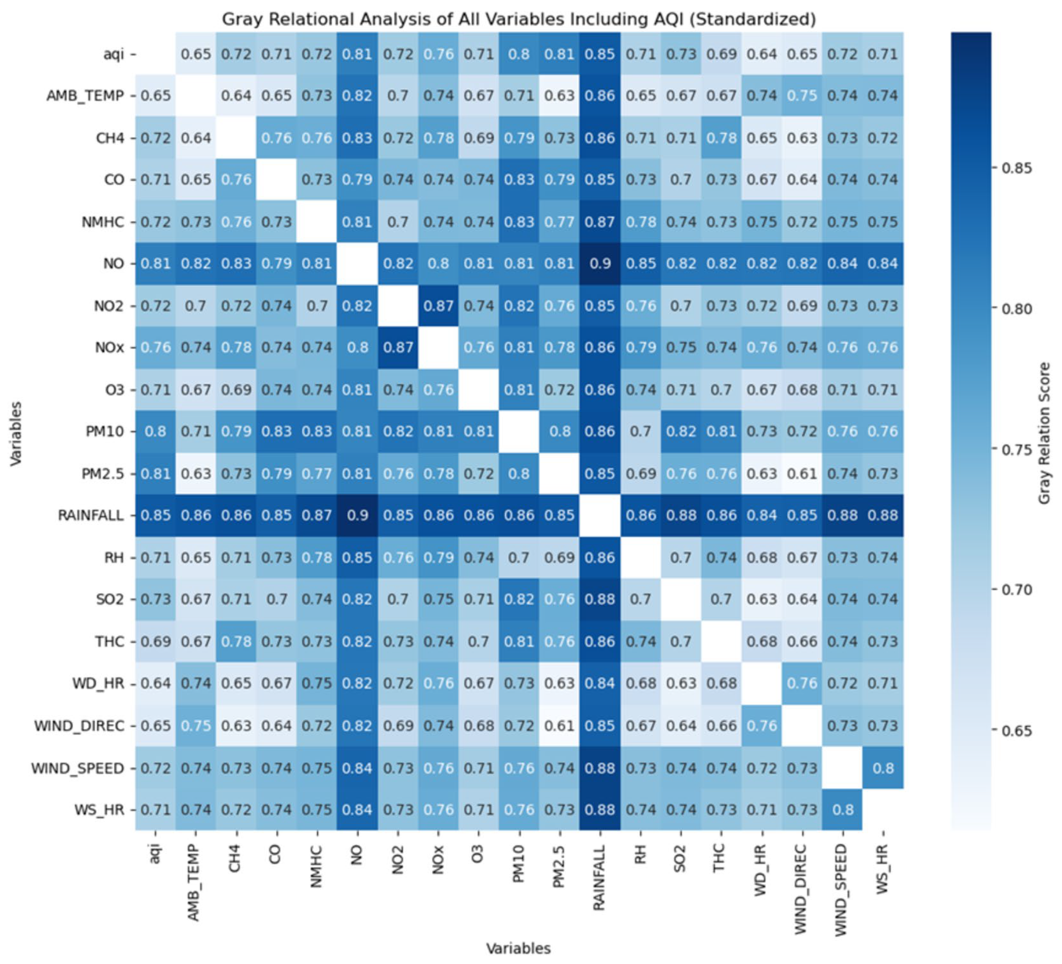
Gray Relational Analysis (GRA) was conducted to evaluate the strength of association between the air quality index (AQI) and various meteorological and pollutant variables. All variables were standardized prior to analysis to ensure comparability. Gray relational coefficients were then computed, where higher values indicate stronger influence on AQI variation. As summarized in

Table 3. Variable ranking by gray relational analysis (GRA).

Rank	Variable	Gray Relational Coefficient
1	RAINFALL	0.85
2	NO	0.81
3	PM2.5	0.81
4	PM10	0.80
5	NOx	0.76
6	SO2	0.73
7	NMHC	0.72
8	NO2	0.72
9	WIND_SPEED	0.72
10	CH4	0.72
11	WS_HR	0.71
12	O3	0.71
13	RH	0.71
14	CO	0.71
15	THC	0.69
16	WIND_DIREC	0.65
17	AMB_TEMP	0.65
18	WD_HR	0.64

, RAINFALL showed the highest correlation with AQI (0.85), followed by NO (0.81) and PM_2.5 (0.81). These results align with existing literature on urban air quality, highlighting the role of precipitation and combustion-related pollutants. In contrast, variables such as AMB_TEMP (0.65) and WD_HR (0.64) exhibited weaker correlations. The complete relational matrix is visualized in Figure 5. Despite variation in individual contributions, all 18 variables were retained in model development to account for potential interaction effects and to ensure generalizability under diverse environmental conditions.

4.2. Model Comparison

4.2.1. Evaluation Metrics and Results

To evaluate forecasting performance, four commonly used metrics were employed: RMSE, MAE, MAPE, and R², capturing both error magnitude and explanatory power. As shown in

Table 4. Model performance comparison.

Model	RMSE	MAE	MAPE (%)	R2
LSTM	10.90	8.33	47.44	0.70
GRU	10.76	7.99	47.46	0.71
EMD-LSTM	8.26	6.29	49.57	0.83
EMD-GRU	7.82	5.87	48.26	0.85
EEMD-LSTM	5.76	4.36	47.93	0.92
EEMD-GRU	5.36	3.96	8.41	0.93
Optuna-EEMD-LSTM	5.62	4.15	9.20	0.92
Optuna-EEMD-GRU	5.12	3.90	8.80	0.93

and Figure S1, the baseline LSTM and GRU models yielded RMSE values of 10.90 and 10.76, respectively. With EMD, these reduced to 8.26 (LSTM) and 7.82 (GRU), and further decreased with ensemble EMD (EEMD) to 5.76 (LSTM) and 5.36 (GRU). MAE followed a similar trend: from 8.33 and 7.99 in baseline LSTM and GRU to 6.29 and 5.87 with EMD, and further to 4.36 and 3.96 with EEMD. Notably, MAPE showed the greatest improvement, declining from 47.46% (baseline GRU) to 8.41% with EEMD-GRU (For supporting data, including actual vs. predicted AQI comparisons using the EEMD-GRU model, see Table S3). This sharp reduction reflects the model’s stronger ability to capture AQI fluctuations once high-frequency noise was separated through decomposition. Since MAPE is highly sensitive when AQI values are low, relative errors on cleaner days tended to be exaggerated in the baseline models. By smoothing the input signal through EEMD, these extreme relative errors were reduced, leading to the substantial improvement observed.

Coefficient of determination values also improved significantly. LSTM rose from 0.70 (baseline) to 0.83 (EMD) and 0.92 (EEMD), while GRU increased from 0.71 to 0.85 (EMD) and 0.93 (EEMD). These results confirm that EMD and EEMD significantly boost model performance by capturing nonlinear and non-stationary AQI patterns. Among all configurations, the EEMD-GRU model consistently outperformed others, making it a promising candidate for real-world AQI forecasting applications.

In addition to classification accuracy, we evaluated the effect of applying PCA for dimensionality reduction. As shown in

Table 5. Forecasting results of the Optuna-EEMD-GRU model with and without PCA.

Model	Cumulative Variance Threshold	R2
Optuna-EEMD-GRU (without PCA)	-	0.94
PCA-Optuna-EEMD-GRU	0.80	0.69
PCA-Optuna-EEMD-GRU	0.90	0.69
PCA-Optuna-EEMD-GRU	0.95	0.71

, PCA with cumulative variance thresholds of 0.80, 0.90, and 0.95 yielded R² values of 0.69, 0.69, and 0.71, respectively. All of these were notably lower than the baseline EEMD-GRU model without PCA (R² = 0.94). These results confirm that PCA did not improve forecasting performance in this study, supporting the decision to retain all 18 input variables.

4.2.2. Statistical Significance Analysis

To further validate the reliability of the results presented in

Table 6. Descriptive statistics of model performance (mean ± std) across five runs.

Model	RMSE	MAE	MAPE	R2
ARIMA	19.484 ± 0.254 A	14.241 ± 0.273 A	28.381 ± 0.431 A	0.197 ± 0.011 A
Prophet	18.879 ± 0.008 B	14.189 ± 0.034 A	31.466 ± 0.181 B	0.103 ± 0.001 A
LSTM	11.354 ± 0.307 C	8.507 ± 0.188 B	18.063 ± 0.309 C	0.675 ± 0.016 A,B
GRU	10.855 ± 0.097 D	8.191 ± 0.106 C	18.286 ± 0.775 C	0.703 ± 0.005 B
EMD-LSTM	8.197 ± 0.143 E	6.406 ± 0.096 D	14.528 ± 0.187 D	0.830 ± 0.005 C
EMD-GRU	8.310 ± 0.153 E	6.498 ± 0.101 D	14.826 ± 0.293 D	0.826 ± 0.006 C
EEMD-LSTM	6.126 ± 0.193 F	4.526 ± 0.140 E	10.363 ± 0.440 E	0.905 ± 0.005 D
EEMD-GRU	5.684 ± 0.053 G	4.187 ± 0.044 F	9.401 ± 0.189 F	0.919 ± 0.001 E
Optuna-EEMD-LSTM	5.543 ± 0.107 G,H	4.141 ± 0.066 F	9.368 ± 0.255 F	0.922 ± 0.003 F
Optuna-EEMD-GRU	5.311 ± 5.311 H	4.014 ± 0.095 F	8.860 ± 0.232 F	0.929 ± 0.003 G
p-value	<0.001	<0.001	<0.001	<0.001

Different superscript letters (A–H) within a column indicate significant differences between models. Models sharing a letter are not significantly different.

, we performed statistical tests to compare the performance of all ten models (ARIMA, Prophet, LSTM, GRU, EMD-LSTM, EMD-GRU, EEMD-LSTM, EEMD-GRU, Optuna-EEMD-LSTM, and Optuna-EEMD-GRU). Each model was trained and evaluated five times, and the mean and standard deviation (mean ± std) of their predictive metrics are reported in Table 6. Overall, integrating empirical mode decomposition (EMD/EEMD) with deep learning architectures substantially improved prediction accuracy and reduced errors.

Among the baseline networks, GRU consistently outperformed LSTM (RMSE = 10.855 vs. 11.354), suggesting that GRU is better suited for handling nonlinear and temporal dependencies in this dataset. When EMD was applied, the error decreased further, with EMD-GRU slightly surpassing EMD-LSTM. Introducing EEMD yielded additional gains, and EEMD-GRU (RMSE = 5.684, R² = 0.919) achieved the best results among models not tuned by Optuna.

Hyperparameter optimization with Optuna further enhanced performance. The Optuna-EEMD-GRU model achieved the lowest RMSE (5.311), the lowest MAPE (8.860%), and the highest R² (0.929), demonstrating superior predictive capability. In addition, the standard deviation across repeated runs decreased as models became more advanced (for example, the standard deviation of R² dropped from 0.016 in LSTM to 0.003 in Optuna-EEMD-GRU), indicating that the improvements were not only in accuracy but also in stability and consistency.

To statistically confirm these observations, a one-way ANOVA was conducted on RMSE, MAE, MAPE, and R² values across all models. The results, summarized in

Table 7. ANOVA results for model performance indicators.

Indicator	F Value	p Value
RMSE	1093.66	3.21 × 10−36
MAE	1091.01	3.33 × 10−36
R2	867.60	1.28 × 10−34
MAPE	429.87	8.79 × 10−30

, show F-values above 400 and p-values much smaller than 0.05 for every metric, clearly indicating significant differences among models.

All p-values were far below the 0.05 threshold, confirming that the observed improvements were statistically significant. This analysis demonstrates that EEMD-based models, particularly Optuna-EEMD-GRU, achieved significantly better performance than traditional time series models and baseline deep learning approaches.

4.2.3. Prediction Graphs

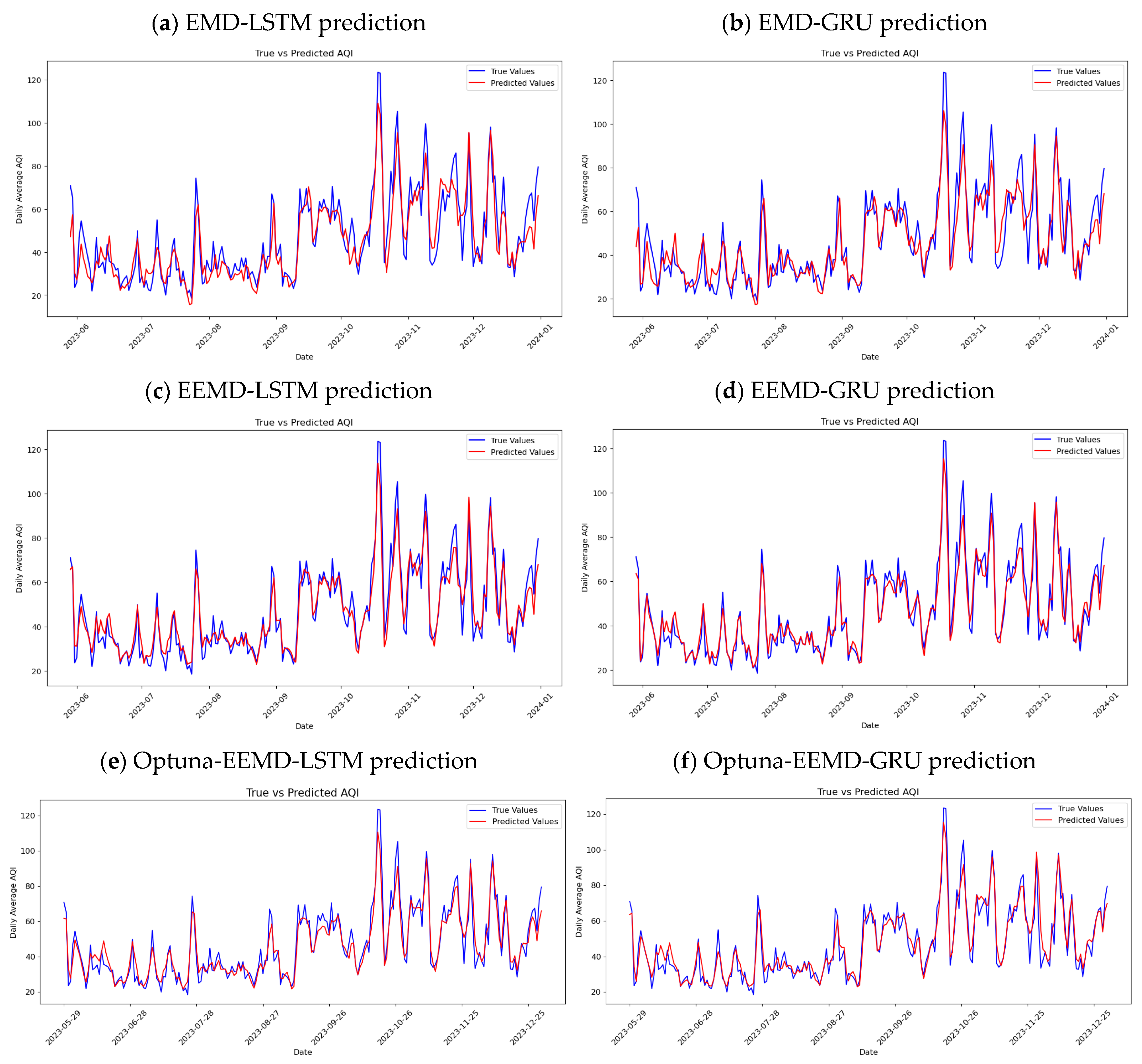
Figure S2 presents visual comparisons between actual and predicted AQI values for the baseline LSTM and GRU models. Both models capture overall trends and directional changes but show noticeable deviations during sharp fluctuations and peak periods. Figure 6 illustrates the prediction results after applying EMD and EEMD. With EMD integration, both EMD-LSTM and EMD-GRU exhibit improved alignment with observed values, especially in capturing temporal dynamics and amplitude variations. These enhancements highlight the benefit of decomposing the original AQI signal into more structured intrinsic mode components before modeling. Further improvements are observed with EEMD. The EEMD-LSTM and EEMD-GRU models closely follow the actual AQI trajectory, particularly in reproducing peaks and troughs. This suggests that EEMD effectively mitigates nonlinearity and nonstationarity in the time series, enabling both GRU and LSTM architectures to extract more relevant features for prediction. Overall, incorporating signal decomposition significantly improves model accuracy. By enhancing feature extraction, EMD and EEMD increase the capacity of deep learning models to handle complex environmental time series. These improvements are essential for real-time air quality forecasting, contributing to more effective public health responses and environmental management strategies.

4.2.4. Training Loss Graphs

Figure S3 and Figure 7. Training and validation loss curves for four model configurations: EMD-LSTM, EMD-GRU, EEMD-LSTM, and EEMD-GRU. display the training and validation loss curves across all model configurations. For the baseline LSTM and GRU models (Figure S3), the loss steadily decreases across epochs, indicating effective model learning. Both training and testing losses follow similar trends, with no signs of overfitting, as shown by the narrow gap between the two curves. In Figure 6, the addition of EMD leads to smoother convergence and reduced loss values in both LSTM and GRU models. The improvement is more pronounced with EEMD, where EEMD-LSTM and EEMD-GRU exhibit the lowest final loss and the tightest alignment between training and validation curves. These results confirm that signal decomposition not only improves predictive accuracy but also enhances model training efficiency and stability. This contributes to better generalization, which is crucial for reliable AQI forecasting in real-world environmental applications.

4.2.5. Prediction Performance of the Optuna-EEMD-GRU Model

Based on the forecasts generated by the Optuna-EEMD-GRU model, predictive accuracy was evaluated using Taiwan’s official air quality standards. Out of 217 testing days, the model correctly predicted the AQI category on 207 days, with only 10 misclassified cases. This corresponds to an overall accuracy of 95.39%, indicating strong reliability of the proposed framework for daily AQI forecasting.

Table 8. Misclassified days in the Optuna-EEMD-GRU model predictions.

Date	Actual Value	Actual Category	Predicted Value	Predicted Category
2023/06/03	54.46	Moderate	47.86	Good
2023/07/08	54.96	Moderate	46.60	Good
2023/09/20	51.25	Moderate	47.79	Good
2023/10/06	55.71	Moderate	48.81	Good
2023/10/27	105.33	Unhealthy for Sensitive Groups	91.92	Moderate
2023/10/29	60.04	Moderate	50.13	Good
2023/12/07	46.83	Good	55.08	Moderate
2023/12/12	56.08	Moderate	49.76	Good
2023/12/22	47.38	Good	51.24	Moderate
2023/12/29	54.54	Moderate	49.75	Good

lists the specific days where misclassification occurred. Most errors involved values close to category thresholds, such as cases where actual AQI was just above or below the boundary between “Good” and “Moderate.” Only one case (27 October 2023) resulted in underestimation of an “Unhealthy for Sensitive Groups” event, while the remaining errors were minor category shifts.

4.3. Model Validation Using Delhi Dataset

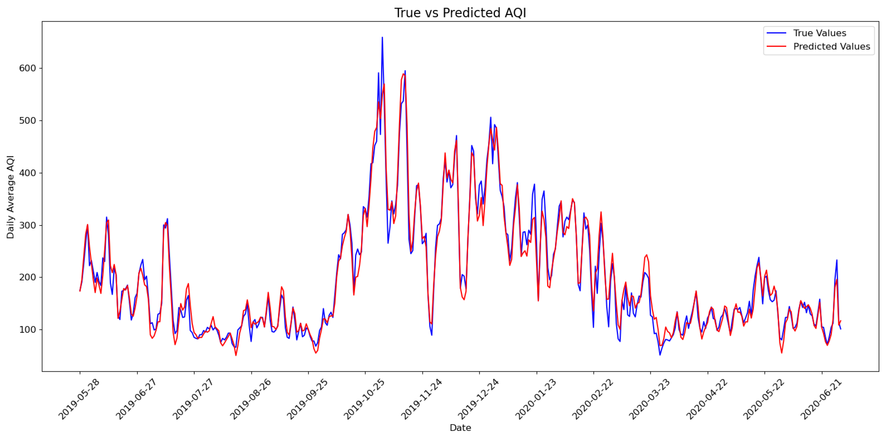
To evaluate the generalizability of the proposed Optuna-EEMD-GRU model, an independent dataset from Delhi, India was used for validation. Figure 8 presents the comparison between actual and predicted AQI values over the testing period. The model demonstrates high fidelity in tracking AQI trends, accurately capturing both short-term fluctuations and long-term patterns. The accompanying training and validation loss curves in Figure 9 exhibit smooth convergence and minimal overfitting, confirming model robustness and stability across training epochs. To benchmark performance against existing literature,

Table 9. Comparison with related studies from Delhi, India.

Author(s) (Year)	Time Period	Model	Variables	R2
This study	Jan 2015–Jul 2020	EEMD-GRU	PM2.5, PM10, NO, NO2, NOx, NH3, CO, SO2, O3, Benzene, Toluene	0.96
Sarkar et al. [28]	Mar 2015–Dec 2021	LSTM-GRU	CO, NO, NO2, NOx, SO2, O3, PM2.5, Temperature, WS, RH, SR	0.84
Gupta et al. [39]	Jan 2015–Jul 2020	CatBoost Regression	PM2.5, PM10, NO, NO2, NOx, NH3, CO, SO2, O3, Benzene, Toluene	0.93
Pande et al. [40]	Jan 2014–Dec 2022	Bi-RNN	PM10, PM2.5, NO, NO2, NOx, O3, CO	0.95

compares the EEMD-GRU model with other AQI forecasting models applied to Delhi, including LSTM-GRU [28], CatBoost Regression [39], and bidirectional recurrent neural network (Bi-RNN) [40]. The proposed model achieved the highest R² value of 0.96, demonstrating superior predictive performance. It should be noted that the Taiwan dataset covers 2021–2023, whereas the Delhi dataset spans 2015–2020. The Delhi data were included to test cross-regional generalizability and to benchmark against existing studies, rather than for direct temporal comparison. Although the time ranges differ, the results still demonstrate the robustness of the model across diverse regions.

5. Conclusions and Future Scope

This study focused on forecasting the air quality index (AQI) by comparing the predictive performance of deep learning models, specifically long short-term memory (LSTM) and gated recurrent unit (GRU) architectures. Both models were implemented with and without integrated data decomposition techniques, including empirical mode decomposition (EMD) and ensemble empirical mode decomposition (EEMD). To ensure the robustness of model training under real-world conditions, comprehensive preprocessing—such as normalization, standardization, and interpolation of missing values—was applied.

Following model development, performance was assessed using multiple evaluation metrics: root mean squared error (RMSE), mean absolute error (MAE), mean absolute percentage error (MAPE), and the coefficient of determination (R²). Training loss curves were also examined to understand convergence behavior. Among the tested configurations, the GRU model integrated with EEMD (EEMD-GRU) demonstrated the best overall performance. The EEMD technique effectively decomposed the AQI time series into smoother components, which facilitated improved feature learning and reduced noise interference. Moreover, the GRU model exhibited greater computational efficiency than LSTM because of its simplified structure and fewer parameters, while still maintaining competitive accuracy. This study contributes to the field in three key ways. First, it introduces a hybrid EEMD-GRU framework that significantly enhances predictive performance by improving input quality and learning stability. Second, the study incorporates 18 environmental and pollutant-related variables—far more than those considered in most prior studies—providing a more comprehensive understanding of AQI determinants and improving the model’s generalizability. Third, the proposed approach offers practical value for environmental monitoring and policy-making. It can serve as a real-time forecasting tool for governmental agencies and environmental institutions to track air quality trends and develop more targeted air pollution control strategies.

Despite these strengths, the study has certain limitations. While the model was validated using data from Xitun District (Taichung, Taiwan) and Delhi (India), its applicability to other geographic regions remains to be tested. Future research should validate the model across a wider range of urban settings to assess its generalizability. Moreover, while EEMD significantly improved performance, exploring alternative decomposition methods such as variational mode decomposition (VMD) or complete ensemble empirical mode decomposition with adaptive noise (CEEMDAN) could yield further enhancements. Investigating the synergistic effects of different preprocessing techniques may also lead to improved forecasting stability and broader application in environmental informatics.

References

1. Chen, J.; Dahlin, M.J.; Luuppala, L.; Bickford, D.; Boljka, L.; Burns, V.; Johnson, M.S. Air pollution and climate change: Sustainability, restoration, and ethical implications. In Air Pollution Sources, Statistics and Health Effects; Nova Science Publishers: New York, NY, USA, 2021; pp. 279–325. [Google Scholar]
2. Sivarethinamohan, R.; Sujatha, S.; Priya, S.; Sankaran; Gafoor, A.; Rahman, Z. Impact of air pollution in health and socio-economic aspects: Review on future approach. Mater. Today Proc. 2021, 37, 2725–2729. [Google Scholar] [CrossRef]
3. Kampa, M.; Castanas, E. Human health effects of air pollution. Environ. Pollut. 2008, 151, 362–367. [Google Scholar] [CrossRef]
4. Almetwally, A.A.; Bin-Jumah, M.; Allam, A.A. Ambient air pollution and its influence on human health and welfare: An overview. Environ. Sci. Pollut. Res. 2020, 27, 24815–24830. [Google Scholar] [CrossRef]
5. WHO. WHO Global Air Quality Guidelines: Particulate Matter (PM2.5 and PM10), Ozone, Nitrogen Dioxide, Sulfur Dioxide and Carbon Monoxide; World Health Organization: Geneva, Switzerland, 2021. [Google Scholar]
6. Sillmann, J.; Aunan, K.; Emberson, L.; Büker, P.; Van Oort, B.; O’Neill, C.; Otero, N.; Pandey, D.; Brisebois, A. Combined impacts of climate and air pollution on human health and agricultural productivity. Environ. Res. Lett. 2021, 16, 093004. [Google Scholar] [CrossRef]
7. Spezzano, P. Mapping the susceptibility of UNESCO world cultural heritage sites in Europe to ambient (outdoor) air pollution. Sci. Total Environ. 2021, 754, 142345. [Google Scholar] [CrossRef]
8. Oliveira, M.L.; Neckel, A.; Pinto, D.; Maculan, L.S.; Zanchett, M.R.D.; Silva, L.F. Air pollutants and their degradation of a historic building in the largest metropolitan area in Latin America. Chemosphere 2021, 277, 130286. [Google Scholar] [CrossRef]
9. Zhang, M.; Liu, X.; Ding, Y. Assessing the influence of urban transportation infrastructure construction on haze pollution in China: A case study of Beijing-Tianjin-Hebei region. Environ. Impact Assess. Rev. 2021, 87, 106547. [Google Scholar] [CrossRef]
10. Wu, C.-H.; Tsai, I.-C.; Tsai, P.-C.; Tung, Y.-S. Large-scale seasonal control of air quality in Taiwan. Atmos. Environ. 2019, 214, 116868. [Google Scholar] [CrossRef]
11. Wong, Y.J.; Shiu, H.-Y.; Chang, J.H.-H.; Ooi, M.C.G.; Li, H.-H.; Homma, R.; Shimizu, Y.; Chiueh, P.-T.; Maneechot, L.; Sulaiman, N.M.N. Spatiotemporal impact of COVID-19 on Taiwan air quality in the absence of a lockdown: Influence of urban public transportation use and meteorological conditions. J. Clean. Prod. 2022, 365, 132893. [Google Scholar] [CrossRef] [PubMed]
12. Kao, C.-L.; Fang, G.-C.; Gao, W.-S.; Zhuang, Y.-J. Concentrations, size distributions, and seasonal variations of ambient air pollutants (particulates, trace metals) in Daya/Xitun District, Taichung, Central Taiwan: A case study at Taichung Science Park. J. Environ. Sci. Health Part A 2021, 56, 824–834. [Google Scholar] [CrossRef] [PubMed]
13. Das, R.; Middya, A.I.; Roy, S. High granular and short-term time series forecasting of PM2.5 air pollutant: A comparative review. Artif. Intell. Rev. 2022, 55, 1253–1287. [Google Scholar] [CrossRef]
14. Al-Mukhtar, M. Random forest, support vector machine, and neural networks to modelling suspended sediment in Tigris river-Baghdad. Environ. Monit. Assess. 2019, 191, 673. [Google Scholar] [CrossRef]
15. Del Ser, J.; Casillas-Perez, D.; Cornejo-Bueno, L.; Prieto-Godino, L.; Sanz-Justo, J.; Casanova-Mateo, C.; Salcedo-Sanz, S. Randomization-based machine learning in renewable energy prediction problems: Critical literature review, new results and perspectives. Appl. Soft Comput. 2022, 118, 108526. [Google Scholar] [CrossRef]
16. Hochreiter, S.; Schmidhuber, J. Long short-term memory. Neural Comput. 1997, 9, 1735–1780. [Google Scholar] [CrossRef]
17. Chung, J.; Gulcehre, C.; Cho, K.; Bengio, Y. Empirical evaluation of gated recurrent neural networks on sequence modeling. arXiv 2014, arXiv:1412.3555. [Google Scholar] [CrossRef]
18. Jiang, T.; Liu, Y. A short-term wind power prediction approach based on ensemble empirical mode decomposition and improved long short-term memory. Comput. Electr. Eng. 2023, 110, 108830. [Google Scholar] [CrossRef]
19. Wu, Q.; Lin, H. A novel optimal-hybrid model for daily air quality index prediction considering air pollutant factors. Sci. Total Environ. 2019, 683, 808–821. [Google Scholar] [CrossRef] [PubMed]
20. Beig, G.; Ghude, S.D.; Deshpande, A. Scientific Evaluation of Air Quality Standards and Defining Air Quality Index for India. Citeseer 2010. Available online: http://www.tropmet.res.in/~lip/Publication/RR-pdf/RR-127.pdf (accessed on 4 July 2025).
21. Imam, M.; Adam, S.; Dev, S.; Nesa, N. Air quality monitoring using statistical learning models for sustainable environment. Intell. Syst. Appl. 2024, 22, 200333. [Google Scholar] [CrossRef]
22. Zhu, S.; Lian, X.; Liu, H.; Hu, J.; Wang, Y.; Che, J. Daily air quality index forecasting with hybrid models: A case in China. Environ. Pollut. 2017, 231, 1232–1244. [Google Scholar] [CrossRef] [PubMed]
23. MOENV. Taiwan Air Quality Monitoring Network. Available online: https://airtw.moenv.gov.tw/ENG/default.aspx (accessed on 4 July 2025).
24. Wang, J.; Li, H.; Lu, H. Application of a novel early warning system based on fuzzy time series in urban air quality forecasting in China. Appl. Soft Comput. 2018, 71, 783–799. [Google Scholar] [CrossRef]
25. Janarthanan, R.; Partheeban, P.; Somasundaram, K.; Elamparithi, P.N. A deep learning approach for prediction of air quality index in a metropolitan city. Sustain. Cities Soc. 2021, 67, 102720. [Google Scholar] [CrossRef]
26. Du, S.; Li, T.; Yang, Y.; Horng, S.-J. Deep air quality forecasting using hybrid deep learning framework. IEEE Trans. Knowl. Data Eng. 2019, 33, 2412–2424. [Google Scholar] [CrossRef]
27. Espinosa, R.; Palma, J.; Jiménez, F.; Kamińska, J.; Sciavicco, G.; Lucena-Sánchez, E. A time series forecasting-based multi-criteria methodology for air quality prediction. Appl. Soft Comput. 2021, 113, 107850. [Google Scholar] [CrossRef]
28. Sarkar, N.; Gupta, R.; Keserwani, P.K.; Govil, M.C. Air quality index prediction using an effective hybrid deep learning model. Environ. Pollut. 2022, 315, 120404. [Google Scholar] [CrossRef]
29. Shewalkar, A. Performance evaluation of deep neural networks applied to speech recognition: RNN, LSTM and GRU. J. Artif. Intell. Soft Comput. Res. 2019, 9, 47–54. [Google Scholar] [CrossRef]
30. Gao, S.; Huang, Y.; Zhang, S.; Han, J.; Wang, G.; Zhang, M.; Lin, Q. Short-term runoff prediction with GRU and LSTM networks without requiring time step optimization during sample generation. J. Hydrol. 2020, 589, 125188. [Google Scholar] [CrossRef]
31. Yang, S.; Yu, X.; Zhou, Y. LSTM and GRU neural network performance comparison study: Taking Yelp review dataset as an example. In Proceedings of the 2020 International Workshop on Electronic Communication and Artificial Intelligence (IWECAI), Tianjin, China, 12–14 June 2020; IEEE: Piscataway, NJ, USA, 2020; pp. 98–101. [Google Scholar] [CrossRef]
32. Gao, Y.; Wang, R.; Zhou, E. Stock prediction based on optimized LSTM and GRU models. Sci. Program. 2021, 2021, 4055281. [Google Scholar] [CrossRef]
33. Agarwal, N.; Meena, C.S.; Raj, B.P.; Saini, L.; Kumar, A.; Gopalakrishnan, N.; Kumar, A.; Balam, N.B.; Alam, T.; Kapoor, N.R. Indoor air quality improvement in COVID-19 pandemic. Sustain. Cities Soc. 2021, 70, 102942. [Google Scholar] [CrossRef]
34. CTSP. Central Taiwan Science Park. 2025. Available online: https://www.ctsp.gov.tw/english/00home/home.aspx?v=20. (accessed on 4 July 2025).
35. Gers, F.A.; Schmidhuber, J.; Cummins, F. Learning to forget: Continual prediction with LSTM. Neural Comput. 2000, 12, 2451–2471. [Google Scholar] [CrossRef]
36. Selvin, S.; Vinayakumar, R.; Gopalakrishnan, E.; Menon, V.K.; Soman, K. Stock price prediction using LSTM, RNN and CNN-sliding window model. In Proceedings of the 2017 International Conference on Advances in Computing, Communications and Informatics (ICACCI), Udupi, India, 13–16 September 2017; IEEE: Piscataway, NJ, USA, 2017; pp. 1643–1647. [Google Scholar] [CrossRef]
37. Puttagunta, M.; Ravi, S. Medical image analysis based on deep learning approach. Multimed. Tools Appl. 2021, 80, 24365–24398. [Google Scholar] [CrossRef]
38. Akiba, T.; Sano, S.; Yanase, T.; Ohta, T.; Koyama, M. Optuna: A next-generation hyperparameter optimization framework. In Proceedings of the 25th ACM SIGKDD International Conference on Knowledge Discovery & Data Mining (KDD ’19), Anchorage, AK, USA, 4–8 August 2019; ACM: New York, NY, USA, 2019; pp. 2623–2631. [Google Scholar] [CrossRef]
39. Gupta, N.S.; Mohta, Y.; Heda, K.; Armaan, R.; Valarmathi, B.; Arulkumaran, G. Prediction of air quality index using machine learning techniques: A comparative analysis. J. Environ. Public Health 2023, 2023, 4916267. [Google Scholar] [CrossRef]
40. Pande, C.B.; Kushwaha, N.L.; Alawi, O.A.; Sammen, S.S.; Sidek, L.M.; Yaseen, Z.M.; Pal, S.C.; Katipoğlu, O.M. Daily scale air quality index forecasting using bidirectional recurrent neural networks: Case study of Delhi, India. Environ. Pollut. 2024, 351, 124040. [Google Scholar] [CrossRef] [PubMed]
Figure 1. Original AQI data used for model training and evaluation.
Atmosphere 16 01095 g001
Figure 2. AQI time series decomposed into 10 intrinsic mode functions (IMFs) and a residual using EEMD.
Atmosphere 16 01095 g002
Figure 3. Optuna-EEMD-GRU Model.
Atmosphere 16 01095 g003
Figure 4. Comparative model framework.
Atmosphere 16 01095 g004
Figure 5. Gray correlation analysis diagram.
Atmosphere 16 01095 g005
Figure 6. Prediction graphs of AQI values using EMD-LSTM, EMD-GRU, EEMD-LSTM, EEMD-GRU, and Optuna-EEMD-GRU models.
Atmosphere 16 01095 g006
Figure 7. Training and validation loss curves for four model configurations: EMD-LSTM, EMD-GRU, EEMD-LSTM, and EEMD-GRU.
Atmosphere 16 01095 g007
Figure 8. AQI prediction results of Delhi, India using the Optuna-EEMD-GRU model.
Atmosphere 16 01095 g008
Figure 9. Training and validation loss of the Optuna-EEMD-GRU model for AQI prediction in Delhi, India.
Atmosphere 16 01095 g009