Abstract
To explore the spatiotemporal evolution of extreme temperature events in Guangxi (1940–2023), reveal regional response mechanisms, and assess future trends of persistence under climate warming, a multi-scale analysis was conducted using ERA5 reanalysis data. Methodologies included RH tests for homogeneity correction, collaborative kriging for data optimisation, Mann–Kendall tests for trend and abrupt change detection, Morlet wavelet analysis for cyclic pattern identification, Exploratory Spatio-Temporal Data Analysis (ESTDA) for spatial heterogeneity quantification, and Rescaled Range (R/S) analysis to calculate Hurst indices for future persistence assessment. Results showed the following: (1) The ERA5 dataset exhibited high applicability in Guangxi (R = 0.9989, RMSE = 1.9492 °C), supporting robust evidence of continuous warming—warm indices (e.g., SU25, TX90p) increased significantly (SU25 at 0.2044 d/10a), while cold indices (e.g., TN10p, FD0) declined (TN10p at −0.0519 d/10a); abrupt changes of cold indices were concentrated in 1942–1950, with warm indices accelerating post-2000 and TXx exhibited the highest warming rate (0.23 °C/decade). (2) Extreme temperature indices displayed a primary 19–21-year oscillation cycle (dominant in warm indices) and a secondary 13-year cycle (prominent in cold indices). (3) Spatial heterogeneity featured northwest–southeast cold–heat inversion, coastal–inland intensity gradients, and latitudinal zonation of extreme indices; ESTDA revealed intensified polarisation, with warm indices clustering in low-latitude regions (e.g., Baise) and cold indices declining homogeneously in mountainous areas (e.g., Guilin), indicating an irreversible transition to a warming steady state. (4) R/S analysis indicated all indices had Hurst indices of 0.65–0.92, reflecting persistent future trends consistent with historical evolution, with warm indices (e.g., TNn, SU25) showing stronger persistence (H > 0.85). This work clarifies the spatial polarisation mechanism and future persistence of extreme temperature dynamics in Guangxi, providing a multi-scale scientific basis for disaster early warning and adaptation planning in climate-sensitive karst-monsoon regions.
1. Introduction
In the context of global warming, the frequency and intensity of Extreme Temperature Events (ETEs) have increased and become a frontier area of climate change research. The Sixth Assessment Report of the IPCC indicates that the frequency of extreme high temperature events increased by 2.8 times globally from 1980 to 2020, while the frequency of extreme low temperature events decreased by 34% [1]. Climate system anomalies have posed a multidimensional threat to human society and ecological environment [2]; Wang Huijun, Yuan Yufeng and other researchers showed that the global high temperature threshold in 2023–2024 consecutively exceeded the historical record, and the warming amplitude reached 1.55 °C compared with the pre-industrial revolution, which marks the advent of the “global boiling era”, and the economic losses and the frequency of extreme weather events are exponentially increasing [3,4]. Based on the analysis of 1980–2022 data, Xu Xinyao et al. revealed that 33% of the global land area showed a persistent aridity trend, and the spatial proportion of winter drought area expanded to 33.2%, which was significantly higher than that of humidified area (10%) [5]. Through a CMIP6 multi-model ensemble simulation, Quartz’s team confirmed that the global average temperature will continue to climb in 2021–2100, and the warming is significantly and positively correlated with greenhouse gas emission scenarios [6].
Climate assessment, as a core part of climate change research [1], systematically analyses the long-term evolution of the climate system, the risk of extreme events and their ecological–socio-economic chain effects by integrating observational data, simulation results and impact assessment models, with the core objective of providing scientific support for regional adaptation strategies. Yiting Wang et al. pointed out that global warming, as a major driving factor, causes the frequency and intensity of extreme temperature and precipitation events to reorganise at the global scale by changing the atmospheric circulation and energy balance [7]. This kind of reorganisation shows significant regional polarisation characteristics in the subtropical monsoon zone. Wang et al. showed that Guangxi, as a concentration of karst landscapes in Southwest China, has a unique and typical climate system response to global warming, which urgently needs to be revealed through multi-scale assessment of the intrinsic mechanisms [8].
Important progress has also been made in China’s regional scale studies: Wang Shaowu et al. found that the 1940s–1950s were influenced by the natural climate fluctuations in the Northern Hemisphere and the stable period of the monsoon circulation, the national temperature variability was relatively small, but cold extremes were frequent in the south [9]; Zhou Baiquan et al. pointed out that in the 1980s–1990s, along with the accelerated global warming (rate of 0.2 °C/decade) and weakening of the summer winds of East Asia (about 12 per cent) [10], warm winter phenomena appeared in Guangxi and other places in 1986–1999, which increased 1.3 °C from 1961–1985 in winter mean. The phenomenon of warm winters was revealed in Guangxi and other places, and the average winter temperature in 1986–1999 increased by 1.3 °C compared with that in 1961–1985. The 2022 China Climate Bulletin shows that extreme events since the 21st century have shown the polarisation feature of “warmer and drier”, and the number of high temperature days in 2020 was 20.6% higher than normal [11]. The evolution of the climate cycle further reveals the intrinsic law of China’s climate system. The last two climate cycles (1940–1970 and 1980–2010), which are bounded by solar activity and ENSO quasi-cycles, show significant differences [12]: the first cycle is characterised by cold extremes and moderate precipitation, and the number of frost days in Guangxi reaches more than 20 days per year on average; and the second cycle shifts to warm extremes, which is accompanied by a sharp shift of droughts and floods and an intensification of spatial polarisation [13]. Hu Yichang et al. showed that the number of warm night (cold night) days increased (decreased) at a rate of 10.3 d/10a (−7.8 d/10a), and the rate of change in the number of warm day (cold day) days was 5.9 d/10a (−3.6 d/10a) in the whole country from 1961 to 2020 [14]. The Blue Book on Climate Change in China emphasises that the warming rate in South China (0.16 °C/10a) is significantly higher than the national average, among which Guangxi (0.16 °C/10a warming from 1961–2020), as a typical karst-monsoon climate zone [15], has a special necessity for its extreme temperature study.
At the methodological level, earlier studies were limited in comparability of findings due to heterogeneous definitions of extreme temperature indices and thresholds, especially in quantifying the effects of combined heat and humidity stress [16]. The 27 standardised extreme temperature indices (ETIs) proposed by the World Meteorological Organisation (WMO) ETCCDI have become an international benchmarking system due to their scientific and universal applicability [17,18]. Existing studies in Guangxi have revealed the spatial and temporal variability of ETEs: Chen et al. pointed out that the number of extreme high-temperature days increased at a rate of 4.3 days/decade from 1990 to 2015 [18]; and Huang Lei et al. found that a “thermal corridors (High-temperature zones)” with a warming rate of 1.2 °C was formed along the Hechi-Nanning route from 2010 [19]. Despite the progress made, there are still three limitations in the current study: 1. Data reliability: although the ERA5 reanalysis data are highly reliable in Southwest China [20], the precision of the application in Guangxi region is still doubtful; 2. Insufficient analysis of the mechanism: limited by the static spatial analysis method [21], the dynamic interaction process of the ETEs and the multiscale driving mechanism are still unclear; 3. Insufficient prediction ability: lack of quantitative prediction of future trends and the continuity of future trends. Insufficient prediction ability: lack of quantitative prediction of future trend continuity and deep excavation of historical cyclical patterns.
How to couple high-resolution data with spatio-temporal models to analyse the multi-scale driving mechanisms and thus support climate resilience planning has become a key scientific issue. This study aims to establish a climate assessment framework for karst region and provide theoretical support for regional ecological protection and agricultural adaptation. Based on the ERA5 reanalysis dataset of 111 districts and counties in Guangxi from 1940 to 2023, we cross-checked the applicability of the data by Pearson’s correlation coefficient and root-mean-square error (RMSE) [22], calculated 10 core indices of ETCCDI, and constructed a whole chain analysis framework of “data optimisation-trend diagnosis-periodic analysis-spatial and spatial-temporal deconstruction-future prediction”. We adopt RHtests homogeneity correction to improve data quality, collaborate with Kriging spatial interpolation to generate multi-scale datasets [23], comprehensively use Mann–Kendall trend test [24], Morlet wavelet transform [25] and ESTDA model [26] to systematically reveal the spatial and temporal evolution law of the ETEs and introduce the R/S analytical model to compute the Hurst index [27], and quantitatively predict the ETCCDI core indices [27]. to quantitatively predict the future persistence characteristics of ETEs.
2. Data Sources and Methods
2.1. Overview of the Study Area
Guangxi, located in southwest China, comprises 14 prefecture-level cities and 111 counties (as of October 2023) with a total land area of 237,600 km2 and a jurisdictional sea area of 7000 km2 [28]. It features a typical karst landform on the southeastern edge of the Yunnan-Guizhou Plateau, under a low-latitude subtropical monsoon climate [29]. Extreme temperatures range from −2.0 °C to 42.5 °C, with a multi-year average of 21.4 °C. Summer is dominated by the subtropical high, leading to frequent high temperatures and meteorological droughts—here specifically referring to droughts triggered by persistent high temperatures (e.g., Tmax > 35 °C) coupled with reduced precipitation, aligning with the extreme temperature dynamics analysed. Observational data show Guangxi’s annual mean temperature rose significantly at 0.23 °C/10 years (1981–2020), with consecutive rainless days increasing at 4.1 days/10 years [30]. The 2009–2010 mega drought, a typical case of such temperature-induced meteorological drought, damaged 2.78 million hectares of crops and caused over USD 3.2 billion in direct losses, the most severe agrometeorological disaster in the region since modern meteorological records began [31]. The study area is shown in Figure 1.
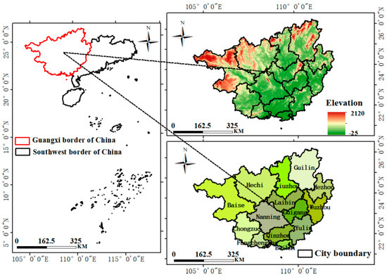
Figure 1.
A brief map of the geographical location of Guangxi Zhuang Autonomous Region.
2.2. Data Sources
In this study, the meteorological data are obtained from the ERA5 dataset of the European Centre for Medium-Range Weather Forecasts “https://www.ecmwf.int/ (accessed on 15 December 2024)”, and the daily maximum and daily minimum temperature data of 111 counties and districts in Guangxi for the years 1940–2023 are selected for the study, with a resolution of 0.25° × 0.25°, and a temporal coverage of a total of 84 years of 1940–2023 years of data data, focusing on its spatial subset in Guangxi Zhuang Autonomous Region, China (104°29′–112°04′ E, 20°54′–26°24′ N), which contains the complete spatial coverage of 14 municipalities. The Guangxi DEM data were obtained from the Geospatial Data Cloud (http://www.gscloud.cn/, accessed on 15 December 2024) with a resolution of 30 m. The station observations used to examine the ERA5 dataset in this study were obtained from ground-based meteorological observation stations under the Nanning Meteorological Bureau (NMB), and the time span of the observation data was from January 1980 to December 2023.
2.3. Research Methodology
2.3.1. Pearson’s Correlation Coefficient and Root Mean Square Error
In order to assess the applicability of the ERA5 reanalysis dataset to temperature data in Guangxi, this study used two statistical indicators, Pearson correlation coefficient and Root Mean Square Error (RMSE), to cross-validate the ERA5 reanalysis dataset in terms of the trend consistency and numerical deviation dimensions [32]. Pearson’s correlation coefficient (R) is used to measure the linear correlation between the ERA May mean temperature data and the ground observation data, and its value ranges from [−1, 1]. The closer it is to 1, the more consistent the trend is, and it is calculated as follows:
In this formula, and are the average temperature values of ERA5 data and observed data in the i-th month, respectively, and are the mean values of ERA5 data and observed data, respectively, and n is the sample size.
Root mean square error (RMSE) is used to quantify the degree of numerical deviation of ERA5 data from the observed data, the unit is consistent with the air temperature (°C), the smaller the RMSE value, indicating that the absolute error of the ERA5 data is smaller, the higher the numerical accuracy of the calculation formula is:
The combination of the two methods can comprehensively evaluate the applicability: a high R value (close to 1) indicates that ERA5 can accurately capture the temporal and spatial variation trend of temperature in Guangxi, while a low RMSE value (<2 °C) indicates that its numerical simulation accuracy meets the research requirements. The two values together constitute the reliability of ERA5 data set in temperature analysis in Guangxi.
2.3.2. Extreme Temperature Index
The International Panel on Climate Diagnostics and Indices (ETCCDI) proposed a set of 27 indices calculated from daily temperature and daily precipitation data, which are widely used in the international arena, and are characterised by weak extremes, low noise, and high significance [33]. In this paper, the most representative 10 extreme temperature indices are selected to identify the extreme temperature events in Guangxi Region, and the definitions and codes are listed in Table 1. In order to ensure the credibility and reliability of the data in each county, this paper checks the homogeneity of the information and quality control, and uses the RHtests homogeneity correction with spatial interpolation to fill in the gaps. Calculations were performed in RclimDex software 1.1 [34].

Table 1.
Definition of extreme temperature index.
2.3.3. Analysis of Sudden Changes in Extreme Temperatures and Spatial Analysis
Trends in the evolution of extreme climate indices were identified as statistically significant by the Mann–Kendall (M-K) non-parametric test, and the magnitude of the quantitative trend was estimated using the Theil-Sen (T-S) slope [35]. Climate mutation points were verified by the M-K ordinal statistic mutation test, with the intersection of the UF-UB curves and exceeding the confidence interval (p < 0.05) as the criterion for determination. Spatial analysis based on the Kriging interpolation method to generate the spatial distribution of climate indices in Guangxi.
2.3.4. Extreme Temperature Cycle Analysis
Morlet wavelet analysis is a time–frequency analysis method based on complex-valued wavelet function, and its core advantage lies in the ability to capture the time domain and frequency domain information of the time series at the same time, and decompose the original data into the superposition of different frequency components through wavelet transform, which in turn reveals the characteristics of the data’s local changes in the time and frequency dimensions [17]. In the study of extreme temperatures, Morlet wavelet analysis can effectively detect the cyclic changes of extreme temperature indices, the characteristics of abrupt changes and their evolution over time [25]. The dimensionless frequency of Morlet wavelet is set to 6 to balance the time-frequency resolution, and the oscillatory cycles of extreme temperatures can be identified by the modal values of wavelet coefficients.
2.3.5. Extreme Temperature Exploratory Spatio-Temporal Data Analysis (ESTDA)
ESTDA provides a multidimensional perspective for analysing complex geographic phenomena by integrating information in the temporal and spatial dimensions [36]. Firstly, the global Moran’s I index is used to measure the spatial autocorrelation characteristics of the whole region and identify the spatial clustering degree of extreme temperature events; secondly, the local Moran’s I index and its scatterplot are used to reveal the spatial distribution characteristics of the four local spatial correlation patterns, namely, the high-value clusters (high–high), the low-value clusters (low–low) and the anomalies (high–low, low–high), and investigate the local spatial correlation patterns based on the exploration of temporal and spatial data. The spatial distribution characteristics of the four types of local spatial correlation patterns of high value clusters (high–high), low value clusters (low–low) and anomalies (high–low, low–high) are revealed, and the spatial and temporal patterns of extreme temperature indices in Guangxi are systematically analysed based on the framework of Exploratory Spatio-Temporal Data Analysis (ESTDA).
In order to further characterise the spatio-temporal dynamics, the study introduces the LISA time path and LISA spatio-temporal jump method, which characterises the evolutionary strength and trend of spatial correlation patterns through the parameters of relative length, curvature and direction angle [37]. When the relative length is larger than 1, it indicates more dynamic local spatial dependence and local spatial structure, and the smaller it is, the more stable it is. When the curvature is greater than 1, it indicates that the study area is more influenced by the neighbouring space, and the smaller it is, the weaker the influence of the neighbouring space is.
where N is the relative length; D is the curvature; T is the time interval; Li, t is the position of city i in Moran’s I scatterplot in year t; d(Li,t, Li,s+1) is the distance moved by city i at moments t~t + 1.
At the same time, the LISA spatio-temporal jump model is constructed, and the regional state is divided into four types of spatio-temporal transfer types based on the Markov chain theory as shown in Table 2, and the dynamic stability of spatial pattern is quantified by calculating the spatio-temporal jump probability (SC) and spatio-temporal cohesion (SF), so as to reveal the intrinsic law of the spatio-temporal evolution of the extreme temperatures.
where SSF and SSC are the spatio-temporal flow coefficient and spatio-temporal cohesion coefficient, respectively, MA, MB, MC, and MD are the number of leaps of types A, B, C, and D, respectively, and m is the total number of leaps.
Table 2.
Basic types of time-space teleportation.
2.3.6. Re-Scaled Extreme Variance Analysis (R/S)
Hurst index based on R/S analysis is an effective method to quantitatively characterise the long-term dependence of time series information, which is especially suitable for revealing the nonlinear dynamics in complex systems [38]. The method determines the persistence or anti-persistence characteristics of a time series by standardising the polar deviation and standard deviation of the time series. The core steps include: splitting the time series into multiple equal-length sub-series, calculating the cumulative deviation polar deviation (R) and standard deviation (S) of each sub-series separately, and solving the Hurst index (H) based on the logarithmic regression of the R/S ratio of different sub-series lengths. When H = 0.5, the sequence is stochastic; 0 < H < 0.5 shows anti-persistence and the current trend may be reversed; 0.5 < H < 1 shows persistence and the current trend will continue to evolve. In this study, this method is used to quantitatively analyse the persistence characteristics of the trends of 10 extreme temperature indices in Guangxi.
2.3.7. Methodological Frameworks and Software
The methodological flow used in this study is shown in Figure 2. Data preprocessing was done in Python 3.1.1 environment, including sequence homogeneity test based on RHtests algorithm, missing value interpolation filling and ERA5 dataset adaptation calculation; extreme value index calculation and trend diagnosis were done in R 4.2.1 platform using RClimDex package to generate the ETCCDI standard indices, and Mann–Kendall test was performed, Morlet wavelet analysis and R/S persistence assessment; spatial pattern construction relies on the Geostatistical Analyst module of ArcGIS 10.0 and interpolates county statistics to a 1 km resolution using ordinary kriging and a spherical semivariational model (block = 0.2, partial block = 1.3, range = 18 km) and a 15-point neighbourhood search; spatial and temporal evolution indices calculation and trend diagnosis are performed on the R 4.2.1 platform using the RClimDex software package. The resolution of the spatial and temporal evolution was performed by GeoDa 1.20, a module that calculates the global Moran I index and the LISA time path parameters (relative length, curvature, direction of movement). Finally, all spatial results (index distribution maps, LISA clustering maps and spatio-temporal path evolution maps) were visualised and integrated in ArcGIS 10.8.
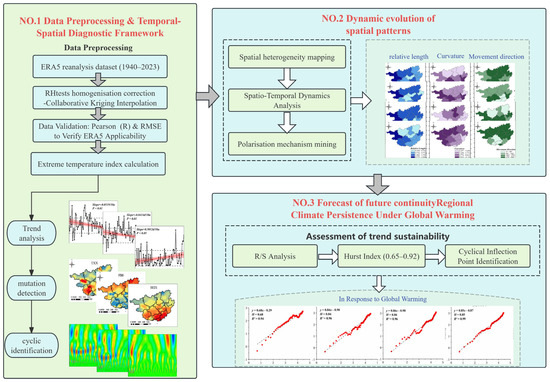
Figure 2.
The methodology flowchart.
3. Results and Analysis
3.1. ERA5 Reanalysis Dataset Adaptation Analysis
Due to the lack of measured station data for the period 1940–1979, this study used a segmented cross-validation method to assess the reliability of the ERA5 data for that time period. The correlation coefficient reaches 0.9989 (nearly 1), indicating that ERA5’s monthly mean temperature data show nearly perfect consistency with observed trends, accurately capturing seasonal fluctuations and long-term variations in Guangxi’s climate. This result significantly exceeds the “high applicability” threshold (R ≥ 0.85) [32] in meteorological data validation, demonstrating its reliability in temperature trend simulation. The root mean square error (RMSE) stands at 1.9492 °C, within acceptable meteorological error ranges. Decadal analysis reveals stable RMSE values between 1.86–2.02 °C, showing no significant fluctuations. Notably, after 2000, RMSE slightly decreased to 1.86–1.96 °C (as shown in Figure 3). Both trend consistency (R ≈ 0.999) and numerical accuracy (RMSE ≈ 1.95 °C) meet ideal standards, satisfying requirements for climate analysis and trend studies.
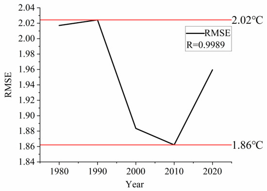
Figure 3.
shows the decade-by-decade variation of RMSE between ERA5 data and observation data from 1980 to 2023 (Unit: °C).
3.2. Characteristics of Temporal and Spatial Changes of Extreme Temperature Index in the Recent 80a
3.2.1. Characteristics of Extreme Temperature Index Changes in the Last 80a
As shown in Figure 4, TX90p, TN90p, SU25, and WSDI show significant upward trends in the warmth index of the Guangxi the period 1940–2023. Among them, SU25 shows the most obvious upward trend, while TX90p shows the relatively slowest increase. As for the cold index, FD0, TX10p, TN10p, and CSDI all show significant decreasing trends. Among them, TN10p showed the fastest rate of decrease, while FD0 showed the slowest rate of decrease. The extreme value indices TXx and TNn showed an increasing trend, with TXx showing the fastest rate of increase and TNn the slower rate of increase.
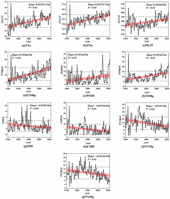
Figure 4.
Trend of extreme temperature index in Guangxi from 1940 to 2023.
The M-K mutation test shows that the mutation of extreme temperature indices started in 1942, and the indices with the most concentrated mutation occurred during 1942–1950, and the evolution of extreme temperatures has a phase characteristic: the mutation of cold indices (CSDI, FD0, etc.) was concentrated in 1942–1950,Warm index mutation in 1950–2019 (accelerated after 2000), and the extreme indices of TXx, and TNn undergo significant jumps in 2002–2013 and 2015–2019, respectively. Combined with the time-series analysis, it is shown that the frequency of cold events decreases sharply from the 1980s onwards, and the warm events surge after 2000, and the polar indices, such as TXx, are the most sensitive to the warming response. Multi-method cross-validation reveals that the Guangxi climate system has experienced a three-stage evolution of cold event decay (1940s), warm event accumulation (2000s), and extreme heating value intensification (2010s) in the last 84 years, with an overall significant warming trend.
Due to the limitation of space, only some indices are shown in this paper, and the results are shown in Figure 5. As can be seen from Table 3, the first major cycle of most extreme temperature indices is concentrated in 19–21 years, and the peaks of wavelet variance in this interval are significant and the oscillations are violent. The main indices involved are TX90p, TN90p, SU25, TXX, TNN and WSDI, among which, TX10p, FD0 and TN10p indices show obvious oscillation patterns [see Figure 5a,b,d], with the first major period of about 13 years, and all of them have three obvious oscillations, and the first major period of TX90p and TN90p is 21 years. TX90p and TN90p both have a first principal cycle of 21 years, but TX90p has three more distinct oscillatory cycles [see Figure 5c], while TN90p has only two distinct oscillatory cycles.
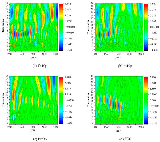
Figure 5.
Real part of wavelet contour lines of extreme temperature index (a–d) in Guangxi.
Table 3.
Analysis results of extreme temperature index trend and cycle.
3.2.2. Characteristics of the Spatial Distribution of the Extreme Temperature Index
The spatial distribution of the extreme temperature index is shown in Figure 6. Among the warm indices, the spatial distribution of TX90p and TN90p is also consistent, with the low-value area mainly distributed in the southeast corner of Guangxi, covering Yulin City, Guigang City and Wuzhou City, etc.; the high-value area is concentrated in the western part of Baise City; the high-value area of the SU25 index is mainly distributed in Beihai City and Yulin City, and the low-value area is in Baise City; the high-value area of the WSDI index is concentrated in Wuzhou City in the eastern part of Guangxi, while the low-value area is in Baise City in the west and in the north, showing a decreasing characteristic from east to west. The low value areas are in Baise in the west and Guilin in the north, showing a decreasing characteristic from east to west. Among the cold indices, TX10p and TN10p show similar spatial distribution characteristics, with their high values concentrated in the southwestern part of Baise and low values located in the northwestern corner of Baise; the extremes of the FD0 index are concentrated in the Guilin area, and low values are located in the central-south region of Guangxi, including Laibin and Nanning, etc., and the high values of the CSDI index are concentrated in part of Liuzhou, and the low values are distributed in the Hechi, Guilin, etc., with no distribution, and Guilin, etc., with no obvious single recurrence pattern in distribution. Among the extreme value indices, the TNn index shows a stepwise increasing distribution from low to high values from north to south, with the low-value area concentrated in Guilin City and the high-value area located in Beihai City; the high-value area of the TXx index is more dispersed, mainly located in Baise City, Laibin City, and the central part of Chongzuo City, while the low-value area is located in Guilin City.
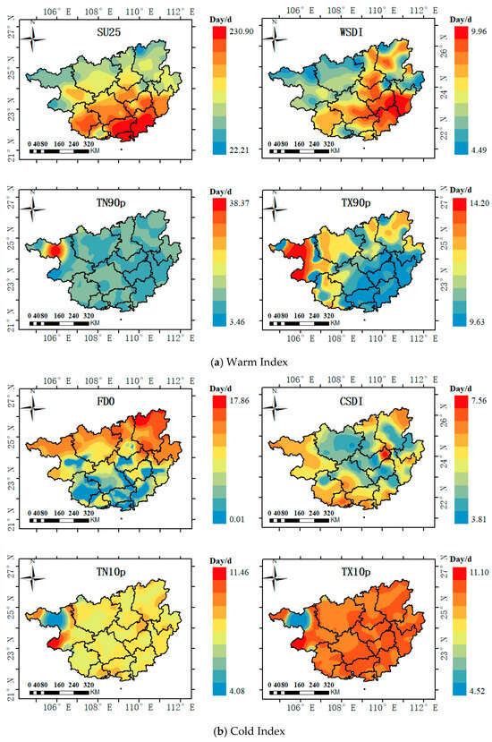
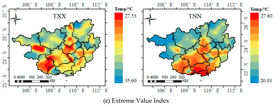
Figure 6.
Spatial distribution of extreme climate index (a–c) in Guangxi.
3.3. Exploratory Spatio-Temporal Data Analysis (ESTDA)
3.3.1. LISA Time Path
Spatial visualisation of the geometric features of the LISA time paths for the Guangxi extreme temperature index was carried out in arcgis 10.8 software, with relative lengths, curvatures and movement methods classified into four categories according to the natural breakpoint method. Based on the comprehensive analysis of Figure 7 (Due to space limitations, only the indices of six are listed the spatial differentiation characteristics of extreme climate indices in Guangxi show significant regional differences.
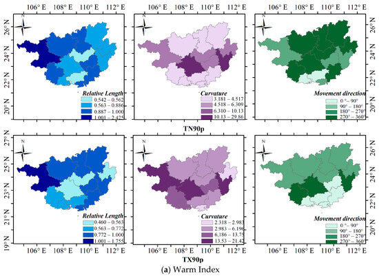
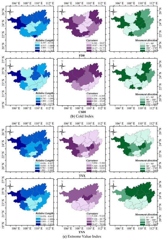
Figure 7.
Spatial distribution of LISA time path spatial characteristics of extreme climate index (a–c) in Guangxi.
The spatial distribution characteristics of the curvature parameter further corroborate the variability of the regional extreme temperature indices (in Figure 7). The curvature values of all the extreme temperature indices are >1, indicating that the cities are strongly influenced by their neighbours, among which the WSDI and SU25 indices show moderate curvature in central Guangxi, with mean values of 0.45 ± 0.11 and 0.48 ± 0.13, respectively, which show a relatively stable trend of change. fd0, TN10p, and TNN show the lowest curvature, with mean values of 0.28 ± 0.07, 0.31 ± 0.08, and 0.29 ± 0.06, which may be related to the regional variability of extreme temperature indexes (in Figure 7). 0.07, 0.31 ± 0.08, and 0.29 ± 0.06, which may be related to the decrease in the frequency of cold events in the context of regional warming. The curvature of the CSDI and TN90 indices are 0.33 ± 0.09 and 0.38 ± 0.10, respectively, whose lower spatial fluctuation characteristics may be related to the homogenising effect of warming. Txx, Tx10p, and Tx90phave curvatures of 0.36 ± 0.10, 0.42 ± 0.12 and 0.40 ± 0.11, respectively, reflecting moderate spatial and temporal fluctuations.
The analysis of spatial movement direction reveals the trend of spatial agglomeration of climate events (Figure 7, right). The movement direction of WSDI index in central Guangxi mainly points to “high–high agglomeration”, with a quadrant average movement direction angle of 332° ± 16°, and the movement direction of SU25 index also shows the same trend, with an average movement direction angle of 328° ± 14°. fd0 index moves towards “low–low agglomeration”, with a quadrant average movement direction angle of 142° ± 12°. The fd0 index moves in the direction of “low–low agglomeration” with an average quadrant angle of 142° ± 12°, while the TN10p and TNN indices show a similar trend, with average angles of 138° ± 15° and 145° ± 13°, respectively. the CSDI index moves in the direction of “low–low agglomeration” with an average angle of 145° ± 13°. The CSDI index moves in a predominantly “low–low concentration” direction, with an average angle of 135° ± 10°, while the TN90p shows a trend towards “high–high concentration”, with an average angle of 318° ± 13°. The Txx, Tx10p, and Tx90p all show a similar trend, with an average angle of 138° ± 15° and 145° ± 13°, respectively. Txx, Tx10p and Tx90p all move in the direction of “high–high agglomeration” with an average angle of movement of 325° ± 15°, 335° ± 18° and 322° ± 16°, respectively.
3.3.2. LISA Space-Time Migration (Spatial Markov Chain)
Through the coordinates of the Moran’s I scatter plot of the extreme temperature index in Guangxi, the different types of leap probabilities are calculated for 1940–2020, and then the spatio-temporal leap probability SC and spatio-temporal cohesion SF of each index are obtained. The results are shown in Table 4.
Table 4.
Transfer probability matrix of extreme temperature index Local Moran’s I.
For the extreme value index, there are 8 and 12 Class A leapfrog cities in TXx and TNn, accounting for 57.1% and 85.7%, respectively. Both of them show low cohesion (0.2143 for TXx and 0.1429 for TNn) with high leaping probability (0.7857 for TXx and 0.8571 for TNn), and the spatial reconstruction process of TXx exhibits a continuous leaping pattern in the Guizhong Plain, whereas TNn exhibits jumping abruptness in the mountainous area of northwest Gui.
For the warm index, the spatial dynamics of TX90p (cohesion of 0.4286 and jump probability of 0.5714) is in between the warm and cold events. TX90p and TN90p have the majority of class D jump cities, 8 and 5, respectively, accounting for 57.1% and 35.7%. TN90p has the highest spatial and temporal cohesion (0.5) and the lowest jump probability (0.5), and has the most stable spatial pattern; There are 11 class A leap cities of SU25, accounting for 78.6%, and 8 class D leap cities of WSDI index, accounting for 57.1%. The spatial and temporal parameters of WSDI and CSDI are the same, but the spatial leap vectors of WSDI are oriented to the high value area for aggregation. The cohesion degree of SU25 is slightly higher (0.2143), and the probability of jumping amounts to 0.7857, and the spatial reconstruction of the high temperature sustained event is active.
For the cold index, TX10p and TN10p have the majority of class A leap cities, 9 and 7, respectively, accounting for 64.3% and 50%; TX10p (cohesion of 0.3571, leap probability of 0.6429) and TN10p (cohesion of 0.4286, leap probability of 0.5714) have high leap probabilities, and the spatial distributions of the cold day and cold night events have frequent changes; the FD0 index (0.1429), with the lowest cohesion (0.8571) and the highest jump probability (0.1429), and the spatial distribution is unstable; and the CSDI (0.3571, 0.6429), with the spatial and temporal parameters of cohesion (0.3571) and jump probability (0.6429), which is characterised by multidirectional discretisation, accounted for 7 cities in the CSDI (50 percent) and the D class. In addition, the spatio-temporal cohesion of all indices is significantly negatively correlated with the leap probability, indicating that there is a mutually constraining relationship between stability and variability in the spatial distribution of extreme climate events.
3.4. Analysis of Future Trends
Based on 84 years of extreme temperature data, this study used R/S analysis to assess the trend persistence of extreme temperature in Guangxi. The results show that all indices Hurst indices are significantly greater than 0.5 (0.65–0.92), indicating that the future trend is in the same direction as the historical evolution. The warm indices (TX90p, TN90p, SU25, WSDI) show a significant upward trend, while the cold indices (FD0, TX10p, TN10p, CSDI) significantly decrease. Figure 8 clearly demonstrates the persistent character of the trend of each index through the linear relationship of ln(R/S)-ln(t) double logarithmic coordinate system. It is worth noting that the CSDI index shows a clear inflection point at ln(t) = 1.8 (corresponding to the time scale t ≈ 6a), which marks the existence of an average cyclic fluctuation cycle of about 6a in the number of cold persistence days, and most of the other index cycles are concentrated in 12–16a. The consistency feature of the Hurst index confirms that there is a significant inertial effect of the regional extreme temperature change, and the cycle length of the quantitative results provide a time scale reference for the predictability study of extreme climate events. The extreme temperature index Hurst index and a comparison of past and future trends are shown in Table 5.
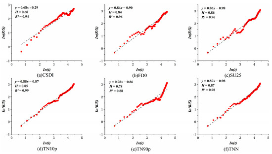
Figure 8.
Trend of Hurst index of extreme climate index in Guangxi.
Table 5.
Comparison of extreme temperature index Hurst index with past and future trends.
4. Discussions
Against the backdrop of intensifying global warming, frequent extreme temperature events have emerged as a critical threat to ecological security [1]. In climate-sensitive karst regions of Southwest China, these events exhibit marked spatial heterogeneity in their response mechanisms [8]. Leveraging ERA5 reanalysis data across 111 Guangxi districts/counties (1940–2023), this study transcends conventional linear climate analyses through multiscale cycle decomposition and ESTDA spatial modelling, systematically revealing nonlinear evolution in regional extreme temperatures. Key findings demonstrate accelerated warming across Guangxi, with warm indices showing growth rates significantly correlated to 19–21-year primary and 13-year secondary climatic oscillations. Spatially, a three-dimensional pattern emerges: northwest–southeast thermal inversion, coastal–inland intensity gradients, and stepwise extreme-value responses. Marginal mountainous areas exhibit heightened warm-index volatility compared to low-elevation zones, while cold indices display spatially homogenised recession—patterns were potentially linked to the weakening of East Asian winter monsoon and Siberian High southward displacement, requiring verification via circulation indices. These conclusions align with urban heat island differentiation in South China [39] and CMIP6 RCP8.5 projections of accelerated Guangxi warming [40], reinforcing result reliability.
Analysis reveals cold-index mutation points (e.g., FD0, TX10p) clustered predominantly in the 1940s–1950s (Table 3), coinciding with documented cold-extreme frequency in southern China. This temporal correspondence reflects large-scale circulation modulation—notably East Asian winter monsoon intensity and Siberian High positioning—of low-temperature events during an era dominated by natural climate variability [9]. Conversely, warm-index abrupt changes (e.g., TX90p, TN90p) occurred post-2000 (2002–2019), aligning temporally with accelerated global warming phases characterised by ~12% East Asian summer monsoon weakening [3,4]. Monsoon attenuation prolonged subtropical high dominance, directly intensifying and spatially expanding warm extremes (e.g., high-temperature days, warm days/nights), thereby explaining observed “thermal corridors (high-temperature zones)” such as the Hechi–Nanning warming axis [19]. Northwest-southeast temperature gradient reversal (Figure 6), particularly warm-index clustering alongside cold-index homogenisation in northwestern karst highlands (e.g., Baise), likely stems from karst-driven surface energy repartitioning (valley inversions, slope effects) coupled with altered cold-air pathways under weakening winter monsoons, reducing southern low-altitude cold exposure [10]. Despite the overall recessionary trend of the cold index, FD0 shows high volatility (SF = 0.1429) in mountainous areas (e.g., Guilin), reflecting the modulation of extreme low temperature events by local topography. Critically, Hurst index analysis confirms persistent future trends (H > 0.68; Table 5), with robust warm-index continuity (H > 0.75) aligning with CMIP6 RCP8.5 projections. This indicates probable continuation of increasing warm-extreme frequency/intensity and declining cold events under current GHG emission trajectories.
Methodologically, this work quantifies spatiotemporal heterogeneity while revealing the “homogenized cold-index decline versus polarized warm-index surge” differentiation pattern, offering novel perspectives for climate science. Practically, results enable dynamic identification of high-risk zones in marginal mountains, guiding precise resource allocation for disaster prevention. Synergising with Guangxi’s “climate-resilient city” goals (Ecological Civilization Construction Plan 2021–2035) and Xijiang River Basin restoration initiatives, intensified warming polarisation in northwestern mountains necessitates prioritising heat-resilient infrastructure in Baise and Hechi within regional climate adaptation frameworks. Furthermore, findings provide theoretical foundations for designing temperature-responsive ecological compensation mechanisms.
Several limitations warrant consideration. First, ERA5 exhibits systematic biases in complex terrain; future work should couple humidity data with thermal stress indices (e.g., UTCI) to quantify humidity-heat synergy effects. Second, urbanisation’s contribution to the Baise “heat corridor” remains unquantified; integrating NPP-VIIRS night-time lights with RegCM experiments could disentangle natural versus anthropogenic warming interactions. Finally, as Hurst indices disregard socioeconomic scenarios, subsequent efforts should integrate multi-source data to develop calibrated mountain-temperature models, employ RegCM nesting to quantify drivers, and fuse Hurst with CMIP6 projections into dual-driver risk assessment frameworks. Such advances would establish a comprehensive “climate-ecology-socioeconomy” risk evaluation system, supporting sustainable karst development.
5. Conclusions
Using the ERA5 reanalysis dataset covering 111 districts and counties in Guangxi from 1940 to 2023, this study systematically analysed the evolution of extreme temperatures by integrating nonlinear trend diagnosis and spatio-temporal dynamic jump theory, verifying the research hypotheses proposed in the introduction. The key findings are as follows:
Data reliability and warming trends: The ERA5 dataset demonstrates high applicability in Guangxi, with a Pearson correlation coefficient (R) of 0.9989 and a root mean square error (RMSE) of 1.9492 °C, confirming its effectiveness in capturing regional temperature dynamics [32,40]. Based on this validated data, Guangxi exhibits a persistent warming trend: warm indices (e.g., SU25, TX90p) show significant increases, while cold indices (e.g., TN10p, FD0) decline, with TN10p decreasing at −0.0519 days per decade. Among extreme value indices, TXx shows the highest warming rate (0.23 °C per decade). Abrupt changes in cold indices are concentrated in 1942–1950, whereas warm indices accelerated after 2000 (2002–2019), reflecting stage-specific differences in regional responses to climate warming.
Cyclic patterns: Extreme temperature indices exhibit distinct periodic characteristics, with a primary oscillation cycle of 19–21 years (dominant in warm indices such as TX90p and TN90p) and a secondary cycle of 13 years (prominent in cold indices such as TX10p and FD0). Most indices show superimposed oscillations of these primary and secondary cycles.
Spatial heterogeneity and polarisation mechanisms: The spatial distribution of extreme temperatures is characterised by three-dimensional heterogeneity: (1) northwest–southeast cold–heat inversion, (2) coastal–inland intensity gradients, and (3) latitudinal zonation of extreme indices. The ESTDA model reveals intensified spatial polarisation: warm indices form high-value clusters in low-latitude regions (e.g., Baise), while cold indices show homogeneous decline in mountainous areas (e.g., Guilin). LISA time path analysis indicates strong neighbour-dependent spatial dynamics (curvature > 1), with warm indices aggregating toward “high-high” clusters and cold indices converging toward “low–low” clusters, marking an irreversible transition of the regional climate system to a warming steady state.
Future persistence and methodological value: R/S analysis indicates all extreme temperature indices have Hurst indices ranging from 0.65 to 0.92 (all > 0.5), reflecting persistent future trends consistent with historical evolution. Warm indices (e.g., TNn, SU25) exhibit strong persistence (H > 0.85), while cold indices (e.g., CSDI) show relatively weak but stable persistence (H = 0.68). The integrated methodological framework—incorporating RHtests homogeneity correction, collaborative kriging interpolation, Mann–Kendall trend tests, Morlet wavelet analysis, ESTDA, and R/S analysis—provides a robust multi-scale tool for quantifying extreme climate dynamics, ensuring the reproducibility and comparability of results [23,26,27].
This study clarifies the spatial polarisation mechanisms and future persistence of extreme temperature responses in Guangxi, offering scientific support for disaster early warning and climate adaptation in karst-monsoon regions. The validated dataset and systematic methodological chain lay a foundation for further related research.
Author Contributions
S.H. wrote the main manuscript text, X.T. responsible for the polishing of the article. All authors have read and agreed to the published version of the manuscript.
Funding
This research was funded by [Research and application of dynamic resource security and ecological environment “trade-off” assessment technology for clean energy industry in Guilin] grant number [20230111-1].
Institutional Review Board Statement
Not applicable.
Informed Consent Statement
Not applicable.
Data Availability Statement
The meteorological data supporting the findings of this study are available in the Copernicus Climate Data Store (CDS) under the accession code [ERA5 hourly data on single levels from 1940 to present, DOI: 10.24381/cds.adbb2d47]. If there is a need to access the data used in this study, please contact the corresponding author Xiangling Tang, Email: txling@glut.edu.cn.
Conflicts of Interest
The authors declare no conflicts of interest.
References
- China Meteorological News. IPCC Sixth Assessment Report Working Group II Report Released; China Meteorological News: Beijing, China, 2022. [Google Scholar]
- Zhou, B.; Qian, J. Interpreting the IPCC AR6 report: Changes in extreme weather and climate events. Prog. Clim. Change Res. 2021, 17, 713–718. [Google Scholar]
- Wang, H.; Sun, J.; Chen, L.; Ma, J.H.; Duan, M.K. Global warming and accelerating climate extremes: A review of major advances in climate research in China in 2024. J. Atmos. Sci. 2025, 48, 1–7. [Google Scholar]
- Yuan, Y.; Liao, Z.; Zhou, B.; Zhai, P. Progress in the study of high-impact regional extreme events and attribution in China under the background of increasing global warming. Prog. Clim. Change Res. 2025, 21, 44–55. [Google Scholar]
- Xu, X.; Wang, X.; Zhang, S.; Yang, Y.; Li, Z. Characteristics of spatial and temporal variations of global land drought and its future trends. Plateau Meteorol. 2025, 44, 1–15. [Google Scholar]
- Shi, Y.; Xu, Y.; Chao, Q.; Zhang, M.; Han, Z.; Wang, R. Future climate change prediction in the western route of south-to-north water transfer project area based on CMIP6 multi-model. Prog. Clim. Change Res. 2025, 21, 1–14. [Google Scholar]
- Wang, Y.; Li, S.; Wu, L.; Cai, W.; Geng, T. Enhanced response of multi-year intergenerational variability to global warming in the Atlantic Ocean. Sci. Bull. 2025, 70, 2616–2618. [Google Scholar] [CrossRef] [PubMed]
- Wang, Y.; Su, Y.; Li, Z. Response of temperature change to global warming in Guangxi from 1961 to 2010. J. Nat. Resour. 2013, 28, 1707–1717. [Google Scholar]
- Wang, S.; Luo, Y.; Zhao, Z.; Wen, X.; Huang, J. Paleoclimate modelling. Prog. Clim. Change Res. 2013, 9, 305–308. [Google Scholar]
- Zhou, B.; Yang, T.; Zhou, B.; Sun, J.; Wang, Q.; Zhai, P. Progress of regional climate change prediction in China. J. Meteorol. 2025, 83, 716–728. [Google Scholar]
- China Meteorological Administration. China Climate Bulletin 2022; Meteorological Publishing House: Beijing, China, 2023.
- Roy, I.; Haigh, J.D. Solar cycle signals in sea level pressure and sea surface temperature. J. Geophys. Res. 2010, 115, 116. [Google Scholar] [CrossRef]
- Chen, L.; Zhou, X.; Li, W.; Lu, Y.; Zhu, W. Characteristics of climate change in China over the past 80 years and its formation mechanism. J. Meteorol. 2004, 5, 634–646. [Google Scholar]
- Hu, Y. A study of extreme temperature trends in China considering data homogeneity and autocorrelation. Meteorol. Sci. Technol. 2025, 53, 211–221. [Google Scholar]
- China Meteorological Administration Climate Change Center (CMACC). China Blue Book on Climate Change. Energy Conserv. Environ. Prot. 2024, 7, 1. [Google Scholar]
- Yin, H.; Sun, Y. Characterisation of extreme temperature and precipitation in China based on the ETCCDI index in 2017. Adv. Clim. Change Res. 2019, 15, 363–373. [Google Scholar]
- Chu, X.; Wu, W.; Yang, X.; Wang, H. Extreme climate change and future trend prediction in the Tumen River Basin over the past 60 a. Water Resour. Hydropower Technol. 2024, 55, 24–37. (In English) [Google Scholar]
- Chen, X.; Li, H.; Huang, W. Characteristics of spatial and temporal variations of extreme heat events in South China and analysis of influencing factors. Prog. Clim. Change Res. 2018, 14, 445–456. [Google Scholar]
- Qin, W.; Li, Y. Analysis of the causes of meteorological disasters of high temperature and heat wave in Guangxi in 2010. Meteorol. Res. Appl. 2011, 32, 13–16. [Google Scholar]
- Zhang, W.; Zhou, T.; Zhang, L. Evaluation of air temperature from ERA5 reanalysis over the Tibetan Plateau and its surrounding regions. J. Geophys. Res. Atmos. 2021, 126, e2020JD033786. [Google Scholar]
- Liu, Y.; Chen, H.; Wang, S. Spatiotemporal Analysis of Extreme Temperature Events over China: A Review. Int. J. Climatol. 2020, 40, 1429–1445. [Google Scholar]
- Liu, T.; Zhu, X.; Zhang, S.; Xu, K.; Guo, R. Applicability of ERA5 reanalysis of surface air temperature data in China. J. Trop. Meteorol. 2023, 39, 78–88. [Google Scholar]
- Jang, D.; Kim, N.; Choo, H. Kriging Interpolation for Constructing Database of the Atmospheric Refractivity in Korea. Remote Sens. 2024, 16, 2379. [Google Scholar] [CrossRef]
- Wang, R.; Cao, Y. Characterisation of climate change analysis of tourism in Ili River Valley—Based on Mann-Kendall test. Knowl. Econ. 2024, 3, 9–12. [Google Scholar]
- Xu, X.; Yu, S.; Liu, Z.; Su, L.; Gao, F. Temporal and spatial distribution characteristics of extreme temperature index in the ecological demonstration area and surrounding areas of Northwest Sichuan. Plateau Meteorol. 2025, 1–15. [Google Scholar] [CrossRef]
- Hao, S.; Sun, C.; Song, Q. Evaluation of water ecological footprint and water ecological stress in China based on ESTDA model. J. Ecol. 2021, 41, 4651–4662. [Google Scholar]
- Liu, X.; Xiao, L.; Gao, G.; Cheng, Y.; Li, L. Characteristics of spatial and temporal evolution of extreme temperature index and its influencing factors in Guizhou Province from 1960 to 2020. Water Resour. Hydropower Technol. 2025, 56, 39–50, (In English and Chinese). [Google Scholar]
- Guangxi Zhuang Autonomous Region Bureau of Statistics. Guangxi Statistical Yearbook 2023; China Statistics Press: Beijing, China, 2023; pp. 4–5.
- Luo, S.; He, W.; Yang, T.; Deng, Y.; Lv, Y.; Wu, K.; Meng, Q. Geological significance and formation mechanism of geomorphological development features in the Xianggui Corridor. China Karst 2021, 40, 750–759. [Google Scholar]
- Guangxi Zhuang Autonomous Region Climate Centre. Guangxi Climate Change Monitoring Report (1961–2020); Guangxi Zhuang Autonomous Region Climate Centre: Nanning, China, 2024; pp. 56–61. [Google Scholar]
- Department of Water Resources of Guangxi Zhuang Autonomous Region. Guangxi Flood and Drought Disaster Defence Bulletin (2022); Department of Water Resources of Guangxi Zhuang Autonomous Region: Nanning, China, 2024; pp. 16–20.
- Tarek, M.; Brissette, F.P.; Arsenault, R. Evaluation of ERA5 reanalysis as a potential reference dataset for hydrological modelling over North America. Hydrol. Earth Syst. Sci. 2020, 24, 2527–2544. [Google Scholar] [CrossRef]
- Choi, G.; Collins, D.; Ren, G.; Trewin, B.; Baldi, M.; Fukuda, Y.; Afzaal, M.; Pianmana, T.; Gomboluudev, P.; Huong, P.T.T.; et al. Changes in means and extreme events of temperature and precipitation in the Asia-Pacific Network region, 1955–2007. Int. J. Climatol. 2009, 29, 1906–1925. [Google Scholar] [CrossRef]
- Zhang, X.; Yang, F. RClimDex (1.0) user manual. Environ. Can. Clim. Res. Branch 2004, 22, 13–14. [Google Scholar]
- Gavrilov, M.B.; Marković, S.B.; Janc, N.; Nikolić, M.; Valjarević, A.; Komac, B.; Zorn, M.; Punišić, M.; Bačević, N. Assessing average annual air temperature trends using the Mann-Kendall test in Kosovo. Acta Geogr. Slov. 2018, 58, 7–25. [Google Scholar] [CrossRef]
- Zhang, S.; Huang, C.; Li, X.; Liu, H. Study on the evolution of spatio-temporal pattern and convergence of the development level of water ecological civilisation in Huaihe River ecological and economic belt. Yangtze River Basin Resour. Environ. 2023, 32, 2158–2172. [Google Scholar]
- Mu, X.; Zhang, C.; Ding, Z.; Guo, X. Identification of spatial and temporal dynamics and detection of drivers of tourism eco-efficiency in the Yellow River Basin. Geogr. Geogr. Inf. Sci. 2024, 40, 149–159. [Google Scholar]
- Li, X.; Li, C. An empirical study on the correlation between urban morphology and heat island effect—A case study of prefecture-level administrative regions in China. Mod. Urban Res. 2025, 1, 50–57. [Google Scholar]
- Huang, L.; He, Y.; Ruan, W. Assessment and prediction of extreme climate indices in Southwest China based on the CMIP6 climate model. J. Yunnan Univ. 2024, 46, 686–696. [Google Scholar]
- Huang, X.; Wu, W.; Xu, J.; Li, S.; Jiang, Y.; Du, B.; Wang, L. Evaluation of the applicability of ERA5-Land precipitation reanalysis data in southwest China. Highl. Meteorol. 2023, 42, 1562–1575. [Google Scholar]


Disclaimer/Publisher’s Note: The statements, opinions and data contained in all publications are solely those of the individual author(s) and contributor(s) and not of MDPI and/or the editor(s). MDPI and/or the editor(s) disclaim responsibility for any injury to people or property resulting from any ideas, methods, instructions or products referred to in the content. |
© 2025 by the authors. Licensee MDPI, Basel, Switzerland. This article is an open access article distributed under the terms and conditions of the Creative Commons Attribution (CC BY) license (https://creativecommons.org/licenses/by/4.0/).