
Assessing Climate Impact on Heritage Buildings in Trentino—South Tyrol with High-Resolution Projections

 ,
,  ,
,  ,
,  and
and 
Abstract
1. Introduction
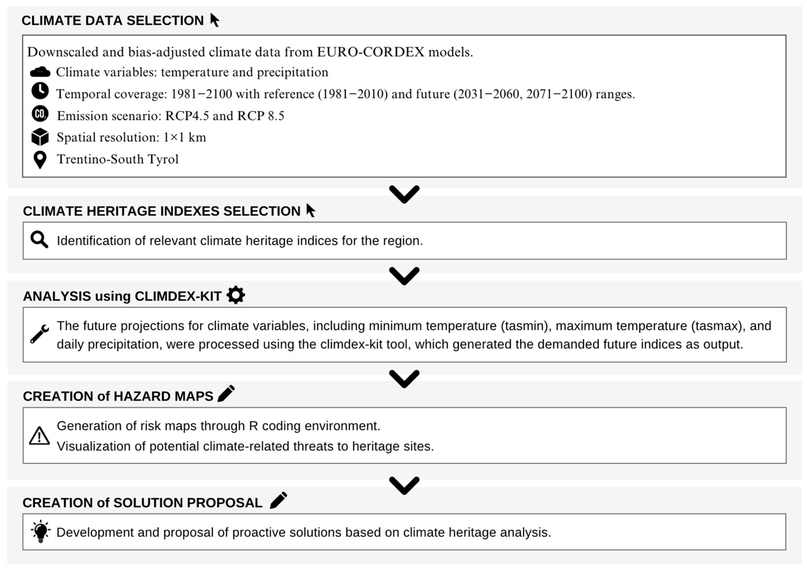
2. Methodology
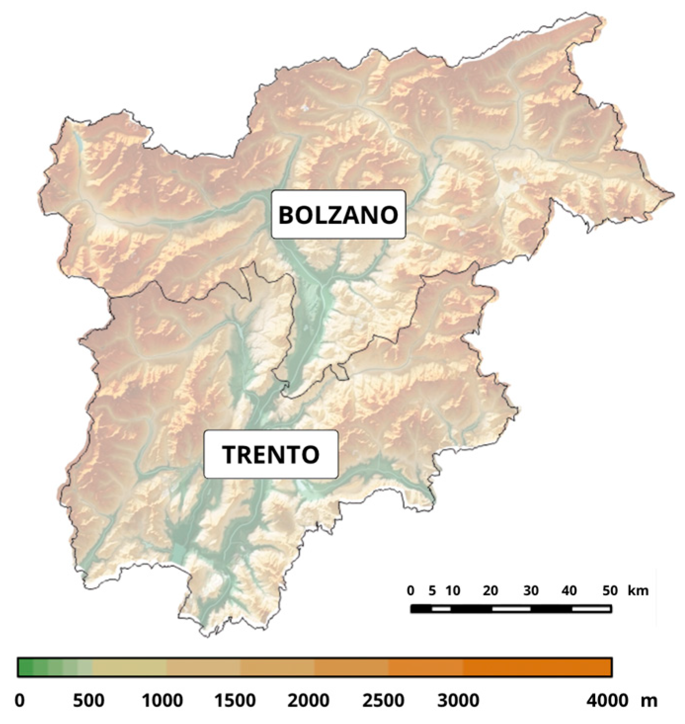
2.1. Target Geographical Area
2.2. Climate-Heritage Indices
- Lichen Species Richness (D);
- Freeze–Thaw Cycles (FTCs);
- Growing Annual Degree Days (GDD15);
- Heavy Precipitation Days with above 10 mm rain (R10);
- Heavy Precipitation Days with above 20 mm rain (R20);
- Wet-Frost Index (WFI);
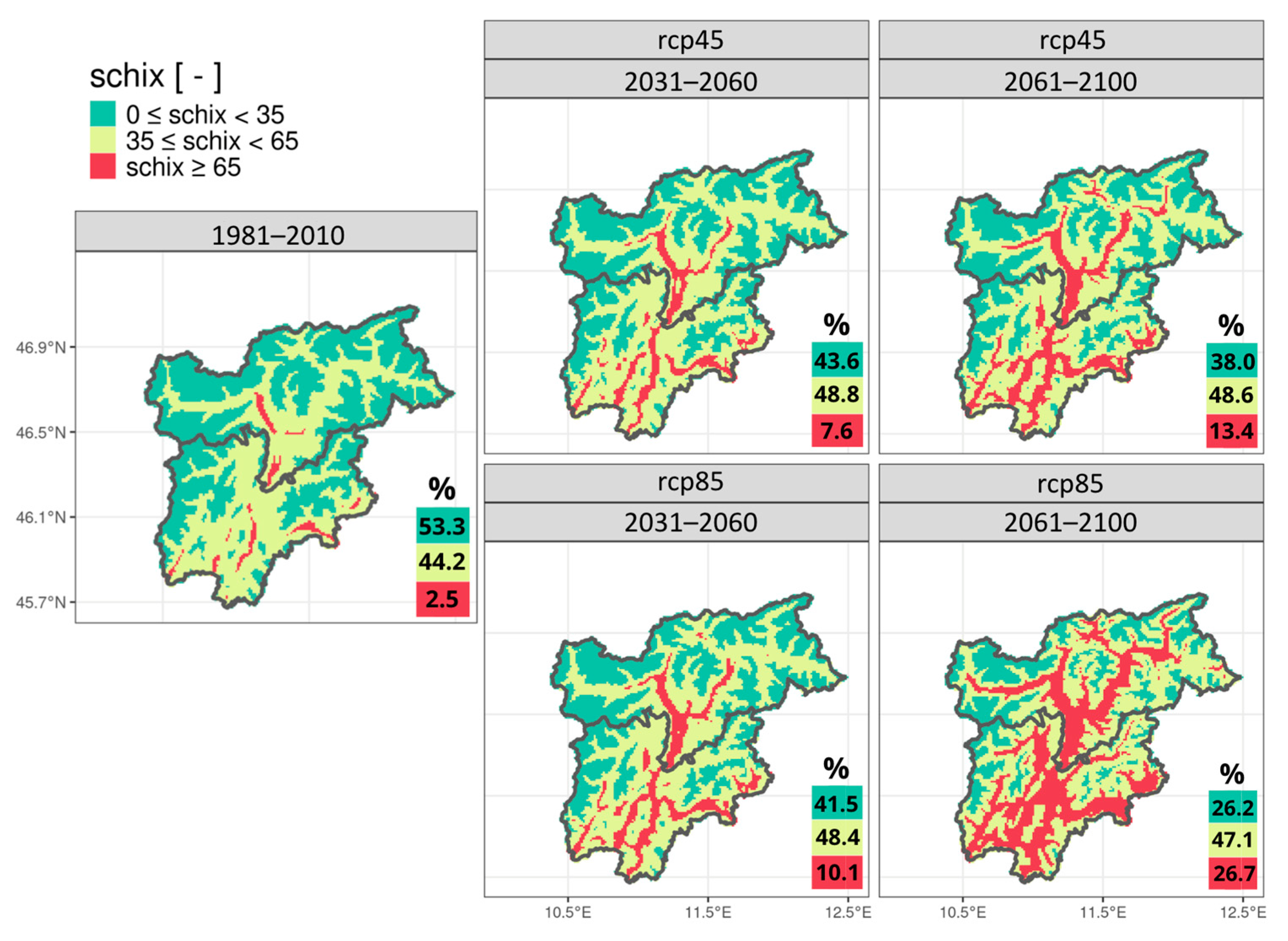
- Scheffer Index (SCHIX);
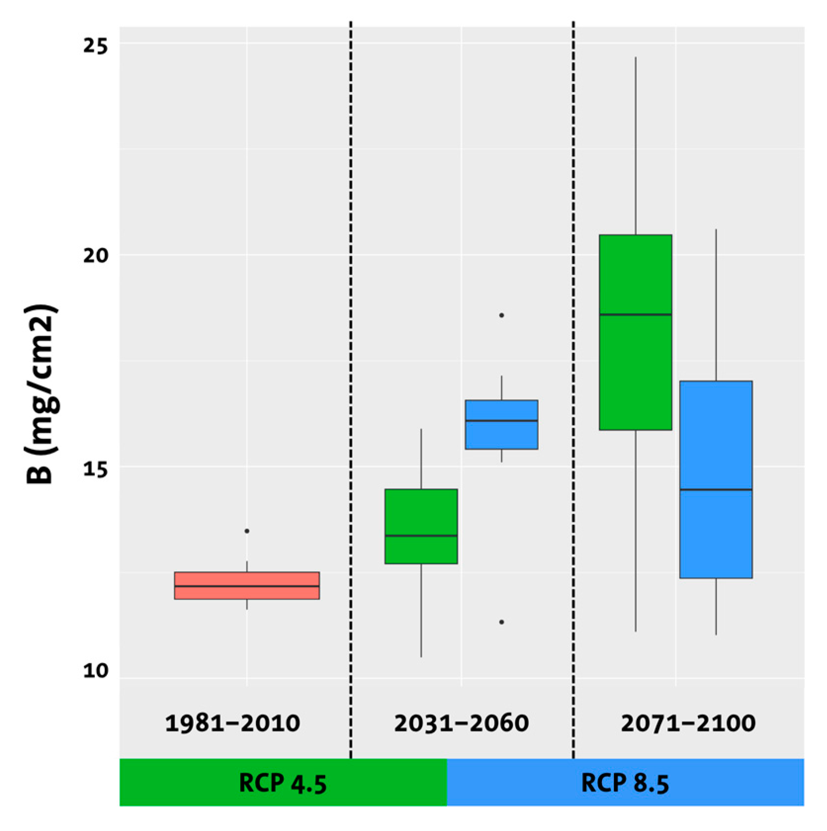
- Biomass Accumulation (B).
2.3. Climate Data
2.4. Future Climate-Heritage Index Calculation
- Maps showing the climatological values of each index;
- Boxplots illustrating the range of projections from different models for each index;
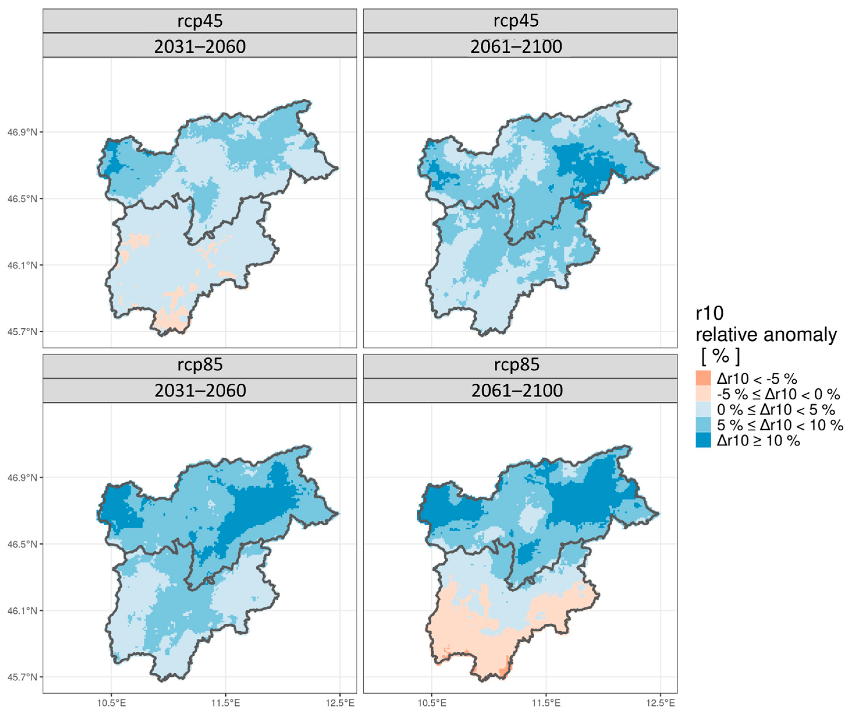
- Maps displaying relative anomalies, which show deviations from the reference period’s climatological averages;
- Additional maps of the climatological values of each index, complemented by an indication of the significance of projected changes under future scenarios, are defined by the agreement among ensemble models. For simplicity, these maps are hereafter referred to as “significance maps”.
3. Results
3.1. Temperature-Derived Indices
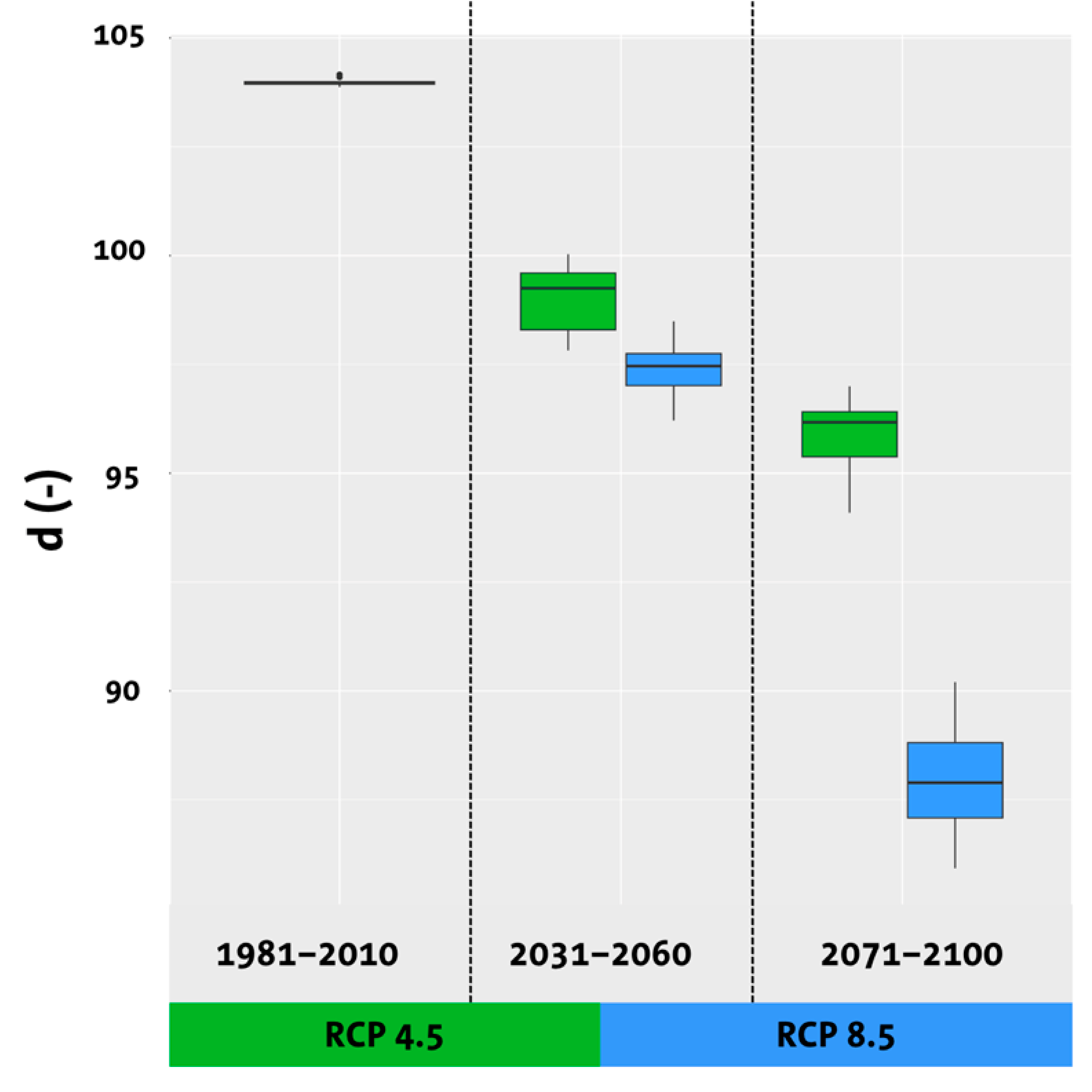
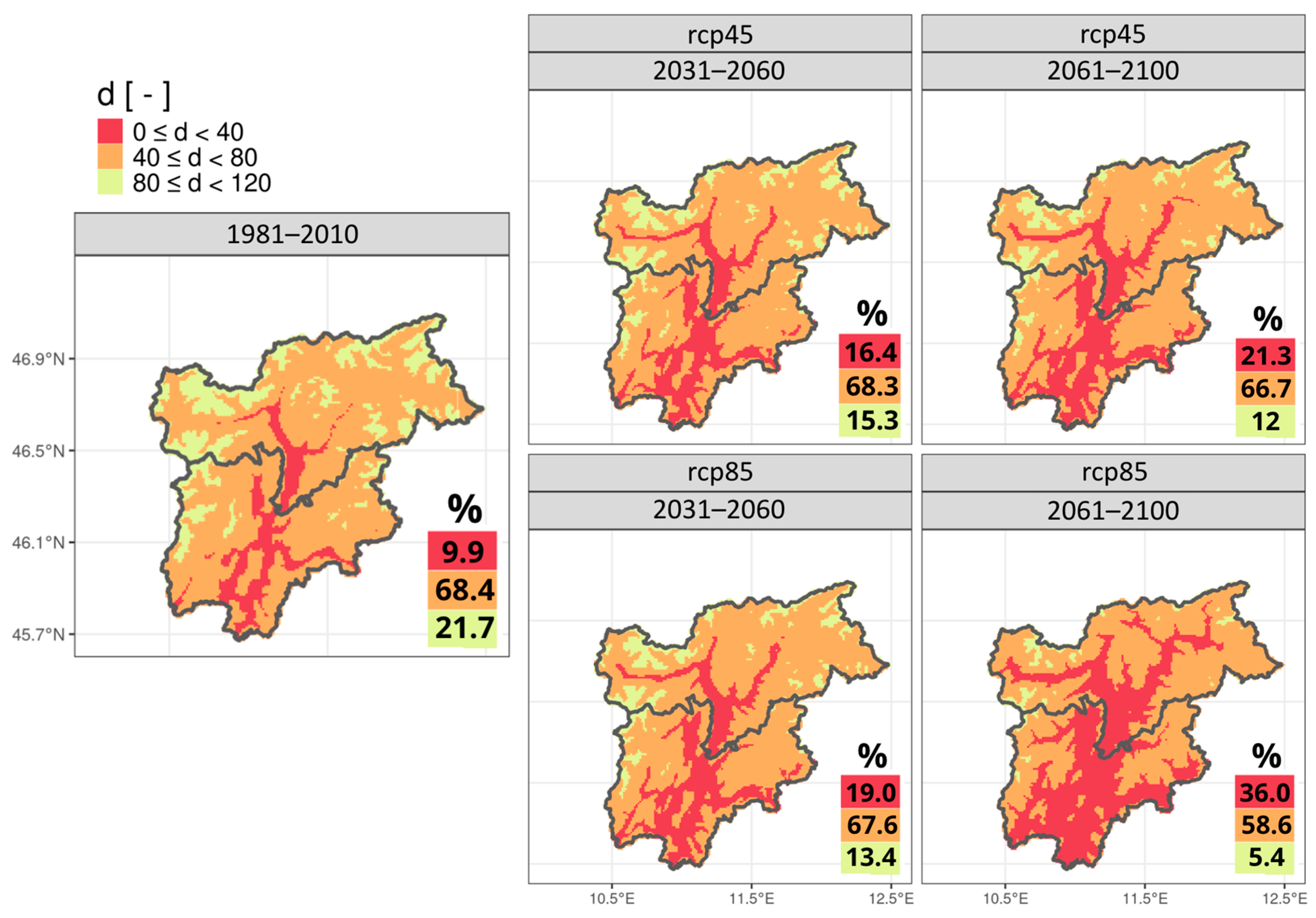
3.1.1. Lichen Species Decay
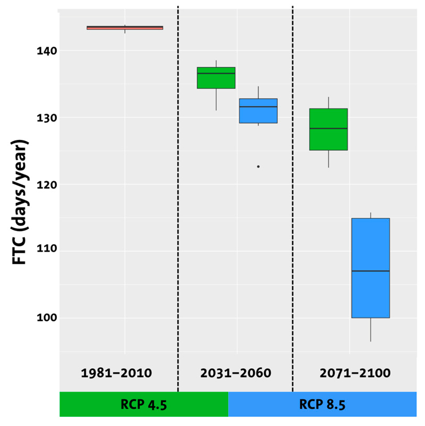
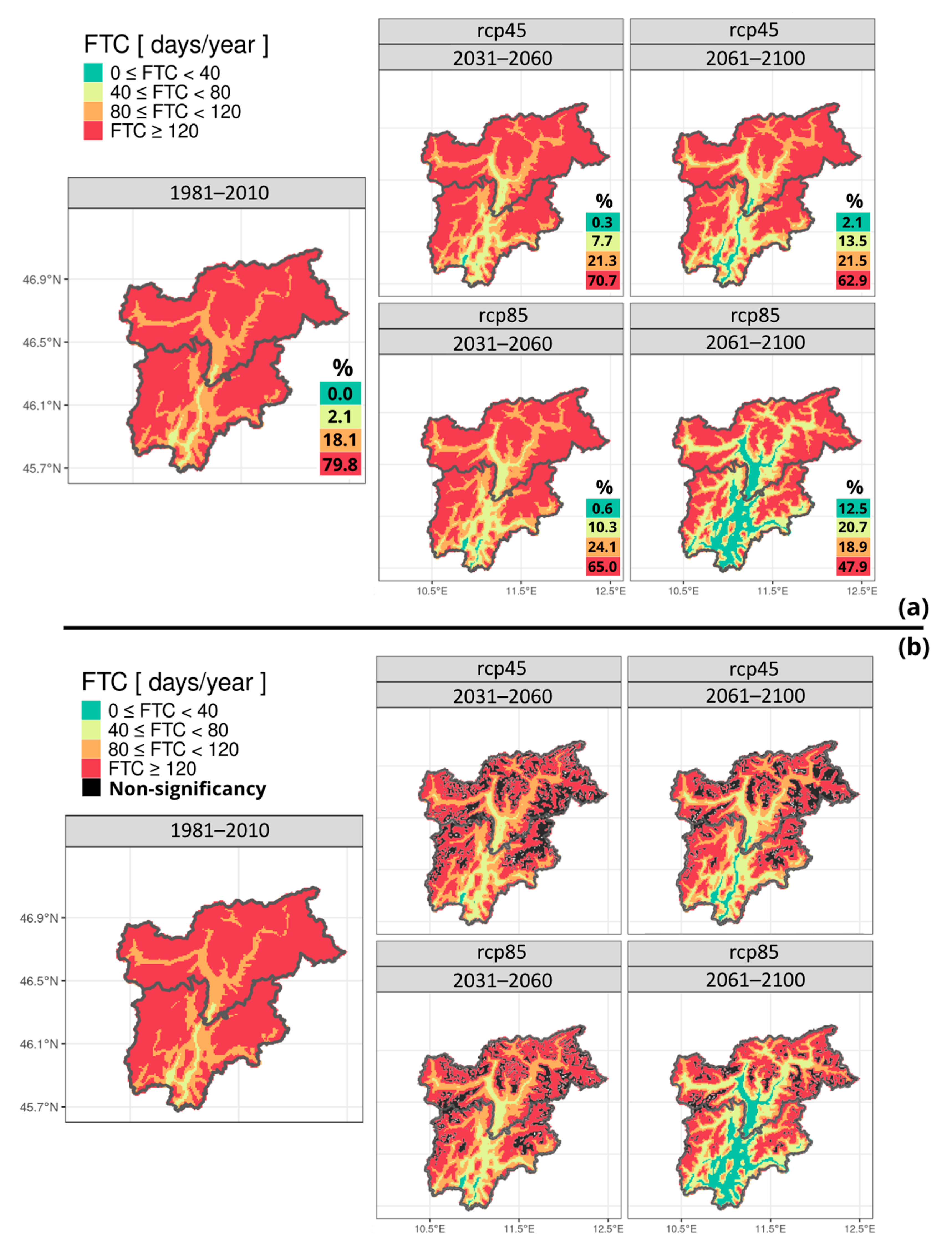
3.1.2. Frost Damages (Freeze–Thaw Cycles, FTCs)
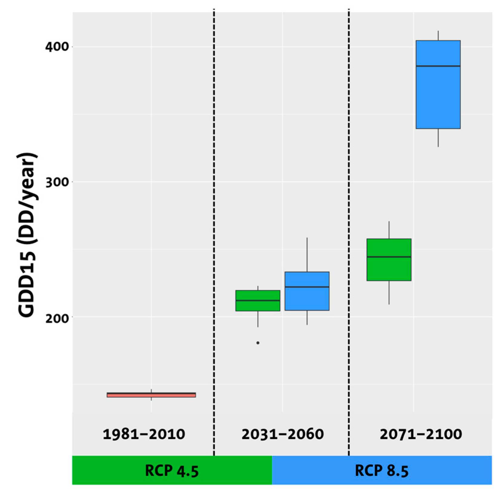
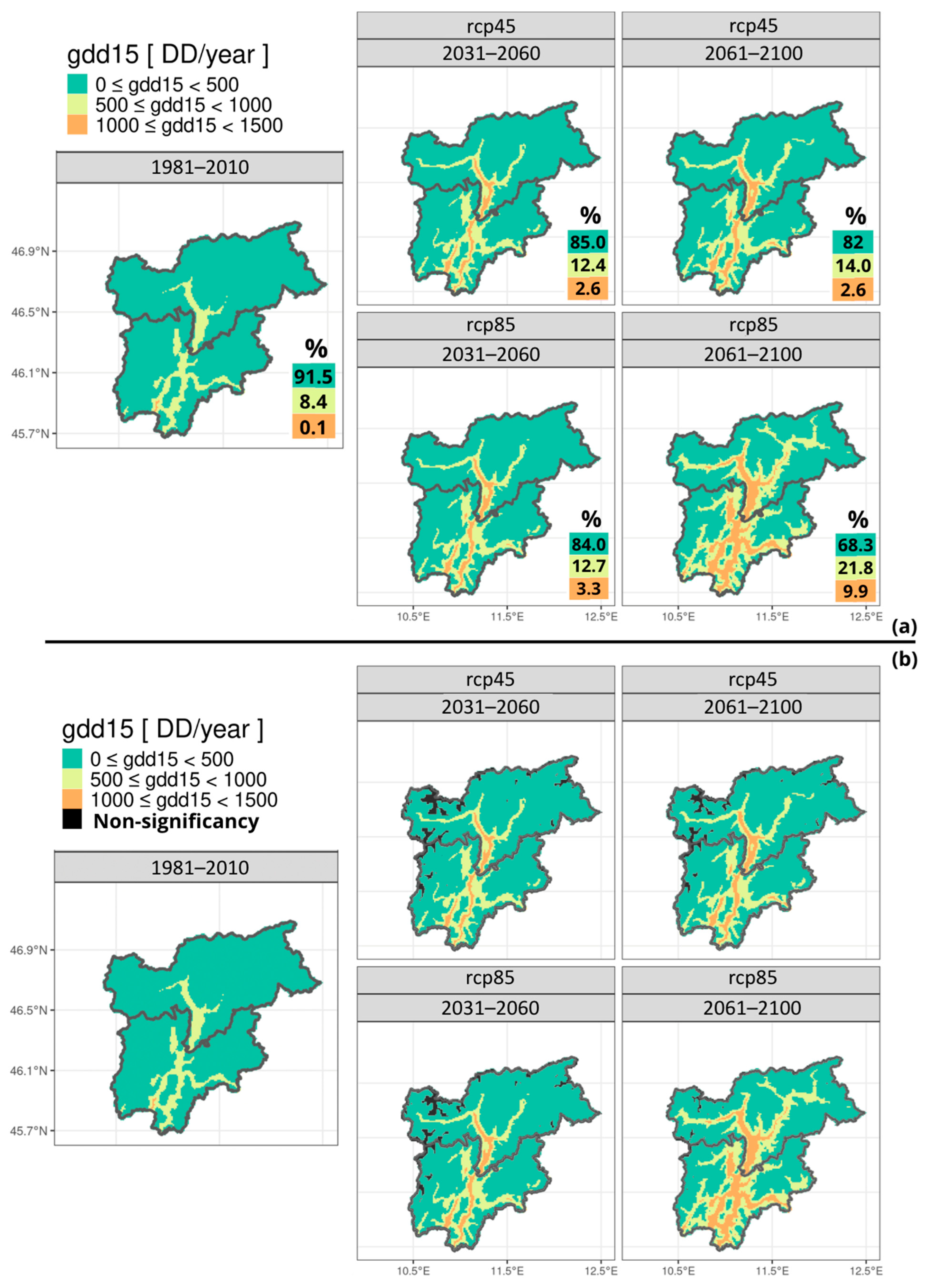
3.1.3. Biological Decay (Temperature-Dependent Insects) on Wood
3.2. Precipitation-Derived Indices
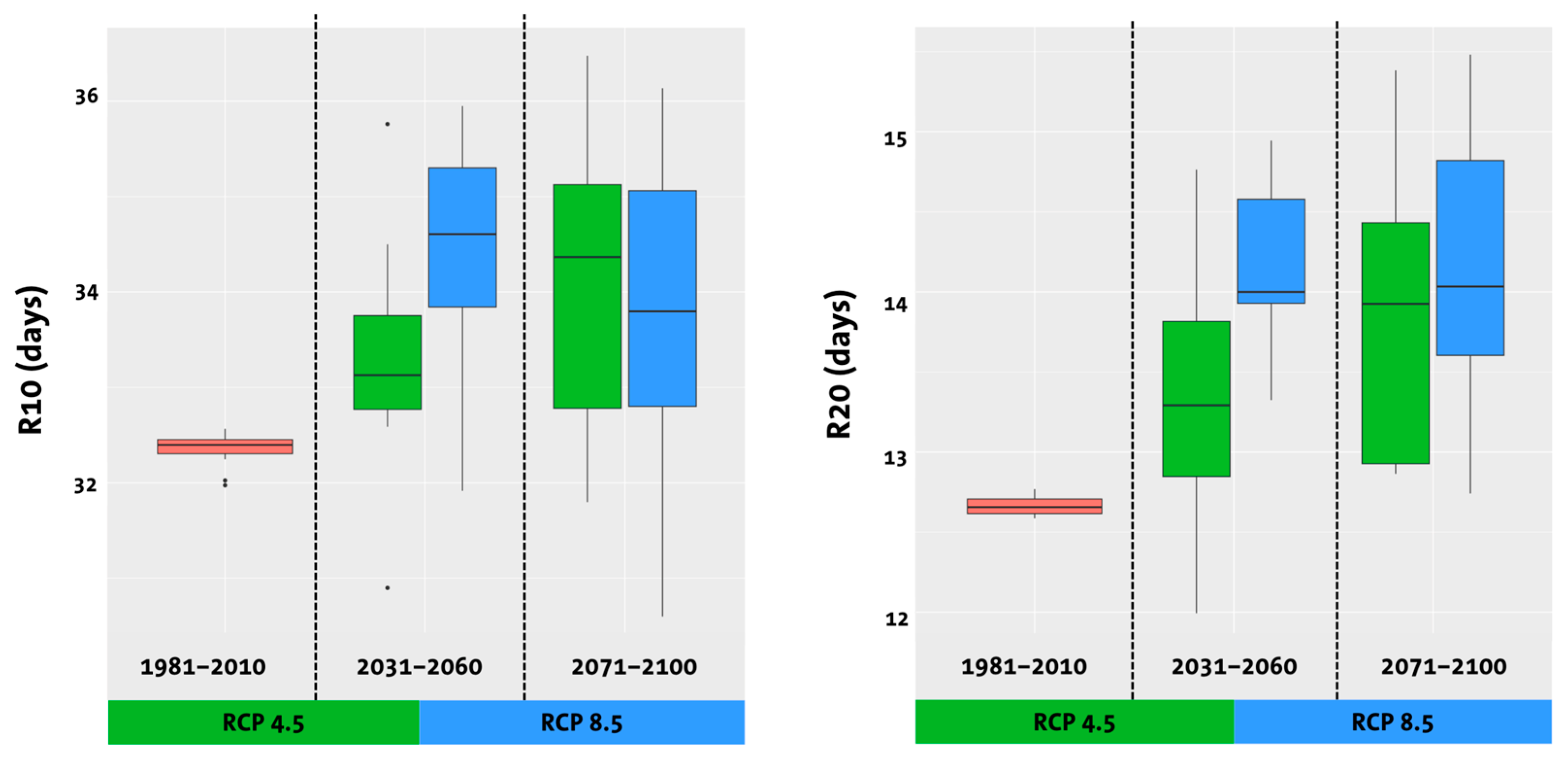
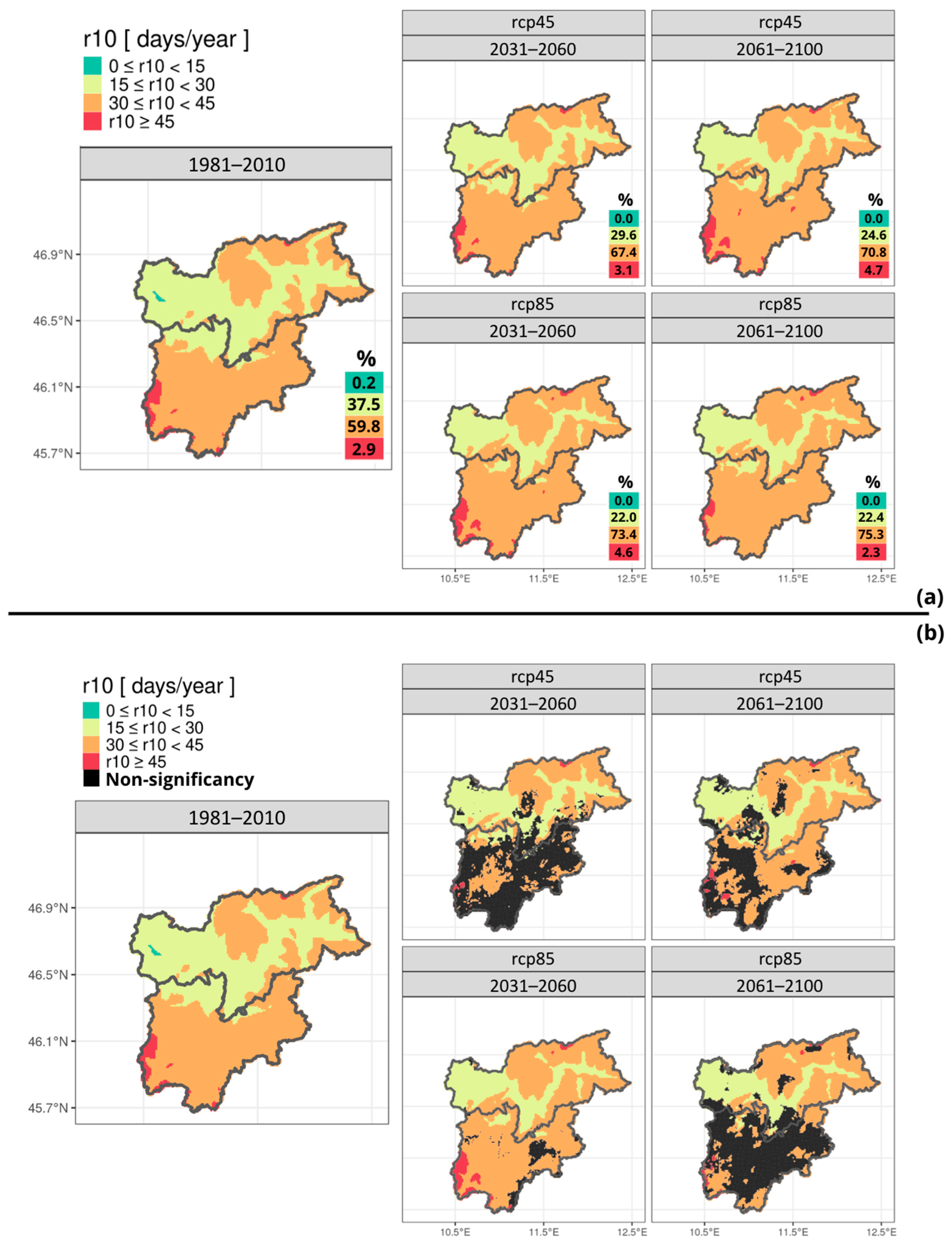
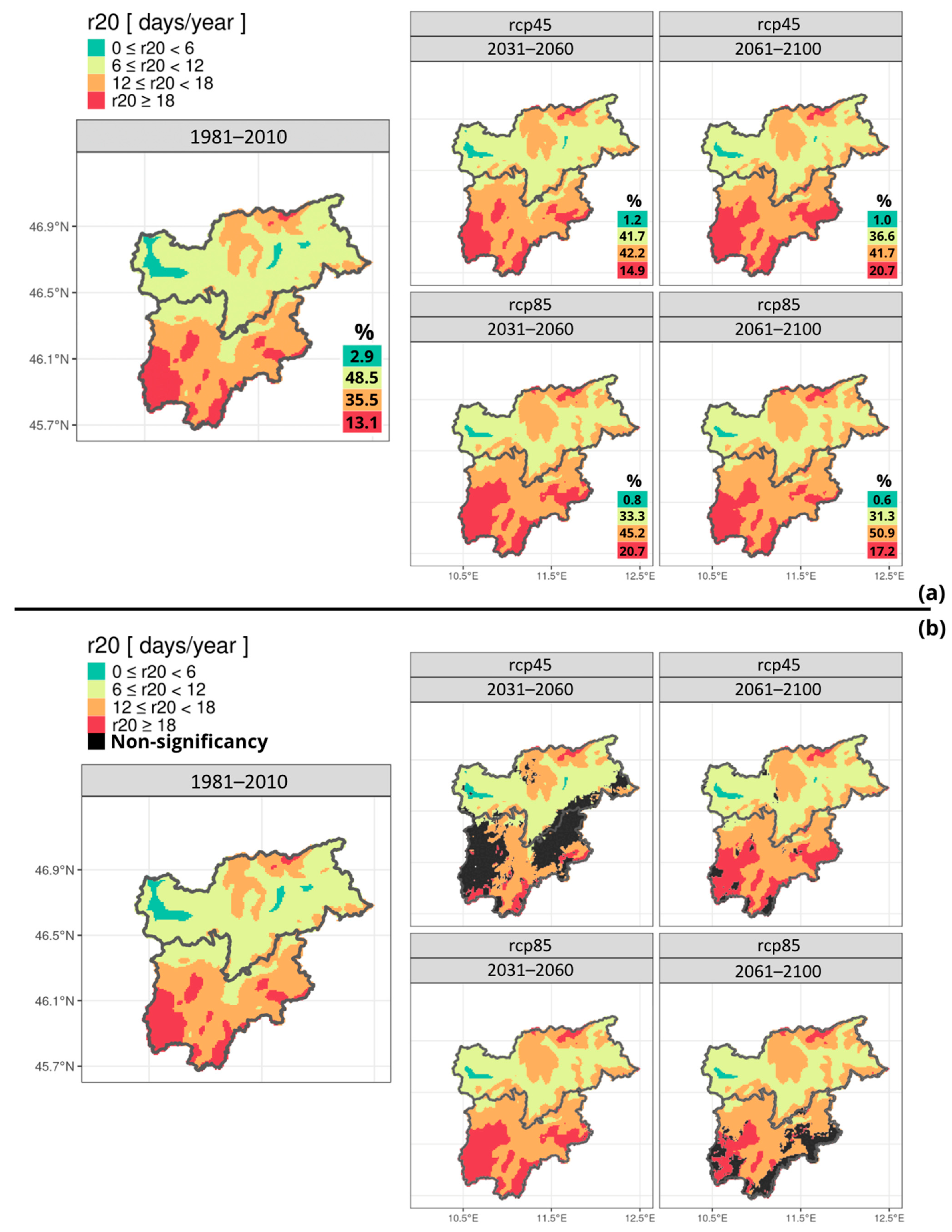
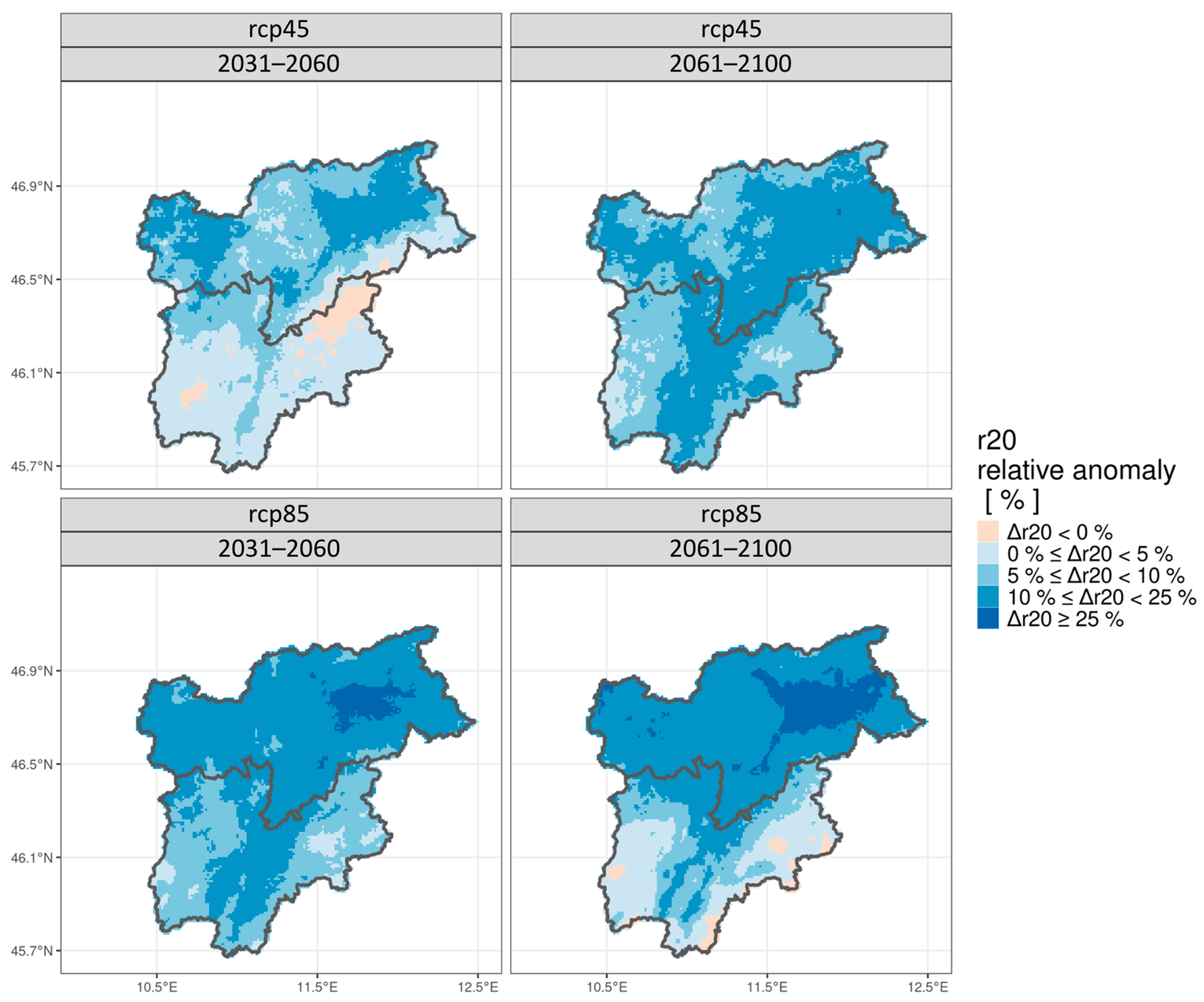
Heavy Precipitation Days (with Pr > 10 mm and Pr > 20 mm)
3.3. Temperature and Precipitation-Derived Indices
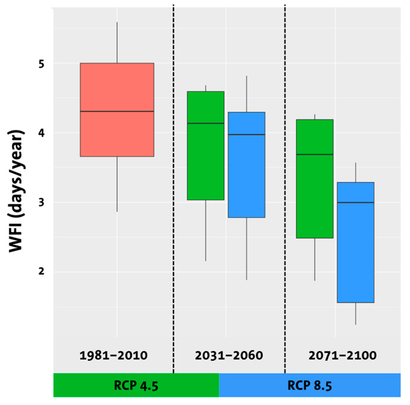
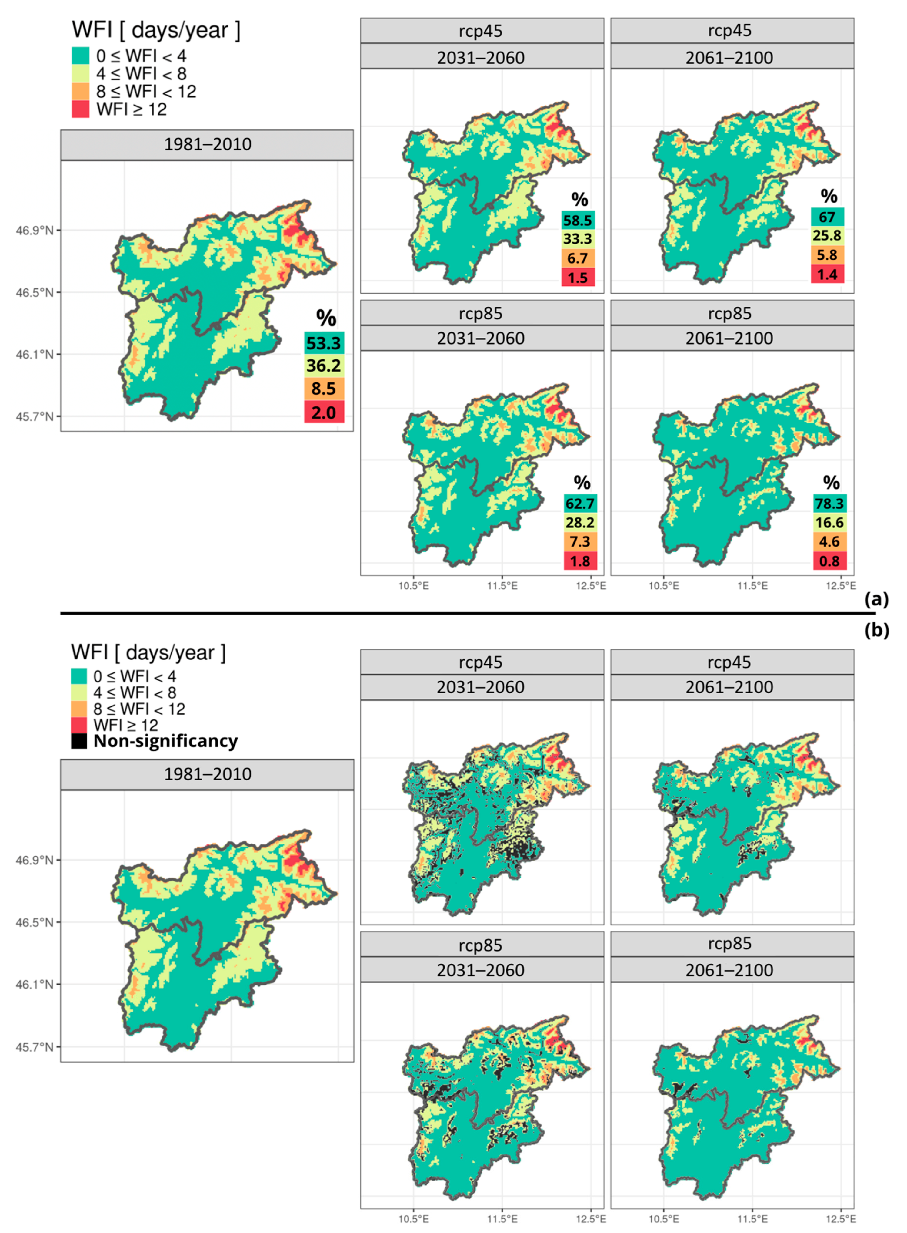
3.3.1. Frost Damages (Wet Frost Index, WFI)
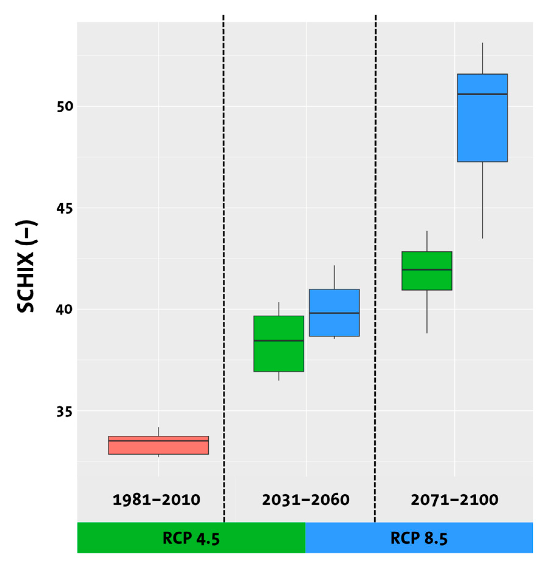
3.3.2. Biological Decay (Fungal) on Wood
3.3.3. Biomass Accumulation
4. Discussion and Proposed Adaptive
5. Conclusions
Supplementary Materials
Author Contributions
Funding
Institutional Review Board Statement
Informed Consent Statement
Data Availability Statement
Acknowledgments
Conflicts of Interest
Abbreviations
| General | |
| Dn | Days with freezing events |
| Dn+1 | Day after |
| Dn−1 | Previous day |
| EURO-CORDEX | Europe Domain Co-Ordinated Regional Downscaling Experiment |
| ETCCDI | Expert Team on Climate Change Detection and Indices |
| GMC | Global Climate Model |
| RCP | Representative Concentration Path |
| RCM | Regional Climate Model |
| Indices | |
| B | Biomass Accumulation [mg/cm2] |
| D | Lichen Species Richness [-] |
| FTC | Freeze–Thaw Cycle [days/year] |
| GDD15 | Growing Degree Days with baseline value 15 °C [degree days/year] |
| R10 | Heavy Precipitation Day with above 10 mm rain [days/year] |
| R20 | Heavy Precipitation Day with above 20 mm rain [days/year] |
| SCHIX | Scheffer Index [-] |
| WFI | Wet-Frost Index [days/year] |
| Variables | |
| P | Daily Precipitation [mm] |
| Py | Yearly Precipitation [mm] |
| Dpr,m,0.2 | Monthly per month with over 0.2 mm of rain [-] |
| Ty,mean | Yearly mean temperature [°C] |
| Tm,mean | Monthly mean temperature [°C] |
| Tas,mean | Daily mean temperature [°C] |
| Tas,max | Daily maximum temperature [°C] |
| Tas,min | Daily minimum temperature [°C] |
Appendix A

| Acronym | Name | Definition | Unity | Possible Change in Historical Building | Formula | Empirical | Existing Benchmark | Index Reference |
|---|---|---|---|---|---|---|---|---|
| Temperature-dependent indices | ||||||||
| D | Lichen species richness | N° of species per monument | - | Aesthetical change | 121.823–4.154 × Ty,mean | YES | NO | [13] |
| FTC | Freeze–thaw cycles | N° of days with maximum T over 0 °C and minimum below 0 °C | days/year | Mechanical deterioration | Tas,max > 0 °C and Tas,min < 0 °C | NO | NO (not for this definition) | [72] |
| GDD15 | Growing annual degree-days | Growing annual degree-days, over 15 °C and below 30 °C for temperature-dependent insects | DD/year | Biological decay (insects) | NO | Low Risk: 0–1000 Medium Risk: 1000–2000 High Risk: 2000–3000 | [47] | |
| Precipitation-dependent indices | ||||||||
| R10 | Heavy precipitation days | N° of days per year with daily precipitation > 10 mm | days/year | Biological and Mechanical deterioration | P > 10 mm | NO | NO | [4] |
| R20 | Heavy precipitation days | N° of days per year with daily precipitation > 20 mm | days/year | Biological and Mechanical deterioration | P > 20 mm | NO | NO | [13] |
| Temperature-Precipitation-dependent indices | ||||||||
| WFI | Wet frost index | N° of days in a year with >2 mm of rain and mean temperature > 0 °C followed immediately by days with mean temperature ≤−3 °C | days/year | Mechanical deterioration | Dn (P > 2 mm and Tas,mean > 0 °C) and Dn+1 (Tas,min ≤ −3 °C) | NO | NO | Author’s Definition |
| SCHIX | Scheffer index | Increase of Tmean by rainy days with more than 0.2 mm of rain | - | Biodecay of wood (insect and fungal attacks) | YES | Low Risk: SCHIX < 35 Medium Risk: 35 < SCHIX < 65 High Risk: SCHIX > 65 | [98] | |
| B | Biomass accumulation | Biomass accumulation on horizontal surfaces | mg/cm2 | Aesthetical change Biological and Mechanical deterioration Protection change from deterioration | YES | NO | [102] | |
| Acronym | Regional Climatology | Regional Relative Change [%] | ||||||||
|---|---|---|---|---|---|---|---|---|---|---|
| RCP 4.5 | RCP 8.5 | RCP 4.5 | RCP 8.5 | |||||||
| Reference | Near Future | Far Future | Reference | Near Future | Far Future | Near Future | Far Future | Near Future | Far Future | |
| D | 104.3 [64.5; 162.5] | 99.5 [59.4; 157.4] | 96.4 [56.5; 154.1] | 104.3 [64.5; 162.5] | 97.8 [58.0; 155.6] | 88.3 [48.8; 145.6] | −4.6 [−7.9; −3.1] | −7.6 [−12.4; −5.2] | −6.2 [−10.1; −4.3] | −15.3 [−24.3; −10.4] |
| FTC | 143.7 [54.4; 209.9] | 136.1 [29.2; 205.1] | 128.4 [19.2; 208.6] | 143.7 [54.5; 210.1] | 131.8 [23.6; 208.1] | 108.6 [3.5; 205.1] | −5.3 [−46.3; −2.3] | −10.7 [−64.7; −0.6] | −8.3 [−56.7; −1.0] | −24.4 [−93.6; −2.4] |
| GDD15 | 140.8 [0; 1045.7] | 209.9 [0; 1218.8] | 239.3 [0; 1300.8] | 140.7 [0; 1045.0] | 218.6 [0; 1265.9] | 377.5 [0; 1425.2] | +49.1 [0.0; +16.6] | +70.0 [0.0; +24.4] | +55.4 [0.0; +21.1] | +168.3 [0.0; +36.4] |
| R10 | 32.4 [14.2; 50.6] | 33.3 [15.6; 50.1] | 34.3 [15.8; 52.1] | 32.5 [14.3; 50.7] | 34.6 [15.9; 52.3] | 34.0 [16.1; 49.0] | +2.8 [+9.9; −1.0] | +5.9 [+11.3; +3.0] | +6.5 [+11.2; +3.2] | +4.6 [+12.6; −3.4] |
| R20 | 12.7 [4.0; 28.0] | 13.3 [4.4; 27.6] | 14.0 [4.7; 29.5] | 12.7 [4.0; 28.0] | 14.2 [4.8; 29.6] | 14.1 [4.9; 27.5] | +4.7 [+10.0; −1.4] | +10.2 [+17.5; +5.4] | +11.8 [+20.0; +5.7] | +11.0 [+22.5; −1.8] |
| WFI | 4.3 [0.3; 19.0] | 3.9 [0.1; 18.2] | 3.4 [0.0; 19.0] | 4.3 [0.3; 19.4] | 3.7 [0.1; 18.6] | 2.6 [0.0; 16.1] | −9.3 [−66.7; −4.2] | −20.9 [−100.0; 0.0] | −14.0 [−66.7; −4.12] | −39.5 [−100.0; −17.0] |
| SCHIX | 32.9 [0.1; 77.8] | 38.1 [0.1; 84.4] | 41.5 [0.1; 89.7] | 33.1 [0.1; 78.5] | 39.6 [0.1; 86.5] | 49.8 [1.1; 86.5] | +15.8 [0.0; +8.5] | +26.1 [0.0; +15.3] | +19.6 [0.0; +10.2] | +50.45 [+1000.0;+10.9] |
| B | 12.2 [1.8; 90.3] | 13.4 [1.9; 100.5] | 18.2 [2.0; 225.5] | 12.3 [1.8; 102.1] | 16.0 [2.0; 118.9] | 14.4 [1.9; 104.8] | +9.8 [+5.6; +11.3] | +49.2 [+11.1; +149.7] | +30.1 [+11.1; +16.5] | +17.1 [+5.6; +2.6] |
| Indices | Results | Consequencies | Solutions |
|---|---|---|---|
| Lichen Species Richness (D) | General decrease in valleys; Far Future (RCP 4.5): decrease reaches also narrow valleys; Far Future (RCP 8.5): decrease affects also small altitudes. | Decrease of biodiversity; Change in aesthetics; Change in degradation/protection role of lichens | Planting Vegetation |
| Growing Degree Days (GDD) | Increase in valleys | Increase in wood attacking insects | Removal of close trees |
| Freeze–Thawing Cycles (FTC) | Decrease in valleys | Decrease in frost damages | Soft capping for horizontal stone surfaces; Vegetation capping for fountains; Solid Enclosings for fountains; Flexible enclosings for statues; Shading shelters for archaeological sites. |
| Heavy Precipitation Days 1 (R10) | General increase | Increase in biological and mechanical deterioration e.g., deep penetration, salt crystallization, mould, stone recession, etc. | Roof and soil drainage system redesign and maintenance; Façade detail augmentation or adding; Installation of rodding point, wire balloons, grille-covered gulley traps and french drains; Application of waterproofing coatings; Installation of EPGs. |
| Heavy Precipitation Days 2 (R20) | General increase | Increase in biological and mechanical deterioration e.g., deep penetration, salt crystallization, mould, stone recession, etc. | Same as in R10 |
| Wet-Frost Index (WTI) | Small general decrease, with high uncertainties | Small decrease in frost damages | Same as in FTC |
| Scheffer Index (SCHIX) | General high increase; Shift from least favourable-intermediate to intermediate-most favourable conductive condition for wood decay. | Increase of decay hazard induced by wood-degrading fungi on wooden elements. | Specialised coatings; Avoid humidity/water absorbtion. |
| Biomass Accumulation (B) | General increase | Change in aesthetics; Change in biochemical role of biomass. | Cleaning of surfaces; Specialised coatings. |
References
- Sesana, E.; Gagnon, A.S.; Ciantelli, C.; Cassar, J.; Hughes, J. Climate Change Impacts on Cultural Heritage: A Literature Review. Wiley Interdiscip. Rev. Clim. Chang. 2021, 12, e710. [Google Scholar] [CrossRef]
- Lefèvre, R.-A. Lefèvre, R.-A. Le Patrimoine Culturel Dans Le Plan National Français d’Adaptation Au Changement Climatique. In Cultural Heritage Facing Climate Change: Experiences and Ideas for Resilience and Adaptation; Lefèvre, R.-A., Sabbioni, C., Eds.; Edipuglia: Ravello, Italy, 2018. [Google Scholar]
- Caldas, A.; Lafrenz Samuels, K.; Markham, A.; Osipova, E. World Heritage and Tourism in a Changing Climate; UNESCO Publishing: Paris, France; Nairobi, Kenya; Cambridge, MA, USA, 2016. [Google Scholar]
- Brimblecombe, P.; Grossi Sampedro, C.M.; Harris, I. Climate Change Critical to Cultural Heritage. In Proceedings of the International Conference on Heritage, Weathering and Conservation, Madrid, Spain, 21–24 June 2006; Volume 1, pp. 387–393. [Google Scholar]
- Ashley-Smith, J. Damage functions. In Climate for Culture: Built Cultural Heritage in Times of Climate Change; Frauenhofer ISI Publisher: Brussels, Belgium, 2014; Available online: https://www.isi.fraunhofer.de/content/dam/isi/dokumente/w/2024/2015_ClimateforCulture_Brochure.pdf (accessed on 1 June 2025).
- Blavier, C.L.S.; Huerto-Cardenas, H.E.; Aste, N.; Del Pero, C.; Leonforte, F.; Della Torre, S. Adaptive Measures for Preserving Heritage Buildings in the Face of Climate Change: A Review. Build. Environ. 2023, 245, 110832. [Google Scholar] [CrossRef]
- Ministero dell’Ambiente e della Sicurezza Energetica PNACC. Allegato Ii, Metodologie per La Definizione Di Strategie e Piani Locali Di Adattamento Ai Cambiamenti Climatici; Ministero dell’Ambiente e della Sicurezza Energetica Publisher: Rome, Italy, 2023. [Google Scholar]
- European Commission. COM(2021) 82 Final: Forging a Climate-Resilient Europe—The New EU Strategy on Adaptation to Climate Change; European Commission: Brussels, Belgium, 2021. [Google Scholar]
- Ministero dell’ambiente e della tutela del territorio e del mare. Strategia Nazionale Di Adattamento Ai Cambiamenti Climatici (SNAC); Ministero dell’Ambiente e della Sicurezza Energetica: Rome, Italy, 2015. [Google Scholar]
- Governo italiano. Piano Nazionale Di Ripresa e Resilienza (PNRR); Domani: Rome, Italy, 2021. [Google Scholar]
- Ministero dell’Ambiente e della Sicurezza Energetica. Piano Nazionale Di Adattamento Ai Cambiamenti Climatici; Ministero dell’Ambiente e della Sicurezza Energetica: Rome, Italy, 2022. [Google Scholar]
- ISPRA. Dissesto Idrogeologico in Italia: Pericolosità e Indicatori Di Rischio Edizione 2021; SNPA: Roma, Italy, 2021. [Google Scholar]
- Cassar, M.; Sabbioni, C.; Brimblecombe, P. The Atlas of Climate Change Impact on European Cultural Heritage: Scientific Analysis and Management Strategies; Cassar, M., Sabbioni, C., Brimblecombe, P., Eds.; Anthem Press: London, UK, 2010. [Google Scholar]
- IPCC. Climate Change 2001: Impacts, Adaptation and Vulnerability, IPCC Working Group II, Technical Summary; Cambridge University Press: Cambridge, UK, 2001. [Google Scholar]
- Leveghi, D. E’ in Alto Adige il Comune Dove Sono Aumentate di più le Temperature in 50 Anni. Trentino Alto Adige Seconda Regione in Italia Per Surriscaldamento; Il Dolomiti: Trento, Italy, 2020. [Google Scholar]
- Niedrist, G.; Zebisch, M.; Crespi, A.; Iacopino, T.; Fritsch, U.; Barandun, M.; Bertoldi, G.; Bottarin, R.; Hoffmann, C.; Jacob, A.; et al. Climate Change Monitoring South Tyrol. Available online: https://www.eurac.edu/doi/10-57749-8zpx-hm12 (accessed on 5 August 2024).
- Vincoli in Rete. Available online: http://vincoliinrete.beniculturali.it/VincoliInRete/vir/bene/ricercabeni (accessed on 23 May 2024).
- Brischke, C.; Selter, V. Mapping the Decay Hazard of Wooden Structures in Topographically Divergent Regions. Forests 2020, 11, 510. [Google Scholar] [CrossRef]
- Adler, S.; Chimani, B.; Drechsel, S.; Haslinger, K.; Hiebl, J.; Meyer, V.; Resch, G.; Rudolph, J.; Vergeiner, J.; Zingerle, C.; et al. Il clima del Tirolo-Alto Adige-Bellunese. 2015. Available online: http://www.clima-alpino.eu/images/Il_clima_del_Tirolo-Alto_Adige-Bellunese.pdf (accessed on 1 June 2025).
- Ministero dell’Ambiente e della Tutela del Territorio e del Mare. PNACC-Allegato III-Impatti e Vulnerabilità Settoriali; Ministero dell’Ambiente e della Sicurezza Energetica: Rome, Italy, 2018. [Google Scholar]
- Crespi, A.; Matiu, M.; Bertoldi, G.; Petitta, M.; Zebisch, M. A High-Resolution Gridded Dataset of Daily Temperature and Precipitation Records (1980-2018) for Trentino-South Tyrol (North-Eastern Italian Alps). Earth Syst. Sci. Data Discuss. 2021, 13, 2801–2818. [Google Scholar] [CrossRef]
- Campalani, P.; Crespi, A.; Pittore, M.; Zebisch, M. Climdex-Kit: An Open Software for Climate Index Calculation, Sharing and Analysis towards Tailored Climate Services. Environ. Model. Softw. 2025, 190, 106442. [Google Scholar] [CrossRef]
- Brimblecombe, P.; Richards, J. Applied Climatology for Heritage. Theor. Appl. Climatol. 2024, 155, 7325–7333. [Google Scholar] [CrossRef]
- Bertoldi, G.; Bozzoli, M.; Crespi, A.; Matiu, M.; Giovannini, L.; Zardi, D.; Majone, B. Diverging Snowfall Trends across Months and Elevation in the Northeastern Italian Alps. Int. J. Climatol. 2023, 43, 2794–2819. [Google Scholar] [CrossRef]
- Hao, L.; Herrera-Avellanosa, D.; Del Pero, C.; Troi, A. Categorization of South Tyrolean Built Heritage with Consideration of the Impact of Climate. Climate 2019, 7, 139. [Google Scholar] [CrossRef]
- Eccel, E.; Saibanti, S. Inquadramento Climatico Dell’Altopiano Di Lavarone-Vezzena Nel Contesto Generale Trentino. Acta Geol. 2005, 82, 111–121. [Google Scholar]
- Spatial Analysis of Climate. Available online: http://www.3pclim.eu/index.php?option=com_content&view=article&id=227&catid=9&Itemid=244&lang=en (accessed on 5 September 2024).
- Agenzia Provinciale per la Protezione dell’Ambiente (APPA). I Cambiamenti Climatici in Trentino. Osservazioni, Scenari Futuri e Impatti; APPA: Trento, Italy, 2022. [Google Scholar]
- Vandemeulebroucke, I.; Kotova, L.; Caluwaerts, S.; Van Den Bossche, N. Degradation of Brick Masonry Walls in Europe and the Mediterranean: Advantages of a Response-Based Analysis to Study Climate Change. Build. Environ. 2023, 230, 109963. [Google Scholar] [CrossRef]
- Vyshkvarkova, E.; Sukhonos, O. Climate Change Impact on the Cultural Heritage Sites in the European Part of Russia over the Past 60 Years. Climate 2023, 11, 50. [Google Scholar] [CrossRef]
- Sabbioni, C.; Brimblecombe, P.; Lefevre, R.A. European and Mediterranean Major Hazards Agreement (EUR-OPA) Vulnerability of Cultural Heritage to Climate Change; Council of Europe Publisher: Strasbourg, France, 2008; Volume 44. [Google Scholar]
- Sabbioni, C.; Bonazza, A. How Mapping Climate Change for Cultural Heritage? The Noah’s Ark Project. In Climate Change and Cultural Heritage; Edipuglia: Bari, Italy, 2009; pp. 37–41. [Google Scholar]
- Frauenhofer Institute Climate for Culture. Available online: https://www.climateforculture.eu/ (accessed on 28 September 2022).
- Expert Team on Climate Change Detection and Indices (ETCCDI). ETCCDI Climate Change Indices. Available online: https://etccdi.pacificclimate.org/list_27_indices.shtml (accessed on 1 June 2025).
- McIlroy de la Rosa, J.P.; Casares Porcel, M.; Warke, P.A. Mapping Stone Surface Temperature Fluctuations: Implications for Lichen Distribution and Biomodification on Historic Stone Surfaces. J. Cult. Herit. 2013, 14, 346–353. [Google Scholar] [CrossRef]
- Sardella, A.; Palazzi, E.; von Hardenberg, J.; Del Grande, C.; De Nuntiis, P.; Sabbioni, C.; Bonazza, A. Risk Mapping for the Sustainable Protection of Cultural Heritage in Extreme Changing Environments. Atmosphere 2020, 11, 700. [Google Scholar] [CrossRef]
- Bonazza, A.; Sardella, A. Climate Change and Cultural Heritage: Methods and Approaches for Damage and Risk Assessment Addressed to a Practical Application. Heritage 2023, 6, 3578–3589. [Google Scholar] [CrossRef]
- Clark, J.; Littell, J.S.; Alder, J.R.; Teats, N. Exposure of Cultural Resources to 21st-Century Climate Change: Towards a Risk Management Plan. Clim. Risk Manag. 2022, 35, 100385. [Google Scholar] [CrossRef]
- ISPRA. CARG—Cartografia Geologica e Geotematica; SNPA: Roma, Italy, 2023. Available online: https://www.isprambiente.gov.it/it/progetti/cartella-progetti-in-corso/suolo-e-territorio-1/progetto-carg-cartografia-geologica-e-geotematica (accessed on 1 June 2025).
- Masson-Delmotte, V.; Zhai, P.; Pirani, A.; Connors, S.L.; Péan, C.; Berger, S.; Caud, N.; Chen, Y.; Goldfarb, L.; Gomis, M.I.; et al. IPCC, 2021: Climate Change 2021: The Physical Science Basis. Contribution of Working Group I to the Sixth Assessment Report of the Intergovernmental Panel on Climate Change; Intergovernmental Panel on Climate Change (IPCC) Publisher: Geneva, Switzerland, 2021. [Google Scholar]
- European Environment Agency and European Commission Extreme Precipitation Days. Available online: https://climate-adapt.eea.europa.eu/en/metadata/indicators/extreme-precipitation-days (accessed on 21 July 2024).
- Copernicus Climate Change Service (C3S). C.D.S. CORDEX Regional Climate Model Data on Single Levels. Copernicus. Available online: https://cds.climate.copernicus.eu/datasets/projections-cordex-domains-single-levels?tab=download (accessed on 1 June 2025).
- Jacob, D.; Petersen, J.; Eggert, B.; Alias, A.; Christensen, O.B.; Bouwer, L.M.; Braun, A.; Colette, A.; Déqué, M.; Georgievski, G.; et al. EURO-CORDEX: New High-Resolution Climate Change Projections for European Impact Research. Reg. Environ. Chang. 2014, 14, 563–578. [Google Scholar] [CrossRef]
- Parker, W.S. Ensemble Modeling, Uncertainty and Robust Predictions. WIREs Clim. Chang. 2013, 4, 213–223. [Google Scholar] [CrossRef]
- Schulzweida, U. CDO User Guide. 2021. Available online: https://it.scribd.com/document/466663264/cdo (accessed on 1 June 2025).
- RStudio Team. RStudio: Integrated Development Environment for R; RStudio, PBC: Boston, MA, USA, 1993; Available online: https://posit.co/products/open-source/rstudio/ (accessed on 1 June 2025).
- Loli, A.; Bertolin, C. Indoor Multi-Risk Scenarios of Climate Change Effects on Building Materials in Scandinavian Countries. Geosciences 2018, 8, 347. [Google Scholar] [CrossRef]
- Scheffer, T. A Climate Index for Estimating Potential for Decay in Wood Structures above Ground. For. Prod. J. 1971, 6, 25–31. [Google Scholar]
- Pinna, D. Biofilms and Lichens on Stone Monuments: Do They Damage or Protect? Front. Microbiol. 2014, 5, 133. [Google Scholar] [CrossRef]
- Ariño, X.; Ortega-Calvo, J.J.; Gomez-Bolea, A.; Saiz-Jimenez, C. Lichen Colonization of the Roman Pavement at Baelo Claudia (Cadiz, Spain): Biodeterioration vs. Bioprotection. Sci. Total Environ. 1995, 167, 353–363. [Google Scholar] [CrossRef]
- Sterflinger, K. Temperature and NaCl- Tolerance of Rock-Inhabiting Meristematic Fungi. Antonie van Leeuwenhoek 1998, 74, 271–281. [Google Scholar] [CrossRef] [PubMed]
- Cuzman, O.; Olmi, R.; Riminesi, C.; Tiano, P. Preliminary Study on Controlling Black Fungi Dwelling on Stone Monuments by Using a Microwave Heating System. Int. J. Conserv. Sci. 2013, 4, 133–144. [Google Scholar]
- Tretiach, M.; Bertuzzi, S.; Candotto Carniel, F. Heat Shock Treatments: A New Safe Approach against Lichen Growth on Outdoor Stone Surfaces. Environ. Sci. Technol. 2012, 46, 6851–6859. [Google Scholar] [CrossRef]
- Gomez-Bolea, A.; Peña Rabadán, J.C. Bioprotection of Stone Monuments under Warmer Atmosphere. In Cultural Heritage Facing Climate Change: Experiences and Ideas for Resilience and Adaptation; Edipuglia, Ed.: Bari, Italy, 2018; pp. 65–73. [Google Scholar]
- Palmer, F.E.; Staley, J.T.; Ryan, B. Ecophysiology of Microcolonial Fungi and Lichens on Rocks in Northeastern Oregon. New Phytol. 1990, 116, 613–620. [Google Scholar] [CrossRef]
- Curtis, R.; Jenkins, M.; Snow, J. Short Guide: Maintaining Your Home; Historic Scotland: Edinburgh, UK, 2014. [Google Scholar]
- Everett, D.H. The Thermodynamics of Frost Damage to Porous Solids. Trans. Faraday Soc. 1961, 57, 1541–1551. [Google Scholar] [CrossRef]
- Deprez, M.; De Kock, T.; De Schutter, G.; Cnudde, V. A Review on Freeze-Thaw Action and Weathering of Rocks. Earth Sci. Rev. 2020, 203, 103143. [Google Scholar] [CrossRef]
- Honeyborne, D.B. Weathering and Decay of Masonry. In Conservation of Building and Decorative Stone; Routledge: London, UK, 2007; pp. 153–178. [Google Scholar]
- Nelson, F.E.; Anisimov, O.A.; Shiklomanov, N.I. Subsidence Risk from Thawing Permafrost. Nature 2001, 410, 889–890. [Google Scholar] [CrossRef]
- Nelson, F.E.; Anisimov, O.A.; Shiklomanov, N.I. Climate Change and Hazard Zonation in the Circum-Arctic Permafrost Regions. Nat. Hazards 2002, 26, 203–225. [Google Scholar] [CrossRef]
- Humlum, O.; Instanes, A.; Sollid, J.L. Permafrost in Svalbard: A Review of Research History, Climatic Background and Engineering Challenges. Polar Res. 2003, 22, 191–215. [Google Scholar] [CrossRef]
- Hinzman, L.D.; Bettez, N.D.; Bolton, W.R.; Chapin, F.S.; Dyurgerov, M.B.; Fastie, C.L.; Griffith, B.; Hollister, R.D.; Hope, A.; Huntington, H.P.; et al. Evidence and Implications of Recent Climate Change in Northern Alaska and Other Arctic Regions. Clim. Chang. 2005, 72, 251–298. [Google Scholar] [CrossRef]
- Harris, C.; Rea, B.; Davies, M. Scaled Physical Modelling of Mass Movement Processes on Thawing Slopes. Permafr. Periglac. Process. 2001, 12, 125–135. [Google Scholar] [CrossRef]
- Harris, C.; Vonder Mühll, D.; Isaksen, K.; Haeberli, W.; Sollid, J.L.; King, L.; Holmlund, P.; Dramis, F.; Guglielmin, M.; Palacios, D. Warming Permafrost in European Mountains. Glob. Planet. Change 2003, 39, 215–225. [Google Scholar] [CrossRef]
- Brimblecombe, P.; Grossi, C.M.; Harris, I. Climate Change Critical to Cultural Heritage. In Survival and Sustainability: Environmental Concerns in the 21st Century; Gökçekus, H., Türker, U., LaMoreaux, J.W., Eds.; Springer: Berlin/Heidelberg, Germany, 2011; pp. 195–205. ISBN 978-3-540-95991-5. [Google Scholar]
- Viles, H.A. Implications of Future Climate Change for Stone Deterioration. Geol. Soc. Spec. Publ. 2002, 205, 407–418. [Google Scholar] [CrossRef]
- Lisø, K.R.; Kvande, T.; Hygen, H.O.; Thue, J.V.; Harstveit, K. A Frost Decay Exposure Index for Porous, Mineral Building Materials. Build. Environ. 2007, 42, 3547–3555. [Google Scholar] [CrossRef]
- Grossi, C.M.; Brimblecombe, P.; Harris, I. Predicting Long Term Freeze–Thaw Risks on Europe Built Heritage and Archaeological Sites in a Changing Climate. Sci. Total Environ. 2007, 377, 273–281. [Google Scholar] [CrossRef] [PubMed]
- Guilbert, D.; Caluwaerts, S.; Calle, K.; Van Den Bossche, N.; Cnudde, V.; De Kock, T. Impact of the Urban Heat Island on Freeze-Thaw Risk of Natural Stone in the Built Environment, a Case Study in Ghent, Belgium. Sci. Total Environ. 2019, 677, 9–18. [Google Scholar] [CrossRef]
- McAllister, D.; McCabe, S.; Smith, B.J.; Srinivasan, S.; Warke, P.A. Low Temperature Conditions in Building Sandstone: The Role of Extreme Events in Temperate Environments. Eur. J. Environ. Civ. Eng. 2013, 17, 99–112. [Google Scholar] [CrossRef]
- Richards, J.; Brimblecombe, P. Multi-Model Ensemble of Frost Risks across East Asia (1850–2100). Clim. Chang. 2024, 177, 68. [Google Scholar] [CrossRef]
- Murray, M. Using Degree Days to Time Treatments for Insect Pests. Available online: https://extension.usu.edu/planthealth/research/degree-days#:~:text=Degree%20days%20(often%20referred%20to,affected%20by%20their%20surrounding%20temperature (accessed on 20 May 2024).
- Brimblecombe, P.; Lankester, P. Long-Term Changes in Climate and Insect Damage in Historic Houses. Stud. Conserv. 2013, 58, 13–22. [Google Scholar] [CrossRef]
- Kaslegard, A.S. Climate Change and Cultural Heritage in the Nordic Countries; TemaNord: Copenhagen, Denmark, 2010. [Google Scholar]
- Leary, P. The Eradication of Insect Pests in Buildings. Available online: https://www.buildingconservation.com/articles/eradication/eradication.htm (accessed on 20 May 2024).
- Jackman, J.A. Structure-Infesting Wood-Boring Beetles. Available online: https://liberty.agrilife.org/files/2020/05/Structure-Infesting-Wood-Boring-Beetles-Publ.-E-394.pdf (accessed on 20 May 2024).
- Subedi, B.; Poudel, A.; Aryal, S. The Impact of Climate Change on Insect Pest Biology and Ecology: Implications for Pest Management Strategies, Crop Production, and Food Security. J. Agric. Food Res. 2023, 14, 100733. [Google Scholar] [CrossRef]
- Querner, P.; Sterflinger, K.; Derksen, K.; Leissner, J.; Landsberger, B.; Hammer, A.; Brimblecombe, P. Climate Change and Its Effects on Indoor Pests (Insect and Fungi) in Museums. Climate 2022, 10, 103. [Google Scholar] [CrossRef]
- Child, R.E. Insect Damage as a Function of Climate. In Museum Microclimates; Padfield, T., Borchersen, K., Eds.; The National Museum of Denmark: Copenhagen, Denmark, 2007; pp. 57–60. [Google Scholar]
- Pinniger, D. Pest Management in Museums, Archives and Historic Houses; Archetype Publications: London, UK, 2001. [Google Scholar]
- Jaworski, T.; Hilszczański, J. The Effect of Temperature and Humidity Changes on Insects Development Their Impact on Forest Ecosystems in the Expected Climate Change. For. Res. Pap. 2013, 74, 345–355. [Google Scholar] [CrossRef]
- Gründemann, G.; van de Giesen, N.; Brunner, L.; Ent, R. Rarest Rainfall Events Will See the Greatest Relative Increase in Magnitude under Future Climate Change. Commun. Earth Environ. 2022, 3, 235. [Google Scholar] [CrossRef]
- Climate Service Center Increase in Annual Number of Days with More than 20mm/Day of Precipitation. Available online: https://www.gerics.de/imperia/md/content/csc/projekte/klimasignalkarten/csm_above20mm_dec2014.pdf (accessed on 6 August 2024).
- Alexander, L.V.; Zhang, X.; Peterson, T.C.; Caesar, J.; Gleason, B.; Klein Tank, A.M.G.; Haylock, M.; Collins, D.; Trewin, B.; Rahimzadeh, F.; et al. Global Observed Changes in Daily Climate Extremes of Temperature and Precipitation. J. Geophys. Res. 2006, 111, D5. [Google Scholar] [CrossRef]
- Kundzewicz, Z.W.; Radziejewski, M.; Pińskwar, I. Precipitation Extremes in the Changing Climate of Europe. Clim. Res. 2006, 31, 51–58. [Google Scholar] [CrossRef]
- Baopu, F. The Effects of Orography on Precipitation. Bound. Layer Meteorol. 1995, 75, 189–205. [Google Scholar] [CrossRef]
- Avanzi, F.; De Michele, C.; Gabriele, S.; Ghezzi, A.; Rosso, R. Orographic Signature on Extreme Precipitation of Short Durations. J. Hydrometeorol. 2015, 16, 278–294. [Google Scholar] [CrossRef]
- Jones, G.S.; Stott, P.A.; Christidis, N. Human Contribution to Rapidly Increasing Frequency of Very Warm Northern Hemisphere Summers. J. Geophys. Res. Atmos. 2008, 113, D2. [Google Scholar] [CrossRef]
- Christidis, N.; Stott, P.A.; Brown, S.J. The Role of Human Activity in the Recent Warming of Extremely Warm Daytime Temperatures. J. Clim. 2011, 24, 1922–1930. [Google Scholar] [CrossRef]
- Christidis, N.; Stott, P.A.; Jones, G.S.; Shiogama, H.; Nozawa, T.; Luterbacher, J. Human Activity and Anomalously Warm Seasons in Europe. Int. J. Climatol. 2012, 32, 225–239. [Google Scholar] [CrossRef]
- Zittis, G.; Hadjinicolaou, P.; Lelieveld, J. Projected Changes of Heat Wave Characteristics in the Eastern Mediterranean and the Middle East. Reg. Environ. Chang. 2016, 16, 1863–1876. [Google Scholar] [CrossRef]
- Maines, E.; Crespi, A.; Steger, S.; Zebisch, M. Heavy Precipitation in Trentino—South Tyrol (North Eastern Italian Alps): Current Trend and Variability Assessment in the Context of Climate Change. In Proceedings of the SISC2023: Mission Adaptation! Managing the Risk and Building Resilience, Milano, Italy, 22–24 November 2023. [Google Scholar]
- Matsuoka, N. Microgelivation versus Macrogelivation: Towards Bridging the Gap between Laboratory and Field Frost Weathering. Permafr. Periglac. Process. 2001, 12, 299–313. [Google Scholar] [CrossRef]
- Walder, J.; Hallet, B. Theoretical Model of the Fracture of Rock during Freezing. Bull. Geol. Soc. Am. 1985, 96, 336–346. [Google Scholar] [CrossRef]
- Kendon, E.J.; Blenkinsop, S.; Fowler, H.J. When Will We Detect Changes in Short-Duration Precipitation Extremes? J. Clim. 2018, 31, 2945–2964. [Google Scholar] [CrossRef]
- Fernandez-Golfin, J.; Larrumbide, E.; Ruano, A.; Galvan, J.; Conde, M. Wood Decay Hazard in Spain Using the Scheffer Index: Proposal for an Improvement. Eur. J. Wood Wood Prod. 2016, 74, 591–599. [Google Scholar] [CrossRef]
- Brimblecombe, P.; Richards, J. Köppen Climates and Scheffer Index as Indicators of Timber Risk in Europe (1901–2020). Herit. Sci. 2023, 11, 148. [Google Scholar] [CrossRef]
- Frühwald, E.; Brischke, C.; Meyer, L.; Isaksson, T.; Thelandersson, S.; Kavurmaci, D. Durability of Timber Outdoor Structures—Modelling Performance and Climate Impacts. In WCTE World Conference on Timber Engineering 2012; Quenneville, P., Ed.; New Zealand Timber Design Society: Wellington, New Zealand, 2012; pp. 295–303. [Google Scholar]
- Brischke, C.; Frühwald, E.; Kavurmaci, D.; Thelandersson, S. Decay Hazard Mapping for Europe; CABI: Wallingford, UK, 2011. [Google Scholar]
- Morris, P.I.; Wang, J. Scheffer Index as Preferred Method to Define Decay Risk Zones for above Ground Wood in Building Codes. Int. Wood Prod. J. 2011, 2, 67–70. [Google Scholar] [CrossRef]
- Gómez-Bolea, A.; Llop, E.; Ariño, X.; Saiz-Jimenez, C.; Bonazza, A.; Messina, P.; Sabbioni, C. Mapping the Impact of Climate Change on Biomass Accumulation on Stone. J. Cult. Herit. 2012, 13, 254–258. [Google Scholar] [CrossRef]
- Historic England. Conservation Principles, Policies and Guidance; Liverpool University Press: Liverpool, UK, 2015; Available online: https://historicengland.org.uk/images-books/publications/conservation-principles-sustainable-management-historic-environment/conservationprinciplespoliciesandguidanceapril08web/ (accessed on 1 June 2025).
- Historic England Maintenance Checklist. Available online: https://historicengland.org.uk/advice/your-home/looking-after-your-home/maintenance/maintenance-checklist/ (accessed on 29 September 2022).
- Ciantelli, C.; Palazzi, E.; von Hardenberg, J.; Vaccaro, C.; Tittarelli, F.; Bonazza, A. How Can Climate Change Affect the UNESCO Cultural Heritage Sites in Panama? Geosciences 2018, 8, 296. [Google Scholar] [CrossRef]
- Ridout, B. Termites and Heritage Buildings: A Study in Integrated Pest Management; Liverpool University Press: Liverpool, UK, 2023; ISBN 9781802078398. [Google Scholar]
- Morton, T. Soft Capping in Scotland Volume 1; Historic Environment Scotland Publisher: Edinburgh, UK, 2011. [Google Scholar]
- Jiang, X.; Yeo, S.Y. Natural Capping Enhancing the Resilience of Earthen Heritage Under Rainfall Impacts. Int. J. Archit. Herit. 2024, 1–18. [Google Scholar] [CrossRef]
- Wölbert, O. Winterschutzverkleidungen Für Witterunngsgefährdete Objekte. In Klimastabilisierung und Bauphysikalische Konzepte; Exner, M., Jakobs, D., Eds.; ICOMOS, Hefte des Deutschen Nationalkomitees: München, Germany, 2005. [Google Scholar]
- Franzen, C. Winterschutzeinhausungen von Natursteinskulpturen in National Bedeutenden Gartenanlagen, Modellhafte Bewahrung von Kulturressourcen und Qualitätssicherung; Institut für Diagnostik und Konservierung an Denkmalen in Sachsen und Sachsen-Anhalt eV: Dresden, Germany, 2018. [Google Scholar]
- Valantinavicius, M.; Micallef, D.; Cassar, J.; Caruana, J.; Ciantelli, C. Sheltering Megalithic Temples in Malta—Evaluating the Process through Data Collection and Modelling. In IOP Conference Series: Materials Science and Engineering; IOP Publishing: Bristol, UK, 2020; Volume 18. [Google Scholar]
- Provincial Government of Manitoba, Manitoba Culture, Heritage, Tourism and Sport, Historic Resources Branch. Heritage Building Maintenance Manual; Government of Manitoba Publisher: Winnipeg, MB, Canada, 2017. Available online: https://www.gov.mb.ca/chc/hrb/pdf/maintenace_for_heritage_bldgs.pdf (accessed on 1 June 2025).
- Camuffo, D. Humidity and Conservation. In Microclimate for Cultural Heritage; Elsevier: Amsterdam, The Netherlands, 2014; pp. 77–118. [Google Scholar] [CrossRef]
- Pioppi, B.; Pigliautile, I.; Piselli, C.; Pisello, A.L. Cultural Heritage Microclimate Change: Human-Centric Approach to Experimentally Investigate Intra-Urban Overheating and Numerically Assess Foreseen Future Scenarios Impact. Sci. Total Environ. 2020, 703, 134448. [Google Scholar] [CrossRef] [PubMed]
- Società italiana per il Restauro dell’Architettura (SIRA). Documento di Indirizzo per la Qualità dei Progetti di Restauro Dell’architettura; SIRA Press: Napoli, Italy, 2023. [Google Scholar]
- Della Torre, S. A Coevolutionary Approach to the Reuse of Built Cultural Heritage. In XXXV Convegno di Studi Internazionale—Il Patrimonio Culturale in Mutamento. Le Sfide Dell’uso; Biscontin, G., Driussi, G., Eds.; Edizioni Arcadia Ricerche: Bressanone, Italy, 2019; pp. 25–35. [Google Scholar]
- Sesana, E.; Gagnon, A.S.; Bertolin, C.; Hughes, J. Adapting Cultural Heritage to Climate Change Risks: Perspectives of Cultural Heritage Experts in Europe. Geosciences 2018, 8, 305. [Google Scholar] [CrossRef]


| GCM | RCM | Realization | Version |
|---|---|---|---|
| CNRM-CERFACS-CNRM-CM5 | CLMcom-CCLM4-8-17 | r1i1p1 | v1 |
| CNRM-CERFACS-CNRM-CM5 | CNRM-ALADIN63 | r1i1p1 | v2 |
| CNRM-CERFACS-CNRM-CM5 | KNMI-RACMO22E | r1i1p1 | v2 |
| ICHEC-EC-EARTH | CLMcom-CCLM4-8-17 | r12i1p1 | v1 |
| ICHEC-EC-EARTH | KNMI-RACMO22E | r12i1p1 | v1 |
| IPSL-IPSL-CM5A-MR | IPSL-WRF381P | r1i1p1 | v1 |
| MPI-M-MPI-ESM-LR | CLMcom-CCLM4-8-17 | r1i1p1 | v1 |
| MPI-M-MPI-ESM-LR | MPI-CSC-REMO2009 | r1i1p1 | v1 |
Disclaimer/Publisher’s Note: The statements, opinions and data contained in all publications are solely those of the individual author(s) and contributor(s) and not of MDPI and/or the editor(s). MDPI and/or the editor(s) disclaim responsibility for any injury to people or property resulting from any ideas, methods, instructions or products referred to in the content. |
© 2025 by the authors. Licensee MDPI, Basel, Switzerland. This article is an open access article distributed under the terms and conditions of the Creative Commons Attribution (CC BY) license (https://creativecommons.org/licenses/by/4.0/).
Share and Cite
Blavier, C.L.S.; Maines, E.; Campalani, P.; Huerto-Cardenas, H.E.; Del Pero, C.; Leonforte, F. Assessing Climate Impact on Heritage Buildings in Trentino—South Tyrol with High-Resolution Projections. Atmosphere 2025, 16, 799. https://doi.org/10.3390/atmos16070799
Blavier CLS, Maines E, Campalani P, Huerto-Cardenas HE, Del Pero C, Leonforte F. Assessing Climate Impact on Heritage Buildings in Trentino—South Tyrol with High-Resolution Projections. Atmosphere. 2025; 16(7):799. https://doi.org/10.3390/atmos16070799
Chicago/Turabian StyleBlavier, Camille Luna Stella, Elena Maines, Piero Campalani, Harold Enrique Huerto-Cardenas, Claudio Del Pero, and Fabrizio Leonforte. 2025. "Assessing Climate Impact on Heritage Buildings in Trentino—South Tyrol with High-Resolution Projections" Atmosphere 16, no. 7: 799. https://doi.org/10.3390/atmos16070799
APA StyleBlavier, C. L. S., Maines, E., Campalani, P., Huerto-Cardenas, H. E., Del Pero, C., & Leonforte, F. (2025). Assessing Climate Impact on Heritage Buildings in Trentino—South Tyrol with High-Resolution Projections. Atmosphere, 16(7), 799. https://doi.org/10.3390/atmos16070799