Estimation of High-Spatial-Resolution Near-Surface Ozone over Hubei Province

Abstract

High-precision estimation of ground-level ozone pollution is very important for the ecological environment and public health management. Taking Hubei Province as an example, a framework of ozone concentration estimation with a spatial resolution of 0.01° × 0.01° was constructed by integrating ground observation, satellite remote sensing, and meteorological and socio-economic data. By comparing six machine learning models, it was found that the LightGBM single model performed best (R² = 0.87), while the stacked integration model based on XGBoost, LightGBM, and CatBoost significantly improved accuracy (R² = 0.91; RMSE = 9.40). The results show that the ozone concentration in Hubei Province presents a spatial pattern of “high in the east and low in the west” and a seasonal feature of “thick in summer and thin in winter”, with the peak appearing in the second quarter and September. This study had some limitations, such as insufficient timeliness of human activity data, the high cost of model calculation, and regional applicability to be verified. However, through the innovative application of multi-source data fusion and an integrated learning strategy, the accurate inversion of the provincial-level high-resolution ozone concentration was achieved for the first time. The results provide methodological support for the refined prevention and control of regional ozone pollution, and the multi-model collaborative framework has a universal reference value for the estimation of air pollutants.

1. Introduction

Ozone (O₃), as a very important trace gas in the Earth’s atmosphere, shows completely different characteristics and ecological effects at different altitudes. Ozone is further subdivided into stratospheric ozone and tropospheric ozone (also known as near-surface ozone) for its different altitudes in the atmosphere [1]. Stratospheric ozone is the natural ultraviolet barrier of the Earth’s biosphere, and its protective function is in sharp contrast with the pollution property of tropospheric ozone. Tropospheric ozone is mainly generated by volatile organic compounds (VOCs), nitrogen oxides (NO_x), and carbon monoxide (CO) through complex photochemical reactions under solar radiation [2]. Currently, tropospheric ozone has become an important pollutant that seriously threatens human health and the ecological environment. It can not only stimulate the human respiratory system but also cause damage to the immune system. It also causes inflammation and various respiratory diseases and is the core cause of SO₂ and photochemical smog due to its strong oxidation, thus causing crop reduction, aggravating the greenhouse effect, and even indirectly interfering with climate change [3,4].

With the acceleration of industrialization and urbanization in China, air pollution has gradually shown compound characteristics and significant regional differentiation characteristics of PM_2.5 and tropospheric ozone (O₃) synergism. However, the problem of O₃ pollution has become increasingly prominent. During the same period of warm season, the daily maximum 8 h average ozone concentration increased at an average annual rate of 2.6 μg·m⁻³ [5]. The Beijing–Tianjin–Hebei region, the Yangtze River Delta, and other eastern regions have a prominent O₃ pollution problem due to dense industrial agglomeration and mobile sources. Hubei Province, the core hub of the Yangtze River Economic Belt, is becoming an emerging inland pollution hotspot with the expansion of the “Central Triangle” urban agglomeration and the acceleration of industrial upgrading.

According to the air quality monitoring data [6] released by the Hubei Provincial Department of Ecology and Environment, during the period of 2020–2024, the ozone concentration frequently exceeded the standard in many cities in Hubei Province during the summer high-temperature period. In some areas, the daily maximum 8 h sliding average of ozone exceeds the national air quality II standard, especially in Wuhan, Yichang, Xiangyang, and other cities, with relatively developed industries, dense populations, and high vehicle numbers, so ozone pollution is more significant.

In this context, developing high-resolution spatial models for estimating O₃ concentrations in inland hub areas is crucial for accurately identifying pollution hotspots and transport pathways. These models provide essential data support for optimizing the layout of monitoring networks and establishing dynamic control thresholds, thereby playing a vital and indispensable role in air quality management.

In recent years, scholars at home and abroad have been committed to using ground monitoring and satellite observation data to estimate near-surface ozone concentrations with a high spatial resolution and have achieved remarkable results. Earlier studies mainly relied on geostatistical models and land use regression models, which could improve the spatial resolution but were limited by linear assumptions, which made it difficult to capture the nonlinear characteristics and temporal dynamic changes in ozone generation. With the continuous progress of technology, machine learning and deep learning methods are gradually being applied in the field of statistical downscaling. These methods can not only improve the temporal and spatial resolution at the same time but also show significant advantages in capturing the nonlinear change characteristics of pollutants and are increasingly favored in the downscaling research of atmospheric pollutants, including ozone. Mao et al. successfully achieved the high-resolution estimation of surface ozone concentrations based on deep learning technology. The results show that the coefficient of determination (R²) of the model is as high as 0.9560, and the root-mean-square error (RMSE) is 13.2542 μg/m³ [7], which fully demonstrates the high precision and great potential of deep learning technology in ozone concentration estimation. However, when Yang et al. used the improved four-dimensional spatiotemporal depth forest (4D-STDF) model to estimate the surface ozone concentration in China, they found that although the overall accuracy of the model reached 89%, and the root-mean-square error (RMSE) was 15.77 μg/m³, there were still differences in the accuracy performance on a regional scale. At the regional scale, especially in the Yangtze River Delta, the difference between urban and rural areas is obvious, with an average relative (absolute) difference of 10.0% (10.4 μg/m³). Moreover, the rural–urban contrast has changed over time. The national variation increased both before and after 2015, rising by 3 (12.0 percent) from 11.4 μg/m to 13.8 μg/m³ (12.8 percent) [8]. Huang et al. provided valuable data for the long-term changes in near-surface ozone concentrations, and their wide geographical coverage ensured the spatial representation of the study. However, the study may be lacking in spatial resolution, and the fineness of the model construction remains to be clarified [9]. Xia et al. explored the drivers of ozone pollution in depth by using a spatiotemporal and geographical weighted regression model. However, the universality of the model and the consumption of computing resources constitute major obstacles to the implementation of the study [10]. By combining the XGBoost algorithm and the linear mixed-effects model, Gong et al. achieved a high-resolution estimation of the ozone concentration in the Beijing–Tianjin–Hebei region. Although this method achieved remarkable results in local areas, the complexity of its model structure and the limitations of the research area are still factors to be considered in the promotion and application of this research method [11]. Song et al. significantly improved the robustness and accuracy of ozone concentration estimation by adopting integrated learning strategies. However, the implementation of this method relies on a large amount of data input, and the calculation cost is relatively high, which limits its application in resource-limited environments to a certain extent [12]. Wang et al. designed a complex convolutional neural network (CNN) to achieve a high-precision estimate of the ground-level ozone concentration over eastern China (R² = 0.94), but its time extrapolation verification performance was significantly decreased (R² = 0.83), and its prediction ability for extremely high concentration events was limited (hit rate H_a = 0.71). Studies have shown that complex models (such as deep CNNS) can capture local spatiotemporal features, but their generalization ability may be weakened due to excessive reliance on specific patterns in training data (such as seasonal meteorological conditions), especially in sparse data areas (such as mountain sites). Such a single machine learning model is susceptible to fitting risk constraints, and it is difficult to balance complexity and robustness [13].

Although recent advancements in ozone modeling have led to the development of high-resolution datasets in various regions such as Yunnan and Hainan, substantial gaps remain in inland regions like Hubei Province. For instance, Man et al. constructed a detailed ozone concentration map over Yunnan using a 3D CNN model with a spatial resolution of 0.05° × 0.05°, providing valuable insights into ozone seasonality in mountainous southwestern China [14]. Similarly, Li et al. applied an ensemble machine learning framework to estimate the ozone distribution across Hainan Island [15]. However, these studies are concentrated in regions with distinctive geographic or coastal features, and few efforts have been made to understand the spatiotemporal heterogeneity of ozone in central inland basins like Hubei. Characterized by a mix of industrial development, complex terrain, and rapidly evolving anthropogenic emissions, Hubei presents unique challenges for ozone modeling. Notably, the mechanisms driving local ozone formation and transport under complex meteorological–chemical interactions remain underexplored. Thus, it is crucial to develop robust, high-resolution models tailored for inland megaregions such as Hubei to better support air quality management and policy interventions.

This study focused on the near-surface ozone concentration in Hubei Province, aiming to build a high-precision and high-generalization estimation model. Through the in-depth analysis of the influence mechanism of many factors in human activities and natural conditions on near-surface ozone, an ozone concentration estimation index system was constructed based on multi-source data, and a variety of machine learning models were integrated to build an ozone downscaling framework. In this study, hysteresis factors were specially designed to make up for the lack of consideration of hysteresis characteristics in the traditional ozone estimation system and improve the integrity of the ozone estimation factor system. At the same time, the limitation of overfitting a single machine learning model was overcome, and a downscaling framework integrating multiple models was constructed to significantly improve the accuracy of ozone estimation.

2. Materials and Methods

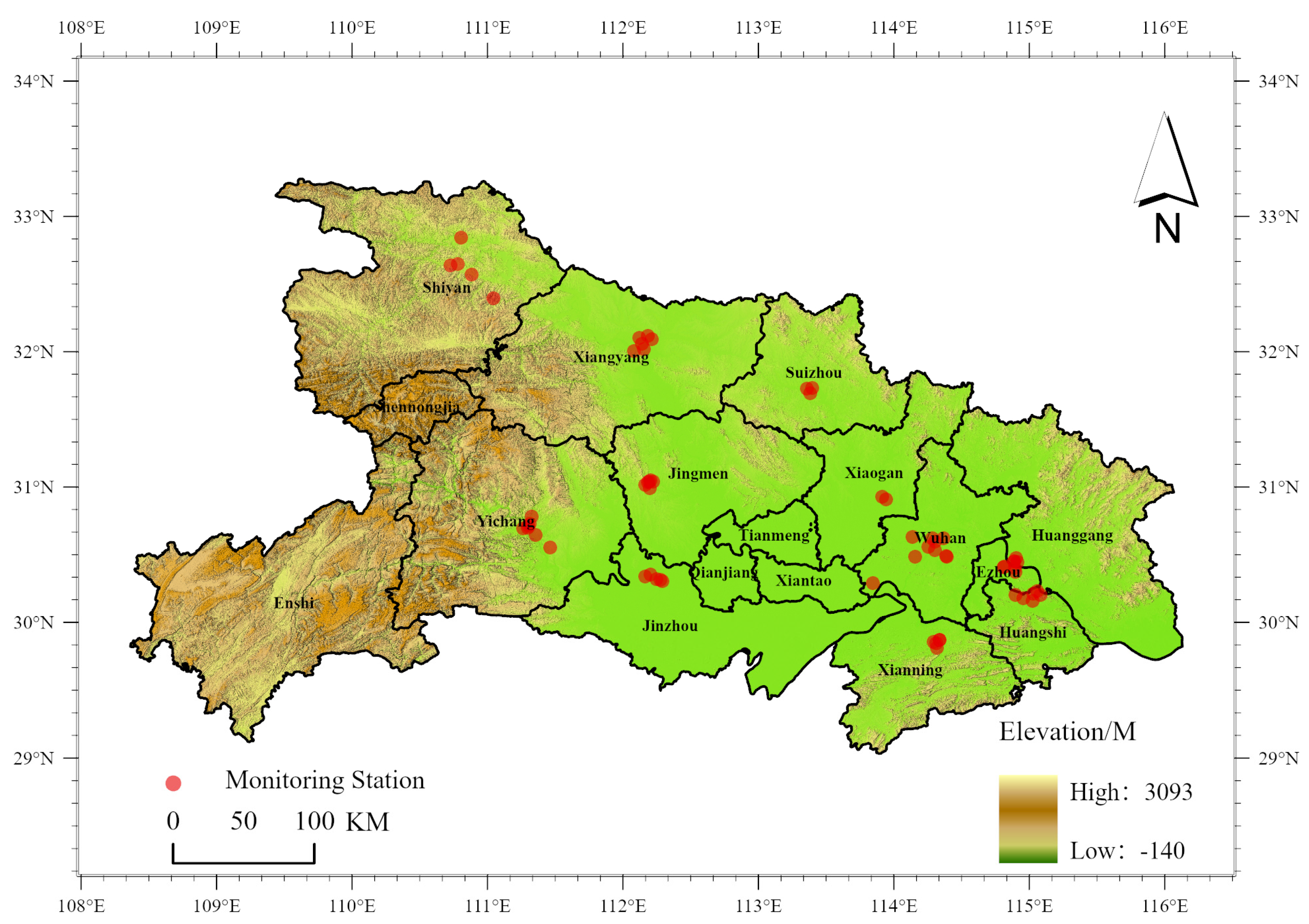
2.1. Study Area

This study took Hubei Province as the research area. Hubei Province is located in the middle of China, with a geographical range of approximately 29° to 33° north latitude and 110° to 116° east longitude, with a total area of about 185,900 square kilometers. This area has complex and diverse landforms, including plains, hills, and mountains, and is an important part of the middle reaches of the Yangtze River Economic Belt, with rich natural resources and a relatively complete industrial base. These characteristics make Hubei Province an ideal region to explore the spatial and temporal distribution of urban and regional air quality and ozone pollution. In consideration of research requirements and data availability, 63 representative ground monitoring stations (see Figure 1) in Hubei Province were selected for this study. These stations were evenly distributed in major cities such as Wuhan, Xiangyang, Yichang, and Huangshi, and their surrounding areas, covering 12 prefecture-level cities in the province, so as to reflect regional air quality characteristics in a more comprehensive way. It provides a solid database for the in-depth analysis of the temporal and spatial distribution of near-surface ozone pollution in Hubei Province.

2.2. Technology Roadmap

This study proposes a comprehensive framework for the estimation of near-surface ozone concentrations in Hubei Province by integrating multisource data, including natural environmental variables, satellite-based remote sensing observations, and anthropogenic activity indicators (Figure 2). All data were standardized in terms of format, spatial reference system, and spatiotemporal resolution to ensure consistency and comparability. Ground-based ozone measurements were paired with corresponding predictor variables to construct training samples. A suite of machine learning algorithms—namely XGBoost, LightGBM, and CatBoost—were employed for model development, followed by model selection, ensemble learning, and validation. The proposed approach enables accurate and spatially refined estimation of surface-level ozone concentrations, providing methodological support for regional air quality assessment and management.

2.3. Data and Preprocessing

2.3.1. Data Overview

The ozone station monitoring data came from China’s air quality historical data released by the China General Environmental Monitoring Station (CNEMC). This dataset provides detailed 1 h mean ozone monitoring records, covering long-term observation data of multiple monitoring stations, with a high temporal resolution and reliability, as shown in

Table 1. Sources, spatial resolutions, and temporal resolutions of datasets used in this study. Abbreviations are explained below.

Name	Time Resolution	Spatial Resolution	Source
O3	——	1 h	CNEMC
TRO_O3	1113.2 m	1 d	GEE
TRO_NO2	1113.2 m	1 d	GEE
D2M	0.5° × 0.5°	1 d	ECMWF
T2M	0.5° × 0.5°	1 d	ECMWF
Lai_hv	0.5° × 0.5°	1 d	ECMWF
Lai_lv	0.5° × 0.5°	1 d	ECMWF
SP	0.5° × 0.5°	1 d	ECMWF
SSR	0.5° × 0.5°	1 d	ECMWF
STR	0.5° × 0.5°	1 d	ECMWF
TP	0.5° × 0.5°	1 d	ECMWF
U10	0.5° × 0.5°	1 d	ECMWF
V10	0.5° × 0.5°	1 d	ECMWF
BLR	0.5° × 0.5°	1 d	ECMWF
BLH	0.5° × 0.5°	1 d	ECMWF
POP_LIGHT Road	500 m ——	1 m 1 y	GEE OSM

CNEMC: China National Environmental Monitoring Center; GEE: Google Earth Engine; ECMWF: European Centre for Medium-Range Weather Forecasts; OSM: OpenStreetMap; O₃: ground-level ozone concentration; TRO_O₃: tropospheric ozone column concentration; TRO_NO₂: tropospheric nitrogen dioxide column concentration; D2M: 2 m dew point temperature; T2M: 2 m air temperature; Lai_hv: leaf area index of high vegetation; Lai_lv: leaf area index of low vegetation; SP: surface pressure; SSR: surface solar radiation (downward); STR: surface thermal radiation (downward); TP: total precipitation; U10/V10: 10 m zonal/meridional wind speed; BLR: boundary layer relative humidity; BLH: boundary layer height; POP_LIGHT: nighttime light-based population proxy; road: road network density or vector data.

.

2.3.2. Satellite Ozone Data

The Sentinel-5P/TROPOMI Near Real-Time (NRTI) L3 atmospheric composition product of the Google Earth Engine (GEE) platform was adopted in this study (Table 1). Based on the grid-based dataset generated by L2 data inversion, two parameters were selected: the NO₂ column concentration and the O₃ column concentration. The former was used as an ozone precursor to characterize the driving mechanism of photochemical reactions, and the latter to analyze the spatiotemporal differentiation of ozone and its variation rules. The data were preprocessed by cloud mask and radiation correction, which effectively reduced the uncertainty of inversion.

2.3.3. Meteorological Data

Meteorological conditions exert a significant influence on the formation, deposition, and transport of tropospheric ozone. As a typical secondary pollutant formed through photochemical reactions, near-surface ozone is primarily produced via the interaction of ultraviolet (UV) radiation with its precursors, notably nitrogen oxides (NO_x) and volatile organic compounds (VOCs). While meteorological variables such as temperature and relative humidity may modulate reaction kinetics, they do not directly control the photochemical production of ozone (European Environment Agency) [16].

Water vapor, as a key atmospheric constituent, may indirectly affect ozone formation by altering cloud formation and coverage. Increased water vapor enhances cloud optical thickness, thereby attenuating UV radiation reaching the surface and reducing the efficiency of photochemical ozone production (Photochemical & Photobiological Sciences, 2015) [17]. However, these interactions are complex, nonlinear, and often regionally dependent, thus requiring careful interpretation and further empirical validation.

The role of vegetation, particularly the leaf area index (LAI), is more directly associated with ozone deposition rather than its formation. The LAI regulates dry deposition processes by modifying aerodynamic and surface resistance and by influencing the stomatal uptake of ozone by vegetation. Consequently, changes in the LAI can significantly impact surface ozone concentrations through enhanced or suppressed deposition (Zhou et al., 2018) [18]. Additionally, the LAI can influence regional energy and moisture fluxes via evapotranspiration, potentially affecting boundary layer development and pollutant dispersion; nonetheless, such feedbacks remain secondary and context-specific [19].

2.3.4. Human Activity Data

Human activity data, such as population distribution and traffic conditions, play an important role in ozone generation by influencing O₃ precursor emissions, such as nitrogen oxides (NO_x) and volatile organic compounds (VOCs). Among them, high-population-density areas are usually accompanied by higher energy consumption and industrial emissions, while dense road networks become one of the main sources of ozone precursors due to vehicle exhaust emissions, which can contribute to elevated ozone levels under favorable photochemical and meteorological conditions.

This study used the Visible Infrared Imaging Radiometer Suite (VIIRS) night light data (since 2018) provided by the Google Earth Engine (GEE) platform to characterize the effect of population activity on near-surface ozone concentrations. In addition, in order to explore the role of traffic factors in ozone pollution, the road network data from 2018 to 2023 provided by the OpenStreetMap (OSM) platform was obtained and used for subsequent quantitative analysis. The details of the relevant data are shown in Table 1.

2.3.5. Data Preprocessing

In this study, the latitude and longitude information of each monitoring station in Hubei Province was first sorted out, and based on this information, the meteorological parameters of corresponding locations were extracted from the meteorological grid data, and the average daily ozone concentration of each station was calculated. Considering the differences in the spatial and temporal resolution of the original data, in order to ensure data consistency and comparability, cubic interpolation was used in this study to resample the meteorological data, adjust them uniformly to a spatial resolution of 0.01° × 0.01°, and convert them into daily scale data. In addition, in order to achieve accurate spatiotemporal matching, all datasets were uniformly used in the WGS84 coordinate system.

In terms of road data processing, the original road data were stored as vector line features. To construct a spatially consistent road network density index, the study area was divided into fixed grids of 0.01° × 0.01°, within which the total road length was calculated. This index reflects the spatial heterogeneity of road infrastructure and serves as a proxy indicator of potential traffic activity and vehicle emissions, especially in the absence of direct traffic flow data. It, thus, provides a quantitative basis for analyzing the possible impact of road-related emissions on ozone concentrations.

2.4. Methods

2.4.1. Basic Machine Learning Model

In this study, the performance of six machine learning algorithms in ozone concentration estimation was systematically evaluated, and the models with a better estimation performance were selected for the construction of integrated models to improve the accuracy of near-surface ozone estimation. The core advantages of each model and its correlation with the ozone generation mechanism were as follows:

(1)

Classification and regression tree (CART)

It generates interpretable decision rules based on recursive dichotomies and is good at identifying threshold effects of ozone drivers. However, its single-tree structure is sensitive to monitoring noise and needs to be integrated to improve its stability.

(2)

CatBoost

The symmetrical tree structure can effectively capture the complex interaction between ozone precursors and meteorological factors by using the orderly lifting strategy to avoid gradient leakage risk.

(3)

Extreme Trees (EXT)

The random splitting strategy is used to enhance model diversity, and its randomization characteristics can alleviate the feature importance bias caused by spatial matching errors and show stronger generalization ability in the ozone spatial heterogeneity region.

(4)

XGBoost

Second-order optimization and regularization constraints are introduced to improve the prediction accuracy. The sparse-sensing mechanism can automatically deal with missing values in ozone monitoring data.

(5)

Random Forest (RF)

The dual randomization strategy (sample/feature) avoids the dependence on a single strong correlation factor, and the multi-tree-voting mechanism effectively alleviates local overfitting in complex terrain.

(6)

LightGBM (LGBM)

The histogram algorithm accelerates large-scale data training, and the leaf-wise growth strategy can accurately characterize the difference in the ozone concentration gradient between urban agglomeration and the natural interval.

2.4.2. Integrated Methods

Based on the performance evaluation results of the above six single models, several models with a good fitting effect and high R² were selected to construct an integration framework. In this study, two integration frameworks were constructed and compared, and the integration method with the better integration fitting effect was selected as the final integration scheme. The integration methods are as follows:

(1)

Voting Integration

The voting method integrates the estimation results of different base models through majority voting and uses the complementarity of the errors of each model to balance the differences in the characterization of ozone generation and diffusion in different temporal and spatial environments so as to reduce the overfitting risk of a single model, improve the tolerance of data noise and matching errors, and enhance the robustness of the overall model.

(2)

Stacking Integration

The stacking method adopts the two-level modeling strategy, which selects several single models with the best fitting effect in the primary layer and takes their estimated output as the input of the secondary model. The secondary layer uses ridge regression to integrate the output of the primary model, solves the multicollinearity problem with L2 regularization constraints, and ensures that the training data of the secondary model are completely independent of the primary model training set (using 20% samples that were not involved in the primary training in the 50-fold cross-validation) so as to improve the model’s generalization ability. This method can fully balance the difference in ozone generation and diffusion mechanisms in different regions (such as urban agglomeration and remote regions) and different seasonal conditions and, thus, significantly improve the overall estimation performance.

2.4.3. Feature Selection

(1)

Feature correlation analysis

Based on the complexity of the ozone generation mechanism, the Pearson correlation coefficient was used to quantify the linear correlation between input variables and near-surface ozone concentrations. The analysis focused on the potential effects of ozone precursors (e.g., NO₂), meteorological factors (e.g., T2M, SSR, and BLH), and human activity indicators (e.g., road density) on ozone concentrations. By screening significantly related features as input variables to the model, the interference of redundant information was effectively reduced, while the photochemical and transmission process information of key driving factors was retained, providing a scientific basis for subsequent modeling.

(2)

Characteristic ablation experiment

Before model training, all variables in the sample were taken as independent variables, and then the model was asked to make multiple rounds of estimation, and one variable was eliminated one by one in each round. The order of variable elimination was arranged from small to large according to its correlation with the target variable (the true value of the near-surface ozone concentration), until only one variable remained in the estimation model. The evaluation indicators R2, RMSE, SLOPE, and intercept of each round of the model estimation effect were recorded, and a line chart was plotted. The contribution and sensitivity of each variable to the model effect were intuitively understood by observing the changes in the indicators, and variables with a low contribution and sensitivity were eliminated so that the model could focus on the most valuable variables for estimation. Thus, the estimation accuracy and stability of the model could be improved, and overfitting problems caused by excessive noise information could be avoided.

2.4.4. Model Evaluation

In this study, the performance of each model was evaluated by the method of 50-fold cross-validation. For the base model, the evaluation criteria included the root-mean-square error (RMSE), coefficient of determination (R²), regression slope, and intercept. Among them, a low RMSE, an R² approaching 1, a regression slope approaching 1, and an intercept approaching 0 all suggested that the model had a high estimation accuracy.

In order to further reveal the linear relationship between the estimated value and the actual value, this study introduced the evaluation index of the regression slope and intercept and fitted the linear relationship between the estimated value and the actual value through the least-squares method. The regression slope was defined as

$$\mathrm{Slope} = {\displaystyle \frac{{\sum }_{i=1}^n \left(\widehat{y_i} - \overline{\widehat{y}}\right)\left(y_i - \overline{y}\right)}{{\sum }_{i=1}^n {\left(\widehat{y_i} - \overline{\widehat{y}}\right)}^2}}$$

The intercept was calculated as

$$\mathrm{Intercept}=\overline{y}-\mathrm{Slope}\times \overline{\widehat{y}}$$

where $y_i$ and $\widehat{y_i}$ are the actual values and estimated values, respectively, and $\overline{y}$ and $\overline{\widehat{y}}$ are their corresponding mean values. Ideally, if the model estimates are perfect, the slope should be close to 1, and the intercept should be close to 0.

For the integrated model, the average absolute error (MAE), relative error (R_value), and correlation coefficient (R_value) indexes were further introduced on the basis of the above so as to more comprehensively quantify the error level, error proportion, and correlation between the predicted results and the actual value.

3. Results

3.1. Results of Model Evaluation

3.1.1. Basic Model Comparison

Based on the constructed high-quality training sample set, this study systematically screened six mainstream machine learning algorithms for modeling analysis. These included classification and regression trees (CART), Extra-Trees (EXT), random forest (RF), XGBoost, LightGBM, and CatBoost to systematically evaluate the predictive performance of the different algorithms. In order to ensure the rigor of model validation, five-fold cross-validation was used to evaluate the robustness of the model performance. Through systematic comparison and analysis, the performance of each algorithm in terms of key evaluation indicators is shown in Figure 3.

Figure 3 presents a comparative evaluation of the six machine learning models based on the coefficient of determination (R²) and mean absolute error (MAE). Among them, LightGBM achieved the highest performance (R² = 0.87; MAE = 8.06), explaining 87% of the variance in the target variable and reducing the prediction error by 13.0% relative to the second-best model. This result highlights its strong capability to capture complex nonlinear relationships and generalize across heterogeneous data. XGBoost ranked second (R² = 0.83; MAE = 9.26), offering a good balance between accuracy and computational efficiency through regularization and parallel processing. CatBoost also performed competitively (R² = 0.82; MAE = 9.62), exhibiting particular advantages in handling categorical features via ordered boosting and automatic encoding. In contrast, traditional decision-tree-based models showed notably weaker predictive power. CART (R² = 0.62; MAE = 14.0) was limited by its inability to model high-dimensional nonlinear patterns, while EXT (R² = 0.76; MAE = 11.17) and RF (R² = 0.75; MAE = 11.37) partially mitigated overfitting through ensemble strategies but remained inferior in residual learning and overall accuracy. In summary, LightGBM, XGBoost, and CatBoost—representing state-of-the-art gradient-boosting models—demonstrated a superior predictive accuracy and generalization capability, making them well-suited for constructing a robust evaluation framework for kilometer-scale near-surface ozone concentration inversion.

3.1.2. Analysis and Selection of Characteristic Variables

The data sources of this study included meteorological data, TROPOMI satellite observation data, and night light data. Before the model was constructed, the following feature variables were screened by calculating the feature correlation.

Meteorological variables, such as temperature, relative humidity, boundary layer height, wind speed, etc., directly affect the formation and diffusion process of ozone.

Atmospheric composition variables, such as NO₂ and O₃ concentrations, are key catalysts for photochemical reactions.

The road network density reflects the intensity of human activities and is related to the level of pollutant emissions.

In data preprocessing, the missing values were eliminated, interpolation was completed, and the data source was aligned in time and space to ensure the consistency of the input data. After statistical analysis, the correlation between ozone and characteristic variables was obtained, as shown in Figure 4.

Based on the Pearson correlation coefficient distribution of each characteristic variable and near-surface ozone concentration in Figure 4, the correlation mechanism and environmental impact could be systematically analyzed. The SSR (r = 0.6) and T2M (r = 0.6), as the dominant factors, had significant positive effects on ozone generation: Solar radiation provides the necessary energy for the photochemical reaction and directly drives the photolysis reaction between NO_x and VOCs [20], while the high-temperature environment further enhances ozone production by accelerating the reaction kinetic rate (Arrhenius effect) [21] and promoting the volatilization release of precursors (such as VOCs) [22]. Although the elevation of BLH (r = 0.4) may enhance the vertical velocity [23], the net effect tends to extend the photochemical reaction time under the synergistic effect of strong radiation and high temperature [18]. The positive correlation of D2M (r = 0.4) may be due to its strong coupling with surface temperature (ECMWF homology data), which masks the potential inhibitory effect of humidity on ozone generation [24]. The low LAI_LV (r = 0.4) exerts dual indirect influences on ozone levels: (1) suppressing the dry deposition removal capacity [25] and (2) potentially enhancing biological VOC emissions during peak seasons [18]. Notably, TRO_NO₂ (r = −0.3) displays a significant negative correlation with ozone concentrations, demonstrating the characteristic NO_x titration mechanism in photochemical cycles. This phenomenon occurs where excess NO₂ suppresses net ozone production through two pathways: radical scavenging (e.g., OH consumption) and direct ozone destruction via the NO + O₃ → NO₂ + O₂ reaction [26].

Figure 5 shows the results of XGBoost, LightGBM, and CatBoost passing the above tests (A_O and R_D represent the tropomi ozone concentration and road network density, respectively). The results show when the features strongly related to the ozone concentration (such as the leaf area index (high) and surface net thermal radiation) were excluded, the R² values of the three models decreased significantly, and the RMSE increased significantly, indicating that such variables had a significant effect on the explanatory power of the models. For example, in the figure below, after the removal of u10 and sp, the R² of the three models decreased significantly. This is consistent with the correlation coefficients of u10 and sp in the figure above (both close to 0.2). In addition, after the removal of some variables (such as the 2 m leak point temperature), the model performance fluctuated slightly (R² change < 0.05; RMSE increase < 5 μg/m³), and the slope and intercept remained stable, indicating limited contribution or noise interference. There were also differences between the models: it can be seen from the figure that XGBoost had the highest sensitivity to features, and RMSE presented a step increase with variable elimination. However, CatBoost was more robust to some missing or distorted variables (such as a low leaf area index) due to the built-in feature-processing mechanism. The final results show that the selected feature variables were strongly correlated with ozone, and the ablation of any feature led to a reduction in model accuracy, so this paper chose to use all initial variables for subsequent training and estimation.

3.1.3. Integration Model Selection

After the optimization of the model integration strategy, each evaluation index presented a systematic improvement. The determination coefficient (R²) of the integrated model based on Stacking was 0.895, which was 2.87% higher than the LightGBM individual model with the best performance in the baseline model. The integrated model R² based on voting was 0.894, corresponding to a 2.76% increase. Error analysis showed that the mean absolute error (MAE) of the integrated model was 14.76% and 14.01% lower than that of the benchmark model, respectively, which verified the improvement effect of the integrated method on the prediction accuracy.

The integrated framework constructed in this study combined the modeling advantages of three gradient lifting models (XGBoost, LightGBM, and CatBoost) through differentiation strategies: The stacking method used a meta-learner to dynamically weight the integrated base model to predict the distribution, and the voting rule coordinated the output of multiple models based on a consensus mechanism. As shown in Figure 6, the two schemes achieved a performance jump by reducing the synergistic effect of prediction variance and bias while retaining the ability to interpret the features of the base model. The performance gains resulted from the complementarity of features among heterogeneous models and the balanced optimization of the error distribution by the integrated strategy, resulting in a more stable prediction distribution and better generalization ability.

For the two integrated models, the stacking method and the voting method, although the determination coefficients of the two models for sample estimation were similar (0.91 and 0.90), the relative error of the stacking method-integrated model was significantly lower than that of the voting method-integrated model. The mean relative error of the voting-integrated model reached 12.08165%, while that of the stacking-integrated model was only 10.74244%. Moreover, the MAE of the stacking-integrated model was 4.87% lower than that of the voting-integrated model, showing better performance. Therefore, the optimal integration strategy (stack method) was selected for the final model estimation.

In summary, the XGBoost, LightGBM, and CatBoost models were selected as the base model, and all initial characteristic variables were used for model training. After model integration using the stacking method, the final near-surface ozone estimation was performed.

3.2. Spatial Heterogeneity of Ozone Distribution

Based on the integrated model, we conducted daily estimates of the near-surface ozone concentrations for Hubei Province from October 2018 to December 2023 and processed the results into annual, quarterly, and other time scales.

3.2.1. Annual Ozone Distribution

Figure 7 shows the annual mean ozone distribution in Hubei Province. From the perspective of a single year, it is generally the case that the annual mean of the near-surface ozone concentration in the eastern part of Hubei Province is higher than that in the western part, especially in the area around Wuhan. Taking 2019 as an example, the annual mean value of near-surface ozone in cities such as Wuhan (79 μg/m³), Suizhou (81 μg/m³), Xiaogan (77 μg/m³), and Xiantao (77 μg/m³) in the east was greater than that in parts of the Enshi Tujia and Miao Autonomous Prefecture (76 μg/m³) and Yichang (72 μg/m³) in the west. According to the figure, there is basically a dividing line connecting the western curve of Shiyan City to the southern part of Jingzhou City. Near-surface ozone concentrations were lower west of the boundary line and significantly higher east of it. The formation mechanism of this spatial pattern is mainly affected by multiple factors: First, there are significant differences in topographic dynamics. The eastern Jianghan Plain is low and flat (average altitude < 50 m), and the atmospheric boundary layer is relatively stable, which inhibits the diffusion of pollutants [27], while the western mountainous region (average altitude > 800 m) promotes the vertical transport of ozone preformed through enhanced turbulent mixing [28]. Second, the anthropogenic emission intensity is significantly different. According to the Multi-Resolution Emission Inventory for China (MEIC), the emission intensities of VOCs and NO_x in the eastern industrial agglomeration region—primarily dominated by iron and steel and chemical industries—are estimated to be 4.2 and 3.7 times greater, respectively, than those in the western region [29]. Such elevated precursor emissions contribute significantly to the photochemical formation of ozone. Third, the high vegetation coverage rate (>60%) in the west can reduce the surface ozone concentration by 10–15% through stomatal absorption and dry sedimentation [30], while the ozone reduction efficiency of the eastern farmland ecosystem is only 1/3 of that of the forest [31]. Fourth, the average annual temperature (16.5–17.2 °C) and sunshine duration (1850–1950 h) in the east are 1.8 °C and 200 h higher than those in the west, significantly increasing the photochemical reaction rate [32]. The synergistic effects of the above factors together shape the east–west differentiation pattern of the ozone concentration.

Looking at the annual average for the five years from 2019 to 2023, there was also a difference. For example, the peak in 2019 reached 70 μg/m³, and the near-surface ozone value was at a high level. The annual average for 2020 was only 67 μg/m³, and ozone levels in all parts were lower than in 2019, especially in the eastern region. This was mainly due to the outbreak of the novel coronavirus pneumonia at the end of 2019, which led to the lockdown of Wuhan and a period of epidemic prevention and control across the country. Industrial production was significantly reduced, domestic and industrial emissions were reduced, and the formation of ozone precursors such as NO₂ and HCHO was significantly reduced, delaying the occurrence of ozone photochemical reactions. The near-surface O₃ in 2020 and 2021 was located at a low level. With the resumption of production, emissions from production activities gradually increased, and the ozone concentration increased in 2022 and 2023, reaching a maximum of 75 μg/m³ and 71 μg/m³, respectively.

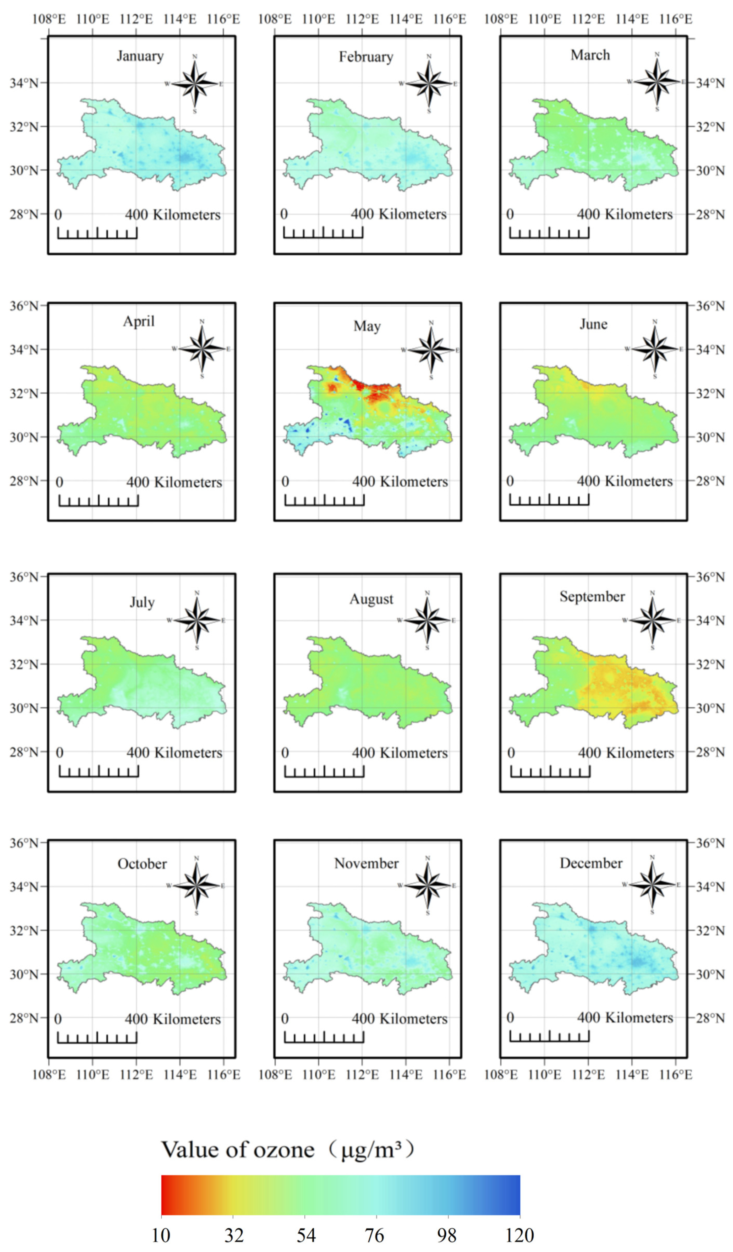
3.2.2. Quarterly and Monthly Ozone Distribution

The quarterly distribution of ground-level ozone from 2019 to 2023 is presented in Figure 8.

Based on an optimized integrated model, we estimated the near-surface ozone concentrations for each quarter from 2019 to 2020. Overall, the ozone concentration in the first quarter was generally at a low level, the average ozone concentration was only 65 mu g/m³, the ozone concentration in the second quarter was significantly increased, that in the third quarter was decreased compared with the second quarter, and that in the fourth quarter was basically the same as in the first quarter.

In theory, near-surface ozone concentrations should be highest in summer, followed by autumn, and lower in winter and spring. The high concentration of near-surface ozone in summer is mainly driven by the enhancement of photochemical reactions and the accumulation of precursors. Strong ultraviolet radiation and high temperature significantly accelerate the photochemical cycle of nitrogen oxides (NO_x) and volatile organic compounds (VOCs), in which NO₂ photolysis occurs under ultraviolet light to form reactive oxygen atoms (O), which are combined with O₂ to form ozone (O₃). However, from the results, the ozone concentration in the second quarter was the highest. The second quarter was in April, May, and June, the third quarter was in July, August, and September, and the summer was in June, July, and August, and the convergence with the third quarter was higher. This result is different from the conclusion that the ozone concentration is generally high in summer.

In order to deeply explore the reason why the second quarter of Hubei Province was the quarter with the highest ozone concentration in the whole year, we estimated the monthly average near-surface ozone concentration from 2019 to 2023 based on the final integrated model, and the results are shown in Figure 9.

From an overall perspective, the spatial distribution of surface ozone in Hubei Province shows a pattern of higher concentrations in the east and lower in the west. September stands out as the month with the highest annual ozone concentrations, with some regions reaching up to 100 μg/m³. This is followed by May, April, and June. Notably, ozone levels in July and August were relatively lower, which aligned with the earlier analysis showing peak concentrations in the second quarter of the year. At the site level, the number of stations recording ozone concentrations above 85 μg/m³ in the second quarter (April–June) from 2019 to 2023 exceeded that in the third quarter, further confirming that surface ozone levels in Hubei Province were significantly higher in Q2 than in Q3.

This seasonal variation can be attributed to multiple factors. From the perspective of human activities, elevated ozone concentrations in Q2 are closely related to intensive agricultural emissions and regional meteorological conditions. According to the National Remote Sensing Monitoring Report on Straw Burning [33], straw-burning activities in Hubei Province are predominantly observed from April to June, coinciding with the wheat and early rice harvest season. This period is characterized by significant emissions of volatile organic compounds (VOCs) and nitrogen oxides (NO_x)—key precursors of ozone formation—released during biomass burning. Straw burning, as noted by Zhu et al. [34], substantially deteriorates air quality, while the emissions of formaldehyde, acetaldehyde, benzene, and toluene contribute significantly to the ozone formation potential (OFP). These emission patterns and photochemical mechanisms are consistent with those observed in other major agricultural zones in China.

Meteorological conditions in late spring and early summer—including elevated temperatures, strong solar radiation, and stagnant air masses—create favorable conditions for ozone formation by accelerating photochemical reactions. Tian et al. [35] observed that such conditions are associated with intensified ozone pollution in Central China, posing elevated risks to human health. Moreover, temperature inversion layers during these periods reduce the atmospheric mixing height, prolonging the residence time of ozone and its precursors. Mbululo et al. [36] similarly found that ozone pollution episodes in Wuhan often coincided with boundary layer stagnation, weak winds, and low turbulence, all of which contributed to ozone accumulation.

However, drought conditions introduce further complexity. As highlighted by Juráň et al., drought can suppress the primary ozone sink—vegetation—by inducing stomatal closure to conserve water, thereby reducing stomatal ozone flux [37]. This physiological response not only diminishes ozone uptake but also exacerbates ozone accumulation in the atmosphere. Simultaneously, high radiation and low humidity under drought further enhance ozone production while limiting its deposition. Although non-stomatal pathways (e.g., cuticular and soil deposition) may partially compensate, the overall sink capacity is generally weakened. Therefore, drought not only promotes ozone formation through enhanced photochemical conditions but also inhibits removal processes, ultimately leading to a compounding effect on ozone pollution during dry and sunny periods. Additionally, the nonlinear relationship between ozone production and the VOCs/NO_x ratio explains the seasonal differences. Mao et al. [38] demonstrated that when the VOCs/NO_x ratio exceeds 8:1—typical during biomass burning—ozone formation enters a VOC-sensitive regime, and production increases sharply with higher precursor concentrations. In contrast, summer traffic emissions tend to elevate NO_x levels, shifting the system toward a NO_x-sensitive or even titration-limited regime, which suppresses ozone formation.

4. Discussions

This study developed a high-resolution framework for estimating near-surface ozone by integrating multi-source datasets with ensemble machine learning techniques. Compared with conventional approaches, this model demonstrates substantial improvements in predictive performance, achieving an R² of 0.91 and an RMSE of 9.40 μg/m³. While these statistical metrics confirm the model’s effectiveness, a deeper examination of its underlying mechanisms and broader implications is warranted.

Spatiotemporal analysis revealed a distinct east–west gradient in ozone distribution, with elevated concentrations observed in the industrialized eastern plains (e.g., Wuhan), and lower concentrations in the mountainous western regions (e.g., Enshi). This spatial pattern reflects the combined influence of anthropogenic emissions, topographic constraints, and vegetation-mediated ozone deposition. In eastern urban clusters, intensive industrial and vehicular activities contribute high levels of NO_x and VOCs, while flat terrain and stable boundary layers inhibit vertical pollutant dispersion. Conversely, the western region benefits from extensive vegetation cover (LAI > 60%), which enhances the dry deposition of ozone, and from the complex mountainous topography that promotes turbulent mixing. These findings are consistent with prior studies conducted in the Yangtze River Delta, where emission–topography interactions have been identified as key drivers of ozone heterogeneity [39].

A notable seasonal anomaly was also identified: ozone concentrations peaked during the second quarter (April–June) rather than the typical midsummer months (July–August), with September exhibiting the highest monthly averages. This deviation from the expected seasonal pattern may be explained by two main factors. First, intensified agricultural activities, such as straw burning in late spring, significantly increase VOC emissions, which possess a high ozone formation potential (OFP), as evidenced by emission inventory studies [35]. Second, the meteorological conditions prevalent in April to June—characterized by high temperatures (>30 °C), strong solar radiation, and frequent temperature inversions—create an optimal environment for photochemical ozone formation while simultaneously suppressing vertical dispersion [37]. The observed summertime trough may be further explained by increased NO_x emissions from vehicles, which can push the atmospheric chemistry into a NO_x-saturated regime. In such a regime, as described by Jacob and Winner (2009) [31], additional NO_x can actually suppress ozone formation by titrating ozone or altering the balance of photochemical reactions, particularly under intense solar radiation and stagnant meteorological conditions.

To reduce the risk of overfitting, this study employed a stacked ensemble learning approach that combined structurally diverse gradient-boosting algorithms—XGBoost, LightGBM, and CatBoost—with a meta-learning strategy. This architecture leveraged the strengths of each base learner while mitigating their individual weaknesses. Compared with previous studies that primarily relied on single learners or conventional ensemble models, our method provides greater robustness and generalization, particularly under spatial heterogeneity. For instance, Fan et al. (2023) applied a two-stage random forest model with cross-validation to constrain overfitting, but lacked structural diversity across models and did not incorporate hysteresis features, which are essential for capturing temporal ozone dynamics [40].

Our study also emphasizes the interpretability and mechanistic relevance of selected features. Through systematic feature ablation experiments, we confirmed the critical contributions of variables such as LAI, solar radiation, and boundary layer height. The performance deterioration observed after their removal (e.g., R² decrease > 0.1; RMSE increase > 5 μg/m³) aligns well with their known roles in ozone chemistry and deposition. In contrast, Zhang et al. (2022) proposed a BO-XGBoost-RFE feature selection framework that emphasizes predictive performance but gives limited attention to the atmospheric or photochemical relevance of the selected variables [41]. By integrating both statistical and physical reasoning into the feature selection process, our model not only improves accuracy but also enhances scientific transparency and interpretability.

Despite the promising performance of the model, several limitations should be acknowledged. One key limitation concerns the representation of human activity: proxy variables such as nightlight data may fail to reflect real-time emission dynamics, particularly in rapidly developing urban areas. Additionally, the model relies on externally prescribed meteorological inputs and lacks dynamic coupling between vegetation and the atmosphere. This restricts the model’s ability to simulate biogeochemical feedbacks that are critical to understanding ozone–vegetation interactions. Moreover, stomatal-level ozone uptake—an important physiological mechanism through which vegetation modulates ozone deposition and feedback strength—is not explicitly accounted for. Future research should consider integrating high-temporal-resolution emission inventories, implementing coupled land–atmosphere modeling frameworks, and applying the model in data-sparse or topographically complex regions. These advancements will be essential for enhancing both the predictive accuracy and the process-level realism of ozone estimation frameworks.

5. Conclusions

This study developed a high-resolution near-surface ozone estimation model for Hubei Province (2018–2023) by integrating multiple machine learning algorithms to overcome the limitations of traditional models’ insufficient resolution and single-model overfitting issues. The optimized ensemble model achieved exceptional performance with an overall R² of 0.91, RMSE of 9.40 μg/m³, and MAE of 6.44 μg/m³ at a 1 km spatial resolution. Spatial analysis revealed a distinct east–west gradient, with elevated ozone concentrations around the Wuhan metropolitan area and lower levels in the western Enshi Prefecture. Temporally, annual variations showed relatively higher ozone levels in 2019, 2022, and 2023, contrasting with reduced concentrations during the 2020–2021 pandemic containment periods. Seasonal patterns demonstrated peak concentrations in the second quarter (April–June), followed by the third quarter (July–September), with the lowest levels occurring in the winter and early spring quarters (Q1 and Q4). Monthly variations exhibited a primary peak in September, secondary peaks from April to June, and sustained low concentrations during November–February. Notably, an atypical summer trough was observed in June–July, potentially associated with regional meteorological conditions or pollution control measures, warranting further investigation.

References

1. Zhang, J.; Wei, Y.; Fang, Z. Ozone Pollution: A Major Health Hazard Worldwide. Front. Immunol. 2019, 10, 2518. [Google Scholar] [CrossRef]
2. Fan, B.; Wang, W.; Geng, C.; Xu, B.; Song, Z.; Liu, Y.; Yang, W. Composition of Photochemical Consumed Volatile Organic Compounds and Their Impact on Ozone Formation Regime: A Case Study in Zibo, China. Atmos. Environ. 2025, 343, 120984. [Google Scholar] [CrossRef]
3. Zhang, M.; Liu, Y.; Xu, X.; He, J.; Ji, D.; Qu, K.; Xu, Y.; Cong, C.; Wang, Y. A Systematic Review on Atmospheric Ozone Pollution in a Typical Peninsula Region of North China: Formation Mechanism, Spatiotemporal Distribution, Source Apportionment, and Health and Ecological Effects. Curr. Pollut. Rep. 2025, 11, 9. [Google Scholar] [CrossRef]
4. Du, N.; Chen, L.; Liao, H.; Zhu, J.; Li, K. Impact of Summer Tropospheric Ozone Radiative Forcing on Meteorology and Air Quality in North China. Environ. Sci. 2023, 44, 3705–3714. Available online: https://www.hjkx.ac.cn/hjkx/ch/html/20230709.htm (accessed on 11 March 2025).
5. Xie, X.-D.; Hu, J.-L.; Zhang, Y.-H. Research Topic and Trend Analysis of Ozone Pollution in China Based on Bibliometric Review. Chin. Environ. Sci. 2024, 44, 6513–6521. [Google Scholar] [CrossRef]
6. Department of Ecology and Environment of Hubei Province (DEEHP). Annual Report on Air Quality in Hubei Province; Hubei Provincial Department of Ecology and Environment: Wuhan, China, 2020. Available online: https://sthjt.hubei.gov.cn (accessed on 15 June 2024).
7. Zong, M.; Song, T.; Zhang, Y.; Feng, Y.; Fan, S. A Deep Forest Algorithm Based on TropOMI Satellite Data to Estimate Near-Ground Ozone Concentration. Atmosphere 2024, 15, 1020. [Google Scholar] [CrossRef]
8. Yang, Z.; Li, Z.; Cheng, F.; Lv, Q.; Li, K.; Zhang, T.; Zhou, Y.; Zhao, B.; Xue, W.; Wei, J. Two-Decade Surface Ozone (O3) Pollution in China: Enhanced Fine-Scale Estimations and Environmental Health Implications. Remote Sens. Environ. 2024, 317, 114459. [Google Scholar] [CrossRef]
9. Huang, K.; Luo, W.; Wan, C.; Gong, M.; Ma, J. Estimation of Near-Surface Ozone Concentrations in China from 2001 to 2020. J. Atmos. Environ. Opt. 2024, 19, 646. [Google Scholar] [CrossRef]
10. Xia, N.; Li, A.; Quan, W.; Tang, M.; Tang, Y.; Xu, Z. Analysis of Ground-Level Ozone Pollution and Its Driving Factors Based on GTWR in China. Trans. Chin. Soc. Agric. Eng. 2024, 40, 283–293. [Google Scholar] [CrossRef]
11. Gong, D.; Du, N.; Wang, L.; Zhang, X.; Li, L.; Zhang, H. Estimation of Near-Surface Ozone Concentration in the Beijing-Tianjin-Hebei Region Based on XGBoost-LME Model. Environ. Sci. 2024, 45, 3815–3827. [Google Scholar] [CrossRef]
12. Song, S.P.; Fan, M.; Tao, J.H.; Chen, S.M.; Gu, J.B.; Han, Z.F.; Liang, X.X.; Lu, X.Y.; Wang, T.T.; Zhang, Y. Estimating Ground-Level Ozone Concentration in China Using Ensemble Learning Methods. Natl. Remote Sens. Bull. 2023, 27, 1792–1806. [Google Scholar] [CrossRef]
13. Wang, S.; Huo, Y.; Mu, X.; Jiang, P.; Xun, S.; He, B.; Wu, W.; Liu, L.; Wang, Y. A High-Performance Convolutional Neural Network for Ground-Level Ozone Estimation in Eastern China. Remote Sens. 2022, 14, 1640. [Google Scholar] [CrossRef]
14. Man, X.; Liu, R.; Zhang, Y.; Yu, W.; Kong, F.; Liu, L.; Luo, Y.; Feng, T. High-Spatial Resolution Ground-Level Ozone in Yunnan, China: A Spatiotemporal Estimation Based on Comparative Analyses of Machine Learning Models. Environ. Res. 2024, 251, 118609. [Google Scholar] [CrossRef] [PubMed]
15. Li, R.; Cui, L.; Hongbo, F.; Li, J.; Zhao, Y.; Chen, J. Satellite-Based Estimation of Full-Coverage Ozone (O3) Concentration and Health Effect Assessment Across Hainan Island. J. Clean. Prod. 2020, 244, 118773. [Google Scholar] [CrossRef]
16. European Environment Agency. Tropospheric Ozone: Background Information; European Environment Agency: Copenhagen, Denmark, 1998; Available online: https://www.eea.europa.eu/publications/TOP08-98/page004.html (accessed on 27 May 2025).
17. Stratosphere: UV Index: Effects of Clouds. Available online: https://www.cpc.ncep.noaa.gov/PRODUCTS/STRATOSPHERE/UV_INDEX/uv_clouds.shtml (accessed on 23 June 2025).
18. Zhou, S.S.; Tai, A.P.K.; Sun, S.; Sadiq, M.; Heald, C.L.; Geddes, J.A. Coupling Between Surface Ozone and Leaf Area Index in a Chemical Transport Model: Strength of Feedback and Implications for Ozone Air Quality and Vegetation Health. Atmos. Chem. Phys. 2018, 18, 14133–14148. [Google Scholar] [CrossRef]
19. Bais, A.F.; McKenzie, R.L.; Bernhard, G.; Aucamp, P.J.; Ilyas, M.; Madronich, S.; Tourpali, K. Ozone Depletion and Climate Change: Impacts on UV Radiation. Photochem. Photobiol. Sci. 2014, 14, 19–52. [Google Scholar] [CrossRef]
20. Coates, J.; Mar, K.A.; Ojha, N.; Butler, T.M. The Influence of Temperature on Ozone Production under Varying NOx Conditions—A Modelling Study. Atmos. Chem. Phys. 2016, 16, 11601–11615. [Google Scholar] [CrossRef]
21. Estupiñán, E.G.; Nicovich, J.M.; Wine, P.H. A Temperature-Dependent Kinetics Study of the Important Stratospheric Reaction O(3P) + NO2 → O2 + NO. J. Phys. Chem. A 2001, 105, 9697–9703. [Google Scholar] [CrossRef]
22. Kesselmeier, J.; Staudt, M. Biogenic Volatile Organic Compounds (VOC): An Overview on Emission, Physiology and Ecology. J. Atmos. Chem. 1999, 33, 23–88. [Google Scholar] [CrossRef]
23. Zhao, W.; Tang, G.; Yu, H.; Yang, Y.; Wang, Y.; Wang, L.; An, J.; Gao, W.; Hu, B.; Cheng, M.; et al. Evolution of Boundary Layer Ozone in Shijiazhuang, a Suburban Site on the North China Plain. J. Environ. Sci. 2019, 83, 152–160. [Google Scholar] [CrossRef]
24. Hu, J.; Li, Y.; Zhao, T.; Liu, J.; Hu, X.-M.; Liu, D.; Jiang, Y.; Xu, J.; Chang, L. An Important Mechanism of Regional O3 Transport for Summer Smog over the Yangtze River Delta in Eastern China. Atmos. Chem. Phys. 2018, 18, 16239–16251. [Google Scholar] [CrossRef]
25. Du, J.; Wang, X.; Zhou, S. Dominant Mechanism Underlying the Explosive Growth of Summer Surface O3 Concentrations in the Beijing-Tianjin-Hebei Region, China. Atmos. Environ. 2024, 333, 120658. [Google Scholar] [CrossRef]
26. Wu, J.; Zhang, Q.; Wang, L.; Li, L.; Lun, X.; Chen, W.; Gao, Y.; Huang, L.; Wang, Q.; Liu, B. Seasonal Biogenic Volatile Organic Compound Emission Factors in Temperate Tree Species: Implications for Emission Estimation and Ozone Formation. Environ. Pollut. 2024, 361, 124895. [Google Scholar] [CrossRef]
27. Yao, L.-D.; Ju, X.; James, T.Y.; Qiu, J.-Z.; Liu, X.-Y. Relationship Between Saccharifying Capacity and Isolation Sources for Strains of the Rhizopus Arrhizus Complex. Mycoscience 2018, 59, 409–414. [Google Scholar] [CrossRef]
28. Liu, Y.; Tang, G. Contradictory Response of Ozone and Particulate Matter Concentrations to Boundary Layer Meteorology. Environ. Pollut. 2024, 343, 123209. [Google Scholar] [CrossRef]
29. Guo, K.; Huang, Q.; Dai, Y.; Zhang, Y.; Wang, Z.; Du, J.; Chou, Y. Clear Air Turbulence over the Tibetan Plateau and Its Effect on Ozone Transport in the Upper Troposphere-Lower Stratosphere. Atmos. Res. 2025, 318, 108005. [Google Scholar] [CrossRef]
30. MEIC (Multi-resolution Emission Inventory for China). China Multi-Resolution Emission Inventory Model; Tsinghua University: Beijing, China, 2023; Available online: http://meicmodel.org (accessed on 15 June 2024).
31. Jacob, D.J.; Winner, D.A. Effect of Climate Change on Air Quality. Atmos. Environ. 2009, 43, 51–63. [Google Scholar] [CrossRef]
32. National Climate Centre (NCC). China Climate Bulletin; Meteorological Press: Beijing, China, 2020; Available online: http://ncc-cma.net/cn (accessed on 1 January 2024).
33. Ministry of Ecology and Environment of the People’s Republic of China (MEE). National Remote Sensing Monitoring Report on Crop Straw Burning; Ministry of Ecology and Environment of the People’s Republic of China: Beijing, China, 2022. Available online: https://www.mee.gov.cn/ (accessed on 15 June 2023).
34. Juráň, S.; Karl, T.; Ofori-Amanfo, K.K.; Šigut, L.; Zavadilová, I.; Grace, J.; Urban, O. Drought Shifts Ozone Deposition Pathways in Spruce Forest from Stomatal to Non-Stomatal Flux. Environ. Pollut. 2025, 372, 126081. [Google Scholar] [CrossRef] [PubMed]
35. Zhu, B.; Zhang, Y.; Chen, N.; Quan, J. Assessment of Air Pollution Aggravation during Straw Burning in Hubei, Central China. Int. J. Environ. Res. Public Health 2019, 16, 1446. [Google Scholar] [CrossRef]
36. Tian, Y.; Wang, Y.; Han, Y.; Che, H.; Qi, X.; Xu, Y.; Chen, Y.; Long, X.; Wei, C. Spatiotemporal Characteristics of Ozone Pollution and Resultant Increased Human Health Risks in Central China. Atmosphere 2023, 14, 1591. [Google Scholar] [CrossRef]
37. Mbululo, Y.; Qin, J.; Hong, J.; Yuan, Z. Characteristics of Atmospheric Boundary Layer Structure during PM2.5 and Ozone Pollution Events in Wuhan, China. Atmosphere 2018, 9, 359. [Google Scholar] [CrossRef]
38. Mao, Y.-H.; Yu, S.; Shang, Y.; Liao, H.; Li, N. Response of Summer Ozone to Precursor Emission Controls in the Yangtze River Delta Region. Front. Environ. Sci. 2022, 10, 864897. [Google Scholar] [CrossRef]
39. Lu, S.; Gong, S.; Chen, J.; Zhang, L.; Ke, H.; Pan, W.; Lu, J.; You, Y. Contribution Assessment of Meteorology vs. Emissions in the Summer Ozone Trend from 2014 to 2023 in China by an Environmental Meteorology Index. Atmos. Environ. 2025, 343, 120992. [Google Scholar] [CrossRef]
40. Fan, K.; Dhammapala, R.; Harrington, K.; Lamb, B.; Lee, Y. Machine Learning-Based Ozone and PM2.5 Forecasting: Application to Multiple AQS Sites in the Pacific Northwest. Front. Big Data 2023, 6, 1124148. [Google Scholar] [CrossRef]
41. Zhang, B.; Zhang, Y.; Jiang, X. Feature Selection for Global Tropospheric Ozone Prediction Based on the BO-XGBoost-RFE Algorithm. Sci. Rep. 2022, 12, 9244. [Google Scholar] [CrossRef]
Figure 1. Map of study area showing locations of monitoring stations (red dots) and elevation, with elevation ranging from −140 m to 3093 m.
Atmosphere 16 00786 g001
Figure 2. Flow diagram of research methodology for near-surface ozone (O3) assessment. Outlines the sequential processes of data acquisition from different sources (natural conditions, satellite remote sensing, and human-related factors), data preprocessing (format, coordinate system, and resolution unification), model building with multiple machine learning algorithms, and the subsequent steps of model integration, validation, and, ultimately, near-surface O3 estimation.
Atmosphere 16 00786 g002
Figure 3. Scatter plots showing performance of different algorithms (CART, ELM, RF, CatBoost, XGBoost, and LightGBM) in terms of key evaluation indicators, including coefficient of determination (R2) and mean absolute error (MAE), with sample size (N = 13,973). The x-axis represents the measured values of ozone concentration (mu g/m3), and the y-axis represents the predicted values, with color coding indicating the frequency of data points.
Atmosphere 16 00786 g003
Figure 4. Pearson correlation coefficients between various feature variables and ozone (O3). The horizontal axis represents the Pearson correlation coefficient values, while the vertical axis lists different feature variables, illustrating the strength and direction of their correlations with ozone.
Atmosphere 16 00786 g004
Figure 5. Results of the ablation experiment. It shows the changes in (R2), slope, root-mean-square error (RMSE), and intercept as variables were gradually removed. Lines of different colors represent various evaluation metrics, providing an intuitive view of the dynamic changes in these metrics with variable deletion.
Atmosphere 16 00786 g005
Figure 6. Scatter plots showing the performance of two integration models: VotingClassifier and Stacked Generalization. With the actual values on the x-axis and the predicted values on the y-axis, the plots present the fitting effects of the models. The values of (R2), MAE, and the sample size N are provided, and the color shade reflects the frequency of data points.
Atmosphere 16 00786 g006
Figure 7. Spatial distribution of the annual average near-surface ozone values from 2019 to 2023. Different colors in the figures represent the annual average near-surface ozone concentrations (mu g/m3) at various locations in the study area, presenting the spatial variation and distribution characteristics of the ozone concentration during these five years, which helps in analyzing the spatiotemporal evolution of regional ozone pollution.
Atmosphere 16 00786 g007
Figure 8. Quarterly spatial distribution of ground-level ozone concentration from 2019 to 2023. Different colors in the figures represent the ground-level ozone concentrations (mu g/m3) at various locations in the study area during different quarters, presenting the spatial variation and distribution characteristics of the ozone concentration on a quarterly scale during these five years, which helps in analyzing the seasonal evolution pattern of regional ozone pollution.
Atmosphere 16 00786 g008
Figure 9. Monthly distribution maps of ground-level ozone concentration from 2019 to 2023. These maps show the spatial distribution of ground-level ozone concentration (unit: (mu g/m3)) in the study area across the 12 months of a year. The color gradient is used to distinguish the levels of ozone concentrations, facilitating an intuitive comparison of the differences in ozone concentrations among different months.
Atmosphere 16 00786 g009