Article

Influence of Building-Height Variability on Urban Ventilation and Pollutant Dispersion Characteristics

1
School of Environment and Energy Engineering, Anhui Jianzhu University, Hefei 230601, China
2
Anhui BIM Engineering Center, Hefei 230601, China
3
Anhui Institute of Urban-Rural Green Development and Urban Renewal, Hefei 230601, China
4
School of Architecture and Planning, Anhui Jianzhu University, Hefei 230601, China
5
Institute of Territorial Spatial Planning and Ecology of Anhui Province, Hefei 230601, China
*
Authors to whom correspondence should be addressed.
Atmosphere 2025, 16(5), 614; https://doi.org/10.3390/atmos16050614 (registering DOI)
Submission received: 26 April 2025 / Revised: 10 May 2025 / Accepted: 14 May 2025 / Published: 17 May 2025
(This article belongs to the Section Air Quality)

Abstract

:
Urban densification associated with rapid urbanization has weakened horizontal ventilation in cities. Previous studies point out that building-height variability can enhance vertical ventilation, while most of them rely on idealized models that overlook the complexity of real urban environments. This study analyzes 20 actual urban blocks using CFD simulations, considering average building height, building density, and height standard deviation. The results show that areas with low-rise, uniform buildings exhibit superior pollutant dispersion, while mid- and high-rise zones experience complex turbulence and pollutant accumulation. Ventilation performance peaks when the height standard deviation ranges between 35 and 40. These findings underscore that optimizing urban form for vertical ventilation requires a combined strategy of density control and height variation. Realistic building group models more accurately capture airflow dynamics and provide valuable insights for the design of effective vertical ventilation corridors and the enhancement of urban pollutant dispersion.

1. Introduction

With the development of urbanization, high-rise and high-density buildings have become the mainstream typology in modern cities [1,2]. Such compact urban forms suppress the circulation of fresh air [3,4], which has accelerated the spread of infectious diseases such as the COVID-19 pandemic [5,6]. Meanwhile, dense building configurations hinder the formation of horizontal ventilation corridors, especially in highly built-up cities like Hong Kong. While building height variations can restrict horizontal airflow, studies show they enhance vertical ventilation [7,8]. For high-density urban areas, introducing height variability into building morphology is a potential strategy to improve vertical ventilation performance.
In recent years, with the rapid advancement of computing power and simulation techniques, numerical simulation methods have been widely applied. In studies investigating the impacts of height-asymmetric building clusters on ventilation and pollutant dispersion, researchers have adopted several types of height heterogeneity models. These include normal distributions, height-staggered configurations, single dominant tall buildings, and realistic urban clusters or their simplified forms.
For building groups with normally distributed heights, Wang et al. [9] found that when the plan area index is low, height non-uniformity leads to a decrease in pedestrian-level wind speed ratio. In contrast, when the plan area index is high, the pedestrian-level wind speed ratio increases. Ishida et al. [10] used numerical simulations while keeping the plan area index constant. Their results showed that height non-uniformity enhances energy dissipation within the urban canopy. This accelerates the generation and dissipation of turbulence above the canopy. Moreover, the total energy dissipation was found to be negatively correlated with the overall urban ventilation rate.
For staggered-height building groups, Hang and Li [7] found that height non-uniformity could weaken or even disrupt the recirculating vortices in the wake region, thereby increasing the air exchange rate. Hang et al. [11] further reported that the volume of pedestrian-level ventilation increases with the standard deviation of building height. They also found that momentum transport, driven by turbulent diffusion between the canopy and the overlying air, grows with increasing height variability. Goulart et al. [12] observed strong vertical airflow along the windward and leeward sides of taller buildings and enhanced turbulence intensity above shorter buildings. Tominaga [8] concluded that nonuniform height distributions strengthen overall urban ventilation performance. In addition, Zeng et al. [13] analyzed three types of street canyons with different height differences. They observed distinct airflow patterns on the windward and leeward sides of upwind and downwind streets.
For single tall buildings, Oke [14] established fundamental fluid flow principles through systematic investigations of idealized single buildings; Meena RK et al. [15] studied four high-rise buildings with distinct cross-sectional geometries, demonstrating that building cross-section critically impacts wind load distribution.
Several scholars have selected real urban building clusters as research subjects. For example, Yoshida et al. [16] studied the actual building clusters in Kyoto, Japan, and found a reduction in the vertical momentum flux transfer efficiency within the urban canopy layer; Antoniou et al. [17] calculated the air delay index of real urban building clusters using numerical methods, revealing that height-asymmetric configurations lead to a decrease in the air delay index; Takemi et al. [18] investigated turbulent airflow and strong wind hazards in commercial areas of Kyoto (including historical buildings) through numerical simulations, demonstrating that the complexity of real building arrangements and height heterogeneity enhance airflow instability and gustiness of surface winds in the urban canopy layer; Duan et al. [19] provided optimization design recommendations for high-rise residential buildings based on studies of real building clusters in Xuzhou City.
Although previous studies have explored building height non-uniformity through various modeling strategies, most rely on idealized assumptions that limit their applicability to complex real-world settings. Systematic investigations using actual urban morphologies remain relatively scarce, particularly in revealing how height variability affects both intra-block and downstream ventilation performance.
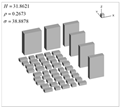
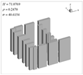
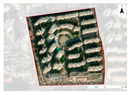
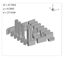
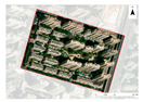
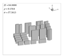
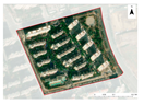
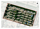
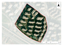
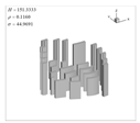
To address this gap, this study conducts a detailed survey of urban morphology in Hefei, China, and selects 20 real building blocks with diverse height, density, and standard deviation characteristics. Using CFD simulations, we investigate the impact of realistic height non-uniformity on ventilation efficiency and pollutant dispersion. Compared with previous works that typically focus on abstracted forms or isolated flow effects, this study highlights the importance of morphological synergy—i.e., the combined role of density control and height variability—in shaping vertical airflow dynamics. The results aim to provide technical support for optimizing vertical ventilation corridors in high-density pedestrian zones.
The structure of this paper is as follows: 
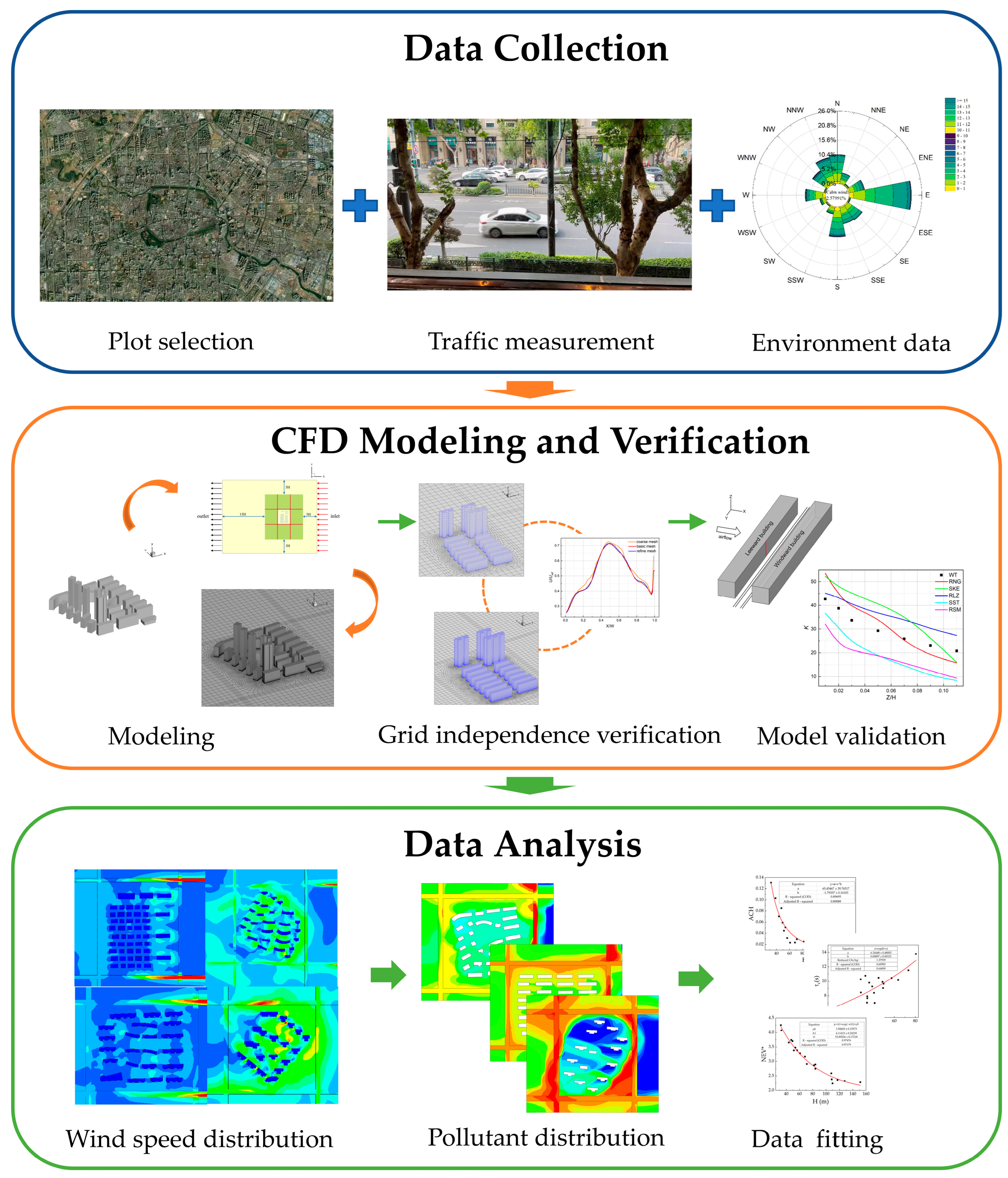
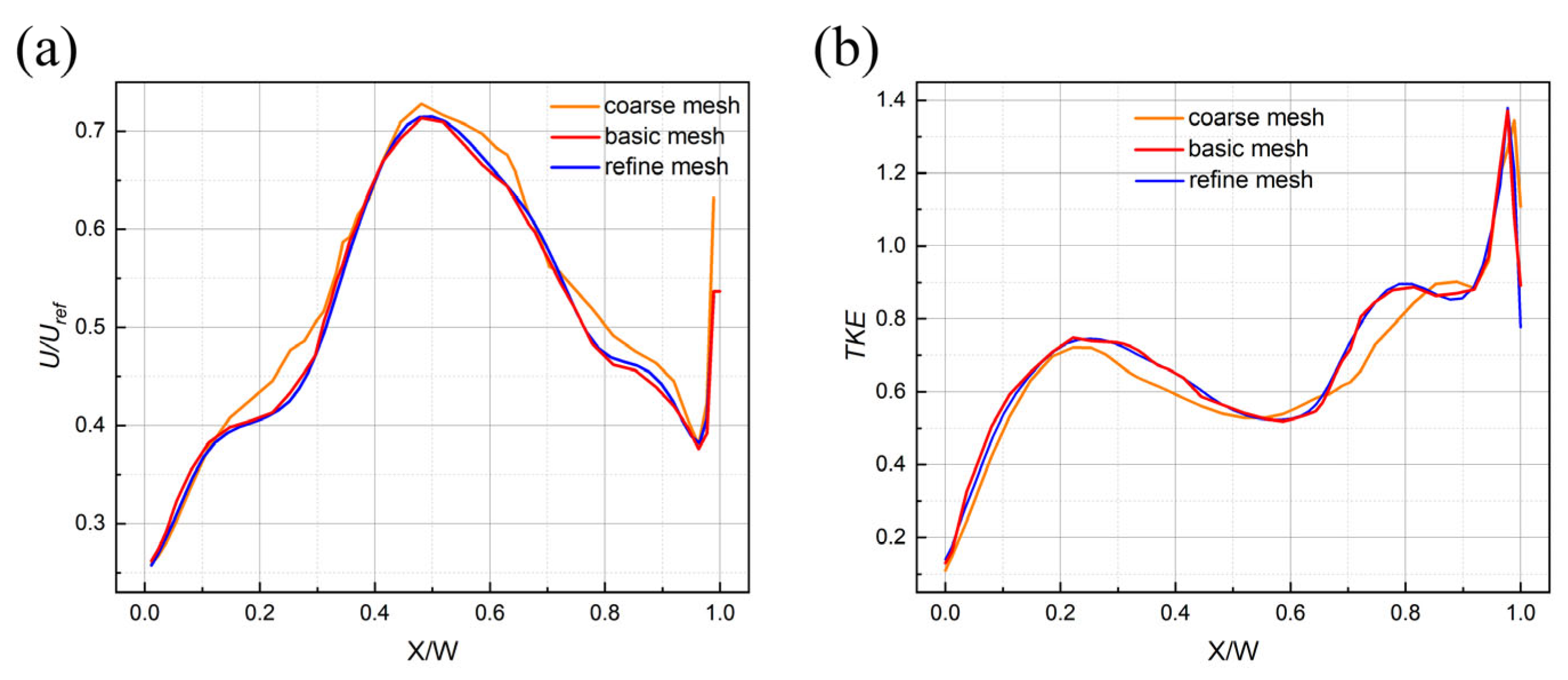
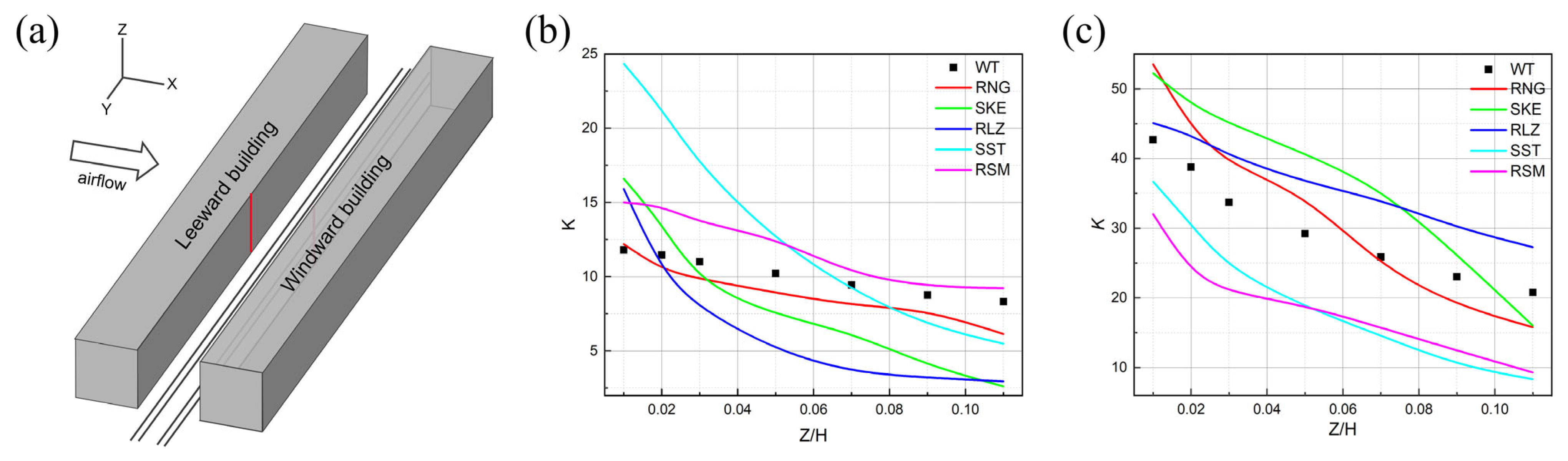
Section 2 presents the details of the physical model, computational domain, boundary conditions, and model validation, including (i) a grid sensitivity study and (ii) a comparison with wind tunnel experiments. In Section 3, ventilation performance and pollutant concentration distributions within the target site and its downstream region are introduced and discussed, based on wind velocity, pollutant transport, air exchange rate (ACH), air residence time (τc), and net escape velocity (NEV*). Section 4 discusses the broader implications of the findings, including the limitations of this study, future research directions, and practical strategies for urban ventilation optimization. Section 5 provides the final conclusions. The specific flow chart is shown in Figure 1.

2. Materials and Methods

2.1. Model Description and Domain Dimensions

In this study, a total of 20 real urban building blocks were selected based on three key influencing factors: average building height (H), building height standard deviation (σ), and building density (ρ). These blocks represent a range of different average heights, densities, and height variability levels, as detailed in Table 1. Due to modeling and simulation constraints, the building densities used in the CFD simulations may differ slightly from the actual densities of the selected blocks. The density values listed in Table 1 refer to the modeled building densities used in the simulations.
Based on COST 732 [20] and AIJ [21] guidelines, and also considering that the actual wind direction in urban areas may vary, the computational domain was set as 5H upstream (H refers to the average height of cases 1–20), 15H downstream, 5H lateral clearance, and 5H in the vertical direction. Taking the computational domain of case 5 as an example, the schematic diagram of the domain is shown in Figure 2, where the yellow area in the middle represents the target block.

2.2. Boundary Condition

The overall urban ventilation and pollutant dispersion are greatly affected by the city’s prevailing wind direction throughout the year. According to the Standard Meteorological Data Handbook for Building Applications [22], statistical analysis was conducted for Hefei City. The analysis of wind direction and speed data (see Figure 3) shows that the prevailing wind throughout the year is from the east. Therefore, in this study, the due east wind direction—corresponding to the negative x-direction in Figure 2—is used for simulations.
In this study, a user-defined function (UDF) was used to implement the inlet velocity profile. The inlet velocity profile was simulated using the power law. The following definitions apply to the inlet velocity, turbulent kinetic energy (k), and turbulence dissipation rate (ε):
U z = U r e f Z Z r e f α
k = U Z I Z 2
ε = C μ 3 / 4 k 3 / 2 κ z
Among them, Uref (m/s) represents the average wind speed corresponding to the height Zref. It is taken as 3 m/s. According to the national building structure load code standard [23], α is taken as 0.22, corresponding to the urban area with dense building groups. The parameter IZ represents the turbulence intensity at height Z, H is the building height, Zref is the reference height (36 m), Cμ = 0.08445, and κ = 0.04 is the von Karman constant.
The building surfaces and the bottom boundary of the domain were defined as no-slip wall boundary conditions. The top and lateral boundaries of the domain were set as symmetry boundaries. The outlet boundary is assumed to be a pressure outlet, and the normal gradients of all variables at the outlet boundary are set to zero. Additionally, considering the impact of pollutants within the streets on the surrounding building clusters, this study also set pollution sources around the building clusters. The pollution sources were modeled with a 4-lane configuration, 18 m width, and emission height set at 1.5 m (pedestrian level). The source strength was calculated based on field investigations (see Appendix A), and the source locations are marked in red in Figure 2. The ground pollution sources were defined as continuous line sources, with lengths equal to the street canyon length and aligned parallel to the canyon’s spanwise direction. Carbon monoxide (CO) was selected as the representative pollutant. The line source emission rates were determined based on field traffic flow data from Hefei (see Appendix A) and emission factors provided in reference [24]. The total traffic pollutant emissions were set as 0.4389 × 10⁻⁶ Kg/(m3·s), and the pollutant concentration at the inlet boundary was set to zero.
To simulate the influence of the surrounding building clusters on the target site, the building clusters around the target site were simplified as a porous medium zone. The height of the porous medium block was set based on H values obtained from urban surveys in Hefei. The length and width of the porous block were made equal to those of the target site. The porous medium region is indicated by the green area in Figure 2.

2.3. Grid Independence Verification

Mesh generation is a crucial step in numerical simulations, as the selection of grid types and the size of grid elements significantly influence simulation results [25]. In this study, the generation of the computational grid was based on the surface-extrusion technology proposed by van Hooff and Blocken [26]. The computational grid exclusively employs structured grids, with the minimum grid size ranging from 1/40 to 1/60 of the H. Grid refinement was applied around the building models, and the grid spacing expanded at a growth rate of 1.1–1.2. The near-wall flow is within the logarithmic law layer, which satisfies the conditions for applying the wall function approach because the dimensionless wall distance y+ from the first-layer grid node near the wall to the wall is primarily in the range of 50–180. Based on reports by Franke et al. [20] and Tominaga et al. [21], the fourth grid layer from the ground was located at a pedestrian height of 1.5 m. To verify grid quality, a sensitivity analysis was carried out. Three grid systems were tested: a coarse grid (2.46 million cells), a medium grid (4.52 million cells), and a fine grid (8.71 million cells). The computational domain grids were entirely divided into hexahedral cells, with a schematic comparison shown in Figure 4. The velocity fields and turbulent kinetic energy variations along the central axis at the top of the domain for the three grid systems are presented in Figure 5. The results demonstrate minimal differences in velocity fields and turbulent kinetic energy between the medium and fine grids, whereas the coarse grid exhibits noticeable deviations compared to the other two systems. Therefore, considering both simulation accuracy and computational efficiency, the medium grid system was selected for subsequent numerical investigations.

2.4. Solution Method

The Semi-Implicit Method for Pressure-Linked Equations (SIMPLE) algorithm is used for the pressure–velocity coupling control equation. The second-order format is used for the pressure interpolation scheme. Second-order discretization schemes are used for both the convection terms and the viscous terms of the governing equations. The double-precision solver is used for CFD calculation. The relaxation factors under the solution equation use the default values. The iteration continues until the relative errors of the conservation equation and the energy equation are both lower than 1 × 10⁻⁵. At this point, the equation is considered to be convergent.

2.5. Model Validation

To validate the rationality of boundary condition settings and select appropriate turbulence models by comparing their simulated wind speed distributions under identical conditions, this study references the atmospheric boundary layer wind tunnel experiments conducted by Gromke and Ruck at the Environmental Aerodynamics Research Center of Karlsruhe Institute of Technology (Karlsruhe, Baden-Württemberg, Germany) on pollutant dispersion in street canyons. Experimental data are available at http://www.codasc.de (accessed on 9 October 2024). Five turbulence models were evaluated: (1) standard k-ε model (SKE); (2) realizable k-ε model (RLZ); (3) RNG k-ε model (RNG); (4) SST k-ω model (SST k-ω); and (5) Reynolds Stress Model (RSM).
The wind tunnel test section was 2 m × 1 m × 2 m (width × height × length). The wind was perpendicular to the street. The street canyon model is composed of two parallel buildings of 0.12 m × 0.12 m × 1.2 m (height × width × length). The scale ratio with the actual street canyon is 1:150. The width of the canyon is 0.12 m. Four pollutant emission line sources are placed on the canyon ground. Sulfur hexafluoride (SF6) is selected as the tracer gas. The concentration on the canyon wall is normalized as follows:
K = C U H H Q S / l
where C is the measured concentration Kg/m3, UH is the flow velocity (m/s) at height H (m), QS is the pollution source intensity (Kg/s), and l is the length of the line source (m).
The size of the simulation setting is equal to that of the wind tunnel. The computational mesh division and solution method follow the method described in Section 2.3. Normalized pollutant concentrations were measured along the center vertical line (red line in Figure 6a) on both leeward and windward sides in the wind tunnel model. These were compared with CFD results using five turbulence models. The comparison results are shown in Figure 6b,c.
To better compare the computational accuracy of the various turbulence models, we selected three validation metrics to quantify the correlation between the wind tunnel experimental data and simulations: fractional bias (FB), root normalized mean square error (RNMSE), and Pearson correlation coefficient (R) [27]. The results are summarized in Table 2. The acceptable range for each indicator can be found in the literature [28].
Figure 6b shows the normalized concentration along the windward side of the street canyon. The three k-ε models predict pollution concentrations that are lower than those found in wind tunnel data. In contrast, the SST and RSM models overestimate the pollutant concentrations on the wall. Figure 6c shows the normalized concentration on the leeward wall of the street canyon. The simulation results are the opposite of those on the windward side. The three k-ε models overestimate pollution concentrations in the wind tunnel experiment. SST and RSM modeling predictions underestimate pollution concentrations in the wind tunnel experiments. Table 2 shows that the RNG model has the lowest absolute values of FB and RNMSE among the five turbulence models, and its correlation coefficient is within an acceptable range. Overall, among the five turbulence models, the RNG model demonstrated the closest agreement with wind tunnel measurements. Therefore, the RNG model was selected for experimental investigations in this study.

3. Results

This section builds upon the model established in Section 2.1. This study analyzes the target site and its impact on downstream building clusters from several aspects. These include wind speed, pollutant dispersion characteristics, and the relationships between urban morphology parameters (H, ρ, and σ) and ventilation metrics such as ACH, τc, and NEV*. Optimization strategies for vertical ventilation corridors are proposed based on numerical simulation results.
The concept of ACH is used in many street canyon ventilation problems. It represents the air exchange volume between the inside and outside of the street canyon per unit time [29]. The ACH of a 3D independent street canyon comprises the following three components [30]:
A C H + = ( A C H T o p + ) + ( A C H S i d e 1 + ) + ( A C H S i d e 2 + )
where ACHTOP+ is the ACH in the positive z-axis direction through the top of the street canyon. ACHSide1+ is the ACH in the positive x-axis direction. ACHSide2+ is the ACH in the negative x-axis direction.
The ventilation performance of the entire street canyon will be evaluated by the canyon τc [31]. The calculation formula is as follows:
Θ = 1 V c d x d y d z
τ c = Θ × V Q
where c is the local concentration of passive tracer gas (kg/m3), Q is the pollutant emission rate (Kg/s), and V is the street canyon volume. The average pollutant concentration Ɵ signifies the overall air quality of the street canyon, whereas τc represents the time scale for a parcel of pollutant being removed from the street canyon.
The ventilation volume in the pedestrian breathing zone is calculated using NEV* as the evaluation factor. The purging flow rate (PFR) (m3/s) calculation formula is as follows [32]:
P F R = Q × V m
where PFR indicates how much fresh air is provided to the area, m is the spatially averaged concentration (kg/m3) of the street canyon, Q is the pollutant release rate (Kg/m3·s), and V is the volume of the considered area.
The calculation formula for NEV* is as follows [33,34]:
N E V p e d = P F R A p e d
N E V * = N E V p e d U r e f
where Aped is the whole area of boundaries of the entire pedestrian respiration volume.

3.1. Wind Speed Distribution

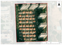
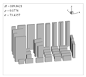
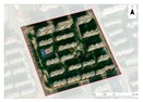
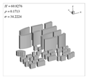
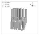
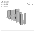
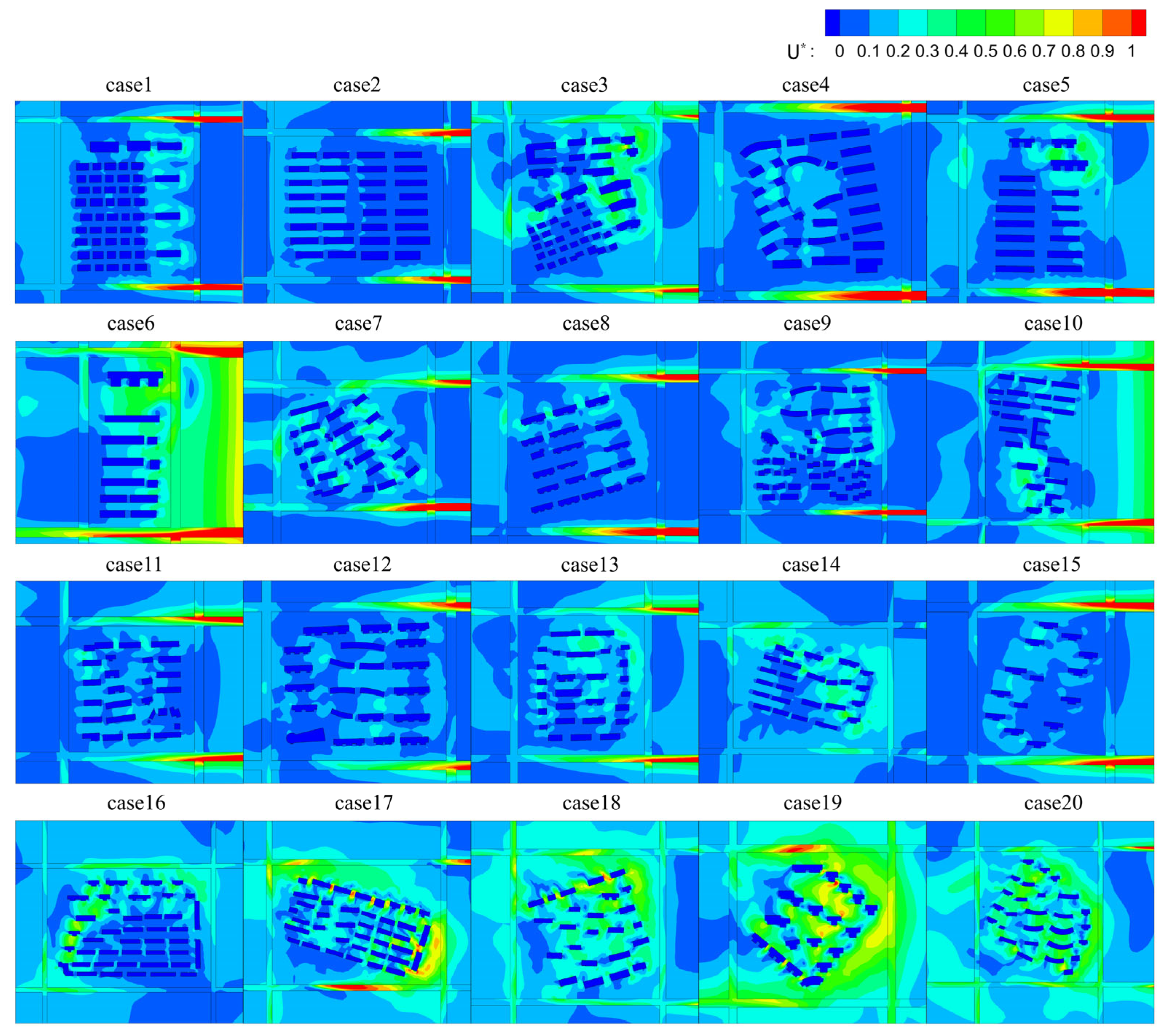
For comparative analysis purposes, the wind speed distribution of height-asymmetric building clusters was analyzed using non-dimensional wind velocity. An analysis was conducted based on the wind speed contour plots at pedestrian height (Z = 1.5 m), as shown in 
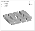
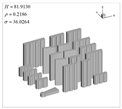
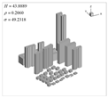
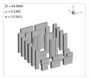
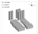
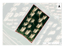
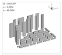
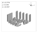
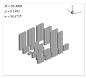
Figure 7. From the wind speed distributions of the 20 selected cases, a clear correlation between wind speed patterns and building height is observed. The overall distribution exhibits a typical gradient characteristic—higher wind speeds at the edges and lower within the interior. This phenomenon results from the blocking and frictional effects of buildings, which gradually dissipate the kinetic energy of the incoming flow, leading to reduced wind speeds as airflow penetrates deeper into the urban block. For example, in case 1, 
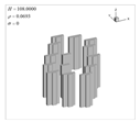
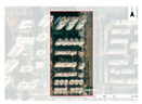
H is relatively low. Both peripheral and interior wind speeds are relatively uniform. High-speed zones are widely distributed along the site edges, allowing smoother wind penetration into the interior. In contrast, case 20 has a much higher H. High-speed zones are limited near the periphery, while elevated wind speeds are observed only within narrow building gaps, indicating that incoming airflow is strongly obstructed, resulting in restricted circulation throughout the block.
Overall, in the low-rise cases (case 1–case 5), the relatively low building heights allow for stable and uniform airflow within the blocks. In the mid-rise cases (case 6–case 15), increasing building heights cause greater fluctuations in wind speed. The obstruction effect becomes more prominent, and the number of low-speed zones within the block increases. Irregular layouts in this group are also more likely to generate stagnant air pockets. In the high-rise cases (case 16–case 20), the wind speed distribution becomes more complex, dominated by strong turbulence and vortex formation. These cases exhibit the most pronounced airflow obstruction. For instance, in case 18 and case 19, the wind speed contour plots reveal high-speed regions above and along the sides of buildings, while significant low-speed and turbulent zones emerge in the wake regions behind them.

3.2. Pollutant Distribution

For the convenience of analysis, a dimensionless concentration is introduced for analysis [32], and the definition of the dimensionless pollutant concentration is as follows:
C * = C U 0 H L Q
where C is the pollutant concentration (Kg/m3), U0 is the flow mean velocity (m/s), H is the building height (m), L is the length of the line source (m), and Q is the total emission (Kg/s).
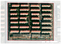
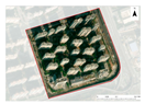
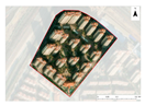
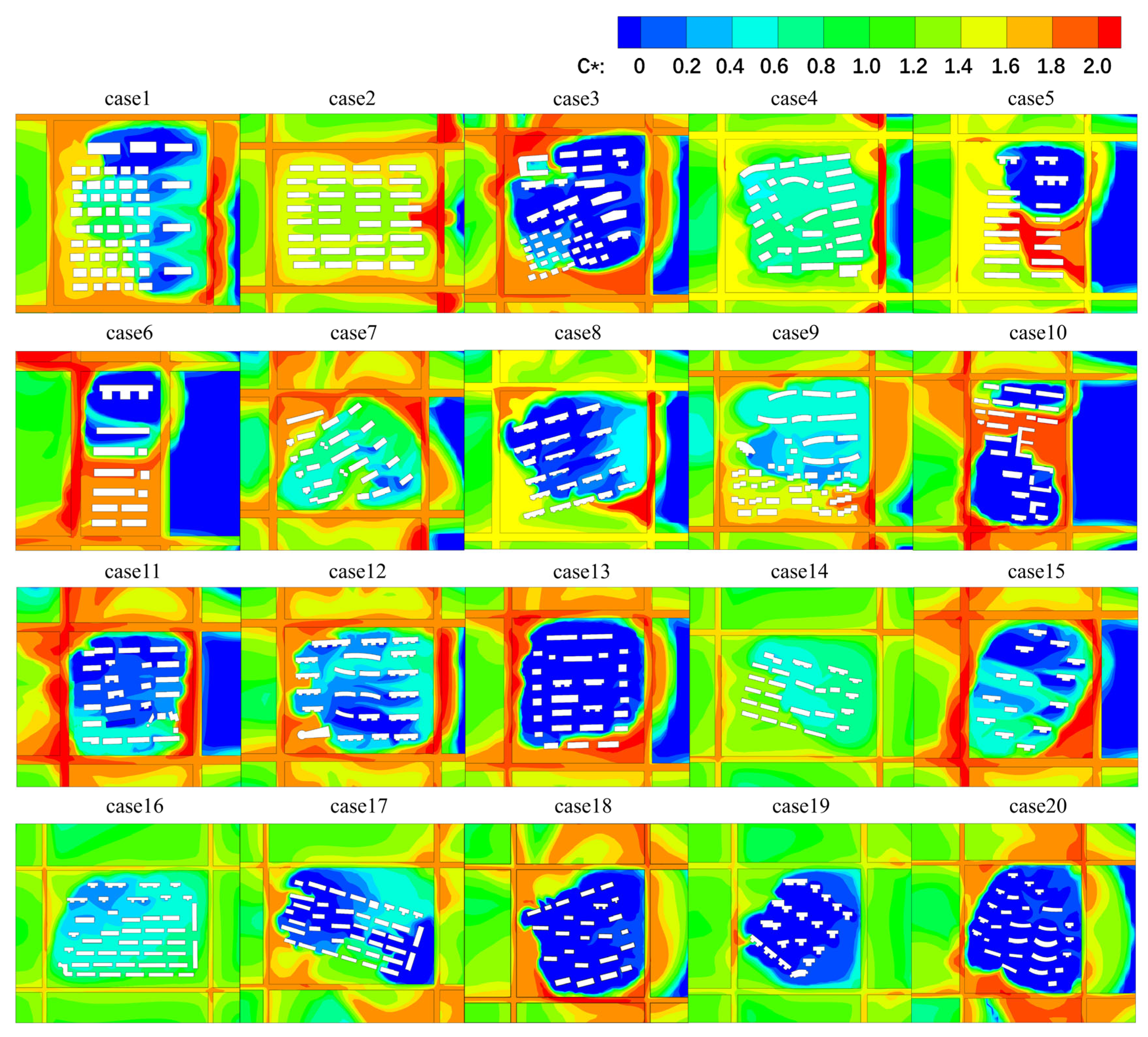
To analyze pollutant distribution patterns at the pedestrian level, this section continues to utilize pollutant concentration contours at Z = 1.5 m (Figure 8). Key findings are as follows: pollutant concentration distributions vary significantly across the 20 sites. This spatial heterogeneity strongly correlates with the layout and morphology of the building clusters. A characteristic edge-elevated, internally heterogeneous distribution pattern dominates the urban fabric.
In low-rise cases (case 1–case 5), smooth airflow and well-formed ventilation pathways contribute to uniformly low pollutant concentrations. For instance, in case 1, buildings are regularly arranged with relatively even spacing, resulting in multiple effective air channels and enhanced pollutant dispersion. Although case 2 also features an orderly layout, elevated concentrations are observed in certain edge areas, likely due to local wind direction or surrounding environmental interference. In mid-rise cases (case 6–case 15), increasing building height leads to more pronounced fluctuations in pollutant concentrations. Airflow obstruction intensifies, especially in dense clusters such as case 9, where pollutant accumulation is evident. Conversely, in more dispersed configurations like case 12, pollutant removal is more efficient due to improved flow continuity. High-rise cases (cases 16–20) show a polarized pattern in pollutant distribution. High concentrations appear around tall building perimeters, while low concentrations are found in interior spaces. This behavior reflects the interplay of several key factors, including the blockage effect of ρ, the capacity for ventilation corridor formation, and proximity to pollutant sources. Edge zones are particularly prone to pollutant buildup due to the combined influence of external inflow and internal recirculation.

3.2.1. Influence of Average Building Height on the Target Block
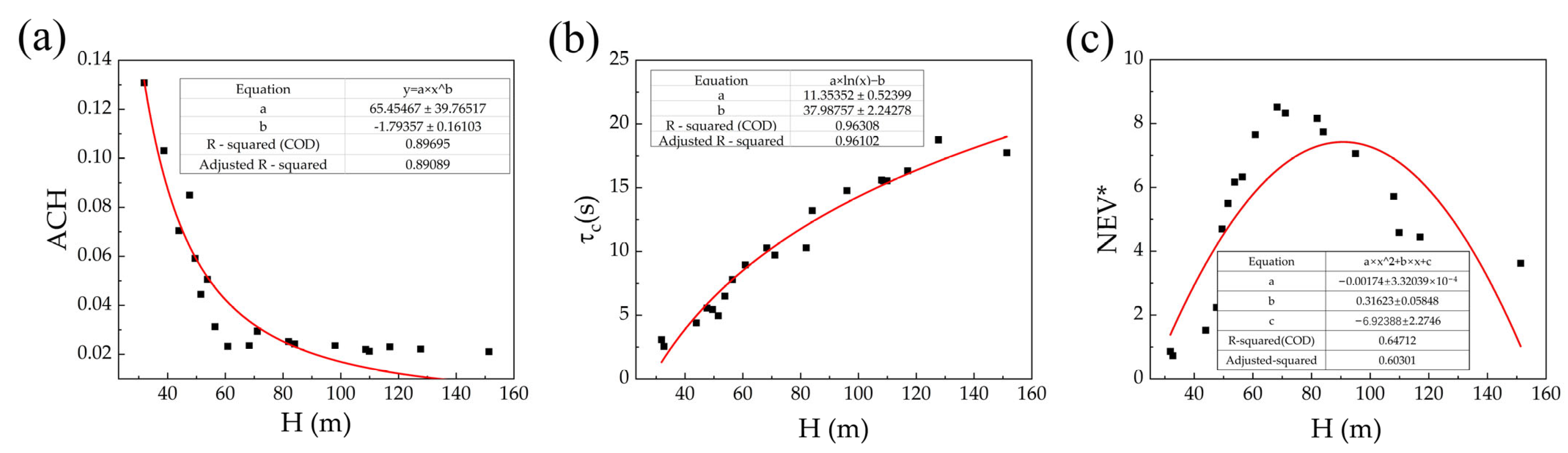
As shown in Figure 9, the relationships between the mean building height of the target site and three ventilation-related parameters—ACH, τc, and NEV*—exhibit clear stage-dependent characteristics. In the low-rise stage (0–60 m), ACH remains relatively high (0.13–0.03 m/s), τc is short (0–10 s), and NEV* gradually increases (1–8). These trends indicate that short buildings offer the least resistance to airflow, enabling horizontal winds to effectively penetrate the site and maintain relatively good ventilation performance. As the H increases to the mid-rise range (60–100 m), all three parameters show marked changes. The ACH drops below 0.025 m/s and tends to stabilize; τc rapidly increases to around 14 s; and NEV* decreases below 7. This suggests the following: Once buildings reach the average urban canopy height, the “street canyon effect” starts to take over. Horizontal ventilation becomes increasingly restricted, while vertical mixing remains insufficient. As a result, there is a significant drop in overall ventilation efficiency.
When building heights exceed 100 m, entering the high-rise stage, the trends diverge. The inlet exchange rate stays low, indicating persistent stagnation near the ground. The growth in τc slows (15–17 s), suggesting a sustained near-ground influence from super-tall buildings. Meanwhile, NEV* shows a modest rebound, increasing from 3 to 5. This reflects the emergence of a “rooftop ventilation effect”. Strong shear flows near the tops of buildings enhance vertical mixing, partially compensating for weak ventilation at ground level. This parameter divergence reveals the formation of a more complex airflow structure in high-rise environments, where near-ground and upper-layer ventilation behave distinctly.
Overall, the results indicate that the 60–100 m height range is a critical threshold for wind environment transition. Below 60 m, the influence of building morphology on airflow is primarily horizontal. Above 100 m, vertical mixing becomes more pronounced. This trend provides important insight into ventilation behavior across different height regimes. Mid-rise clusters are most prone to poor ventilation, while super-tall groups may improve local airflow through enhanced vertical exchange.

3.2.2. Influence of Average Building Height on Downstream Building Group of the Target Block
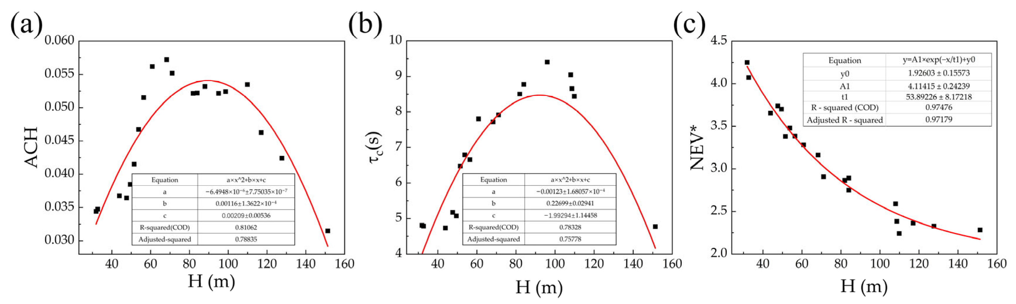
As shown in Figure 10, the relationships between ACH, τc, and NEV* of the downstream building group and the mean building height of the target site are presented. The results reveal that, when analyzed as a single factor, the ventilation performance of the downstream area differs significantly from that of the target site and is more sensitive to changes in upstream building height. The realistic building model does not fully capture the decay of turbulence intensity with distance, which adds complexity to airflow behavior in downstream zones.
For ACH, the downstream group exhibits a much narrower range (0–0.06 m/s) compared to the target site (0–0.15 m/s), with the maximum value reduced by approximately 60%. As the mean height of the target site increases, the downstream ACH rapidly declines. This suggests that although the target site may retain acceptable ventilation, its shielding and disturbance effects substantially weaken the interaction between the downstream group and the ambient wind field. τc in the downstream area also shows a distinct pattern. From Figure 10b, it is evident that under the same average building height, the τc in the downstream building group is generally 25–30% higher than that in the target block. For example, at a height of 40 m, τc in the downstream group exceeds that of the target site by approximately 20%; near 100 m, the downstream area continues to exhibit longer τc. This difference can be attributed mainly to the fact that the downstream group lies within the leeward zone of the target block, where airflow momentum has been substantially dissipated by the upstream buildings, resulting in reduced wind speed. In addition, the shielding effect of the target block promotes the development of recirculation zones downstream, further inhibiting air exchange efficiency. Compared with the target block, the downstream group experiences insufficient rooftop shear flow and vertical ventilation development, making it more prone to pollutant and stagnant air accumulation in the leeward area. Regarding NEV*, the downstream region reaches its maximum (~4.2) when the mean height of the target site is around 40 m, while the peak value at the target site is significantly higher (~8.7). This means the pollutant removal capacity in the downstream area is only about 48% of that in the target site. As the upstream height increases, NEV* in the downstream group declines further, suggesting that pollutants become increasingly difficult to disperse in these zones, thereby obstructing effective urban ventilation pathways.

3.3. Influence of Building Density on the Target Block and Its Downstream Building Group

As shown in Figure 11, the relationships between ρ of the target site and three key ventilation indicators—τc, NEV*, and τc in the downstream building group—are analyzed. The results indicate that τc in the target site exhibits a significant exponential correlation with ρ (R2 = 0.9157). As the density increases from 0.10 to 0.30, τc rises sharply from 5.5 s to over 16 s, an increase of more than 190%. This confirms that high-density building configurations severely obstruct airflow, intensifying pollutant retention and reducing ventilation efficiency. In the low-density range (ρ < 0.15), the target site’s τc is 20–35% lower than that of the downstream area, indicating better airflow and weaker blockage effects. Furthermore, the density–τc relationship in the downstream group appears linear, while that of the target site follows a distinct exponential trend. This contrast suggests a lagged ventilation response in the downstream region, where wind field regulation is less sensitive compared to the target site.
In contrast, the relationship between NEV* and ρ shows obvious segmented changes. In the low-density stage (ρ < 0.13), NEV* gradually increases and reaches a peak (around 11) within a specific density range. Beyond this critical point (ρ > 0.15), NEV* drops sharply and stabilizes between 1 and 2; the lowest value falls below 1.0, which is only about 9% of the peak. This trend implies that within a certain density range, structural airflow channels may be triggered, enhancing pollutant dispersion. However, once the density exceeds this threshold, such ventilation pathways collapse, leading to a drastic drop in escape efficiency.
Cross-analysis between ρ and H further reveals that when H > 90 m and ρ > 0.20, the downstream group’s τc exceeds that of the target site by approximately 25–40%. This indicates that the combined effect of height and density significantly impedes local air renewal. Two primary reasons may explain this: (i) taller buildings intensify shielding and recirculation effects on the leeward side; (ii) high-density layouts hinder ventilation corridor formation and reduce both horizontal and vertical wind continuity. As the downstream group is situated on the leeward side of the prevailing wind, pollutant accumulation and air stagnation are more likely. By contrast, the target site, being more exposed to wind pressure and lateral flow, experiences slower increases in τc. Under the combined condition of H ≈ 90 m and ρ ≈ 0.2, the downstream area’s τc is 32% higher than that of the target site, further confirming the amplified shielding effect and wind stagnation accumulation in leeward zones.

3.4. Influence of Building Height Standard Deviation on the Target Block and Its Downstream Building Group

3.4.1. Influence of Building Height Standard Deviation on the Target Block

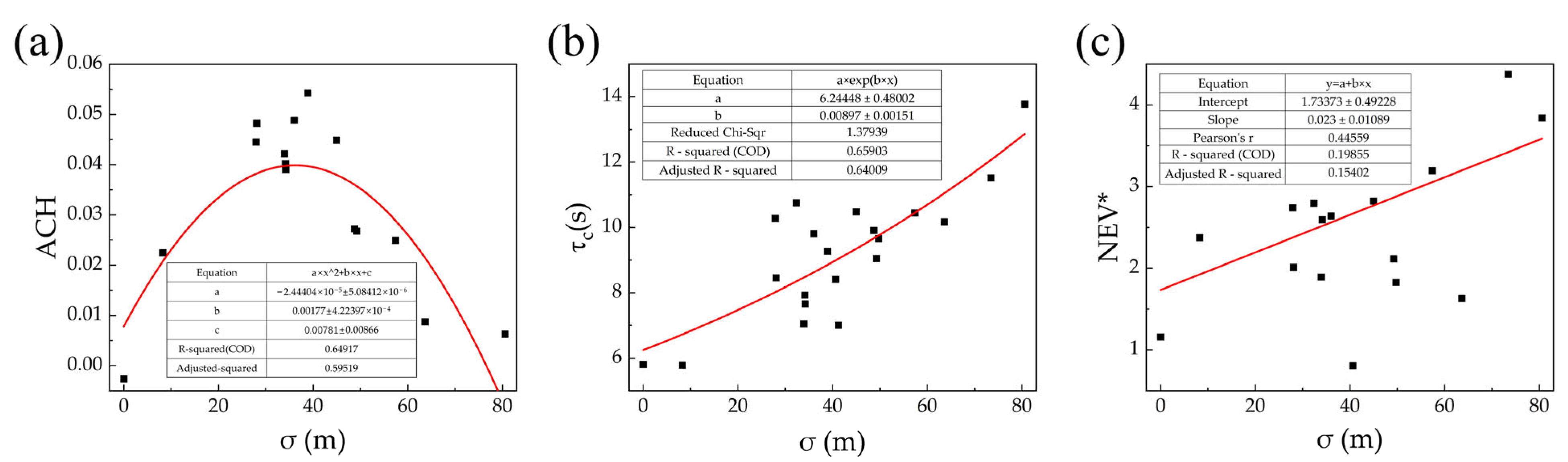
Figure 12 illustrates the relationships between σ and three key ventilation parameters at the target site: ACH, τc, and NEV*.
As shown in Figure 12a, ACH exhibits a distinct parabolic relationship with σ (R2 = 0.69). This indicates that height variability significantly influences wind-driven ventilation at the site entrance. As the σ increases, the ACH first rises and then declines, reaching its peak around σ ≈ 30–40 (m). This suggests the presence of an “optimal range” of height variation for enhancing airflow penetration and promoting vertical disturbance at the site boundary. Figure 12b shows that τc increases exponentially with σ (m). When σ > 50 (m), τc rises sharply, suggesting that larger height differences cause stronger disturbances in the upper wind profile. In such cases, some taller buildings may induce a “cap effect”, impeding the smooth dispersion of air in upper layers. Thus, excessive height variability is detrimental to upper-level ventilation. Figure 12c demonstrates an exponential decay between NEV* and σ. As σ (m) increases, NEV* rapidly declines, a trend consistent with the increase in τc observed in Figure 12b. This further confirms that although significant height variation can enhance local turbulence at the lower level, it restricts the overall pollutant removal path, making it more difficult for air to escape into the atmospheric boundary layer.
The coupling between ρ and height variability reveals a clear threshold effect in ventilation regulation. When ρ < 0.15, σ = 30~50 (m) can effectively enhance ACH (Figure 11a), elevate NEV* to a local peak (Figure 11b), and significantly reduce τc (Figure 11a). These results indicate that under low-density conditions, height variability can effectively induce turbulent disturbances, thereby improving ventilation performance within the building cluster. However, as ρ continues to increase—especially beyond 0.20—even when σ remains in its optimal range, ACH declines sharply (Figure 12a), τc continues to rise (Figure 12b), and NEV* drops significantly (Figure 12c). This demonstrates that ρ is the key factor limiting the ventilation regulation effect of σ. In high-density environments, the ventilation benefits induced by height variations are offset by the overall enclosure characteristics of the building cluster morphology. In conclusion, urban form optimization should consider the coupled mechanism of “vertical perturbation–lateral resistance”. Coordinated control of ρ and height heterogeneity can jointly enhance vertical ventilation performance.

3.4.2. Influence of Building Height Standard Deviation on the Downstream Building Group of the Target Block

Figure 13 illustrates the relationships between σ of the downstream building group and three ventilation parameters: ACH, τc, and NEV*. The plots reveal functional dependencies between σ (m) and these parameters in the downstream building group, though with weaker statistical significance and regularity compared to the target site. Specifically, ACH follows a parabolic trend with σ (m) (Figure 12a), peaking at σ ≈ 35–40 (m) (≈0.04 m/s). This peak value is 20% lower than that observed in the target site, indicating that while an “optimal σ (m)” exists for vertical perturbation in the downstream building group, its effectiveness is significantly constrained by the upstream target site. This optimal range of σ ≈ 35–40 likely reflects a balance between promoting vertical turbulence and maintaining pathway continuity for airflow. Moderate height variability breaks up horizontal stagnation zones and enhances upward mixing, while avoiding the excessive obstruction caused by highly irregular building forms. τc exhibits an exponential increase with σ, accelerating when σ > 50 (m). This suggests excessive height variations create pronounced reverse pressure zones and recirculation bands between buildings, obstructing upper-level air escape pathways and prolonging ventilation cycles. NEV* shows a weakly correlated positive trend with σ (m) (R2 = 0.15402), implying substantial interference from external factors. Nevertheless, the general trend confirms that moderate height variations enhance vertical gas escape, though this effect saturates or even diminishes beyond a critical σ (m) threshold. In conclusion, σ (m) holds potential for regulating local vertical ventilation, but its efficacy is closely tied to ρ. In high-density clusters, increasing height variations alone fail to mitigate overall ventilation deficits and may instead amplify recirculation due to intensified local perturbations.

4. Discussion

Although this study systematically analyzes the effects of average building height, density, and height variability on ventilation and pollutant dispersion based on realistic urban blocks, several limitations remain. First, the limited number of samples may not fully represent the diversity of urban forms. Second, the simulations did not account for wind direction variability, internal heat sources, or the influence of vegetation, all of which may interact with airflow. Moreover, the potential interdependence between building density and height variation warrants further decoupled analysis. Future research should expand the study scope to include multiple cities and climate conditions, incorporate multi-directional wind scenarios across the year, and integrate factors such as energy consumption and pollutant source intensity to build a more comprehensive urban microclimate framework. Practically, urban design should limit excessive building density while introducing moderate height variation (with a recommended standard deviation of 35–40), maintain uninterrupted ventilation corridors along prevailing winds, and avoid overly enclosed configurations. In poorly ventilated areas, staggered and well-spaced building arrangements are recommended to improve airflow exchange and enhance urban wind environments in high-density zones.

5. Conclusions

This study investigates 20 real urban building blocks using a porous media modeling approach, based on variations in H, ρ, and σ. The focus is placed on analyzing ventilation and pollutant dispersion within both height-nonuniform building groups and their downstream (leeward) areas. The main findings are as follows:
(1)
In low-rise areas, wind speed is relatively high, and pollutant concentration is low and evenly distributed. In mid-rise areas, wind speed fluctuates significantly, and pollutant accumulation is more evident. In high-rise areas, wind fields become increasingly complex, with prominent turbulence effects. As building height increases, wind speed distribution becomes more sensitive to various factors, and turbulence intensifies, especially in tall-building clusters;
(2)
The study finds that a height standard deviation between 35 and 40 corresponds to the optimal ventilation performance in the target site. Both lower and higher values outside this range tend to hinder airflow penetration and pollutant dispersion;
(3)
Urban form optimization should be based on a coordinated mechanism between vertical disturbance and horizontal resistance, in which building density and height variability are jointly regulated to enhance vertical ventilation effectiveness;
(4)
The ventilation and pollutant dispersion performance of downstream building groups is heavily influenced by the morphological characteristics of the target (upwind) site.

Author Contributions

Conceptualization, methodology, T.S.; software, writing—original draft preparation, L.C.; formal analysis, writing—review and editing, L.C. and T.X.; supervision, S.Z. All authors have read and agreed to the published version of the manuscript.

Funding

The research was supported by the National Nature Science Foundation of China (No. 52008001), the Housing and Urban–Rural Construction Science and Technology Planned Projects of Anhui Province (No. 2022-YF045), and the Open Project Program of BIM Engineering Centre of Anhui Province (Grant No. AHBIM2022ZR01).

Institutional Review Board Statement

Not applicable.

Informed Consent Statement

Not applicable.

Data Availability Statement

Data available on request.

Acknowledgments

We are thankful to all our colleagues and co-authors for their very valued contributions to this work. The authors are also very appreciative of the reviewers’ comments, which helped better the manuscript.

Conflicts of Interest

The authors declare no conflicts of interest.

Abbreviations

ACHAir exchange rate
τ c Air residence time
NEV*Net escape velocity
HAverage building height
σBuilding height standard deviation
ρBuilding density
SKEStandard k-ε model
RLZRealizable k-ε model
RNGRNG k-ε model
SST k-ωSST k-ω model
RSMReynolds Stress Model
FBFractional bias
RNMSERoot normalized mean square error
RPearson correlation coefficient

Appendix A

In this study, the Changjiang Middle Road (main road) in Hefei City was selected as the research object based on an actual investigation and street comparison according to the street canyon and requirements for pollutant emissions from 0:00 to 24:00 on 11 August 2023 in Beijing Time (UTC+8). Pollutant emissions at the selected measurement points were monitored; that is, traffic flow data were measured on the spot (see Figure A1). The number of cars does not include new energy vehicles. According to the emission factors of different vehicle models based on the literature [28], the total emission of the selected street was calculated to be 0.4389 × 10⁻⁶ Kg/(m3·s).
Figure A1. Average vehicle flow diagram at the measurement points of the main road.
Atmosphere 16 00614 g0a1

References

  1. Sin, C.H.; Luo, Y.; Jon, K.S.; Cui, P.Y.; Huang, Y.D. Effects of void deck on the airflow and pollutant dispersion in 3D street canyons. Environ. Sci. Pollut. Res. Int. 2022, 29, 89358–89386. [Google Scholar] [CrossRef] [PubMed]
  2. Chen, L.; Mak, C.M. Numerical evaluation of pedestrian-level wind comfort around “lift-up” buildings with various unconventional configurations. Build. Environ. 2021, 188, 107429. [Google Scholar] [CrossRef]
  3. Ming, T.; Shi, T.; Han, H.; Liu, S.; Wu, Y.; Li, W.; Peng, C. Assessment of pollutant dispersion in urban street canyons based on field synergy theory. Atmos. Pollut. Res. 2021, 12, 341–356. [Google Scholar] [CrossRef]
  4. López-Pérez, E.; Hermosilla, T.; Carot-Sierra, J.-M.; Palau-Salvador, G. Spatial determination of traffic CO emissions within street canyons using inverse modelling. Atmos. Pollut. Res. 2019, 10, 1140–1147. [Google Scholar] [CrossRef]
  5. Xu, H.; Yan, C.; Fu, Q.; Xiao, K.; Yu, Y.; Han, D.; Wang, W.; Cheng, J. Possible environmental effects on the spread of COVID-19 in China. Sci. Total Environ. 2020, 731, 139211. [Google Scholar] [CrossRef]
  6. Ahmadi, M.; Sharifi, A.; Dorosti, S.; Jafarzadeh Ghoushchi, S.; Ghanbari, N. Investigation of effective climatology parameters on COVID-19 outbreak in Iran. Sci. Total Environ. 2020, 729, 138705. [Google Scholar] [CrossRef]
  7. Hang, J.; Li, Y. Ventilation strategy and air change rates in idealized high rise compact urban areas. Build. Environ. 2010, 45, 2754–2767. [Google Scholar] [CrossRef]
  8. Tominaga, Y. Visualization of city breathability based on CFD technique: Case study for urban blocks in Niigata City. J. Vis. 2012, 15, 269–276. [Google Scholar] [CrossRef]
  9. Wang, W.; Ng, E.; Yuan, C.; Raasch, S. Large-eddy simulations of ventilation for thermal comfort—A parametric study of generic urban configurations with perpendicular approaching winds. Urban Clim. 2017, 20, 202–227. [Google Scholar] [CrossRef]
  10. Ishida, Y.; Okaze, T.; Mochida, A. Influence of urban configuration on the structure of kinetic energy transport and the energy dissipation rate. J. Wind Eng. Ind. Aerodyn. 2018, 183, 198–213. [Google Scholar] [CrossRef]
  11. Hang, J.; Li, Y.; Sandberg, M.; Buccolieri, R.; DI Sabatino, S. The influence of building height variability on pollutant dispersion and pedestrian ventilation in idealized high-rise urban areas. Build. Environ. 2012, 56, 346–360. [Google Scholar] [CrossRef]
  12. Goulart, E.; Reis, N.; Lavor, V.; Castro, I.; Santos, J.; Xie, Z. Local and non-local effects of building arrangements on pollutant fluxes within the urban canopy. Build. Environ. 2019, 147, 23–34. [Google Scholar] [CrossRef]
  13. Zeng, F.; Simeja, D.; Ren, X.; Chen, Z.; Zhao, H. Influence of Urban Road Green Belts on Pedestrian-Level Wind in Height-Asymmetric Street Canyons. Atmosphere 2022, 13, 1285. [Google Scholar] [CrossRef]
  14. Oke, T.R. Street design and urban canopy layer climate. Energy Build. 1988, 11, 103–113. [Google Scholar] [CrossRef]
  15. Meena, R.K.; Raj, R.; Anbukumar, S.; Khan, M.I.; Khatib, J.M. Fluid Dynamic Assessment of Tall Buildings with a Variety of Complicated Geometries. Buildings 2024, 14, 4081. [Google Scholar] [CrossRef]
  16. Yoshida, T.; Takemi, T.; Horiguchi, M. Large-eddy-simulation study of the effects of building-height variability on turbulent flows over an actual urban area. Bound.-Layer Meteorol. 2018, 168, 127–153. [Google Scholar] [CrossRef]
  17. Antoniou, N.; Montazeri, H.; Wigo, H.; Neophytou, M.K.-A.; Blocken, B.; Sandberg, M. CFD and wind-tunnel analysis of outdoor ventilation in a real compact heterogeneous urban area: Evaluation using “air delay”. Build. Environ. 2017, 126, 355–372. [Google Scholar] [CrossRef]
  18. Takemi, T.; Yoshida, T.; Horiguchi, M.; Vanderbauwhede, W. Large-Eddy-simulation analysis of airflows and strong wind hazards in urban areas. Urban Clim. 2020, 32, 100625. [Google Scholar] [CrossRef]
  19. Fang, H.; Ji, X.; Wang, J.; Lu, J.; Yang, M.; Li, J.; Duan, Z. Numerical Simulation and Optimization of Outdoor Wind Environment in High-Rise Buildings Zone of Xuzhou City. Buildings 2025, 15, 264. [Google Scholar] [CrossRef]
  20. Franke, J.; Hellsten, A.; Schlunzen, K.H.; Carissimo, B. The COST 732 Best Practice Guideline for CFD simulation of flows in the urban environment: A summary. Int. J. Environ. Pollut. 2011, 44, 419–427. [Google Scholar] [CrossRef]
  21. Tominaga, Y.; Mochida, A.; Yoshie, R.; Kataoka, H.; Nozu, T.; Yoshikawa, M.; Shirasawa, T. AIJ guidelines for practical applications of CFD to pedestrian wind environment around buildings. J. Wind Eng. Ind. Aerod 2008, 96, 1749–1761. [Google Scholar] [CrossRef]
  22. Zhang, Q.Y.; Yang, H.X. Standard Meteorological Data Handbook for Building Applications; China Architecture & Building Press: Beijing, China, 2012. [Google Scholar]
  23. GB 50009-2012; Load Code for the Design of Building Structures. China Architecture and Building Press: Beijing, China, 2012.
  24. Wang, T.; Xie, S. Assessment of traffic-related air pollution in the urban streets before and during the 2008 Beijing Olympic games traffic control period. Atmos. Environ. 2009, 43, 5682–5690. [Google Scholar] [CrossRef]
  25. Xie, X.; Huang, Z. Impact of aspect ratio and surface heating on pollutant transport in street canyons. J. Mech. Sci. Technol. 2007, 21, 1781–1790. [Google Scholar] [CrossRef]
  26. Van Hooff, T.; Blocken, B. Coupled urban wind flow and indoor natural ventilation modelling on a high-resolution grid: A case study for the Amsterdam Aren A stadium. Environ. Model. Softw. 2010, 25, 51–65. [Google Scholar] [CrossRef]
  27. Miao, Y.; Liu, S.; Zheng, Y.; Wang, S.; Li, Y. Numerical Study of Traffic Pollutant Dispersion within Different Street Canyon Configurations. Adv. Meteorol. 2014, 2014, 1–14. [Google Scholar] [CrossRef]
  28. Moonen, P.; Gromke, C.; Dorer, V. Performance assessment of large eddy simulation (LES) for modeling dispersion in an urban street canyon with tree planting. Atmos. Environ. 2013, 75, 66–76. [Google Scholar] [CrossRef]
  29. Li, X.X.; Liu, C.H.; Leung, D.Y.C. Development of a model for the determination of air exchange rates for street canyons. Atmos. Environ. 2005, 39, 7285–7296. [Google Scholar] [CrossRef]
  30. Mei, S.-J.; Luo, Z.; Zhao, F.-Y.; Wang, H.-Q. Street canyon ventilation and pollution dispersion: 2-D versus 3-D CFD simulations. Sustain. Cities Soc. 2019, 50, 101700. [Google Scholar] [CrossRef]
  31. Cheng, W.C.; Liu, C.H.; Leung, D.Y.C. Computational formulation for the evaluation of street canyon ventilation and pollutant removal performance. Atmos. Environ. 2008, 42, 9041–9051. [Google Scholar] [CrossRef]
  32. Bady, M.; Kato, S.; Huang, H. Towards the application of indoor ventilation efficiency indices to evaluate the air quality of urban areas. Build. Environ. 2008, 43, 1991–2004. [Google Scholar] [CrossRef]
  33. Lim, E.; Ito, K.; Sandberg, M. New ventilation index for evaluating imperfect mixing conditions—Analysis of net escape velocity based on rans approach. Build. Environ. 2013, 61, 45–56. [Google Scholar] [CrossRef]
  34. Hang, J.; Wang, Q.; Chen, X.; Sandberg, M.; Zhu, W.; Buccolieri, R.; Di Sabatino, S. City breathability in medium density urban-like geometries evaluated through the pollutant transport rate and the net escape velocity. Build. Environ. 2015, 94, 166–182. [Google Scholar] [CrossRef]
Figure 1. Flow chart.
Atmosphere 16 00614 g001
Figure 2. Case 5 model computational domain.
Atmosphere 16 00614 g002
Figure 3. Annual wind speed and direction statistical wind rose diagram for Hefei City.
Atmosphere 16 00614 g003
Figure 4. (a) Coarse mesh; (b) medium mesh; (c) fine mesh: detailed partial division diagram of case 5.
Atmosphere 16 00614 g004
Figure 5. Comparison of (a) average velocity and (b) turbulent kinetic energy among coarse, medium, and fine meshes in case 5.
Atmosphere 16 00614 g005
Figure 6. (a) Wind tunnel experiment model (The red line represents the measurement position); comparison of normalized concentrations of simulated data between (b) windward wall and (c) leeward wall and wind tunnel experiment data.
Atmosphere 16 00614 g006
Figure 7. The normalized wind velocity U* = U/Uref at 1.5 m pedestrian height.
Atmosphere 16 00614 g007
Figure 8. The dimensionless concentration (C*) fields at 1.5 m pedestrian height.3.3. Influence of Average Building Height on the Target Block and Its Downstream Building Group.
Atmosphere 16 00614 g008
Figure 9. Relationship between average building height of the target block and (a) air exchange rate; (b) air residence time; (c) net escape velocity.
Atmosphere 16 00614 g009
Figure 10. Relationship between the downstream building group and the target block’s average building height in terms of (a) air exchange rate; (b) air residence time; (c) net escape velocity.
Atmosphere 16 00614 g010
Figure 11. Relationship between the building density of the target block and (a) air residence time of the target block; (b) net escape velocity of the target block; (c) air residence time of the downstream building group.
Atmosphere 16 00614 g011
Figure 12. Relationship between height standard deviation of the target block and (a) air exchange rate; (b) air residence time; (c) net escape velocity.
Atmosphere 16 00614 g012
Figure 13. Relationship between the downstream building group and the target block’s height standard deviation in terms of (a) air exchange rate; (b) air residence time; (c) net escape velocity.
Atmosphere 16 00614 g013
Table 1. Detailed information of the target site.
ConditionsActual ResidencePhysical ModelConditionsActual ResidencePhysical Model
Case 1Atmosphere 16 00614 i001Atmosphere 16 00614 i002Case 11Atmosphere 16 00614 i003Atmosphere 16 00614 i004
Case 2Atmosphere 16 00614 i005Atmosphere 16 00614 i006Case 12Atmosphere 16 00614 i007Atmosphere 16 00614 i008
Case 3Atmosphere 16 00614 i009Atmosphere 16 00614 i010Case 13Atmosphere 16 00614 i011Atmosphere 16 00614 i012
Case 4Atmosphere 16 00614 i013Atmosphere 16 00614 i014Case 14Atmosphere 16 00614 i015Atmosphere 16 00614 i016
Case 5Atmosphere 16 00614 i017Atmosphere 16 00614 i018Case 15Atmosphere 16 00614 i019Atmosphere 16 00614 i020
Case 6Atmosphere 16 00614 i021Atmosphere 16 00614 i022Case 16Atmosphere 16 00614 i023Atmosphere 16 00614 i024
Case 7Atmosphere 16 00614 i025Atmosphere 16 00614 i026Case 17Atmosphere 16 00614 i027Atmosphere 16 00614 i028
Case 8Atmosphere 16 00614 i029Atmosphere 16 00614 i030Case 18Atmosphere 16 00614 i031Atmosphere 16 00614 i032
Case 9Atmosphere 16 00614 i033Atmosphere 16 00614 i034Case 19Atmosphere 16 00614 i035Atmosphere 16 00614 i036
Case 10Atmosphere 16 00614 i037Atmosphere 16 00614 i038Case 20Atmosphere 16 00614 i039Atmosphere 16 00614 i040
Table 2. A quantitative overview of the wind tunnel test.
AimRangeRNGSKERLZSST k-ωRSM
Leeward
wall
FB0|−0.3, 0.3|−0.0767−0.2084−0.18260.39510.4678
RNMSE0 < 1.5 0.07680.20960.18340.40310.6394
R1 < 0.8 0.98830.93400.98430.99910.9751
Windward
wall
FB0|−0.3, 0.3|0.11220.16750.3693−0.3082−0.1768
RNMSE0 < 1.5 0.11230.16810.37570.31190.1774
R1 < 0.8 0.96470.96090.89430.98390.9878
Disclaimer/Publisher’s Note: The statements, opinions and data contained in all publications are solely those of the individual author(s) and contributor(s) and not of MDPI and/or the editor(s). MDPI and/or the editor(s) disclaim responsibility for any injury to people or property resulting from any ideas, methods, instructions or products referred to in the content.

