
Exploring the Influencing Factors of Surface Ozone Variability by Explainable Machine Learning: A Case Study in the Basilicata Region (Southern Italy)


Abstract
1. Introduction
2. Data and Methods
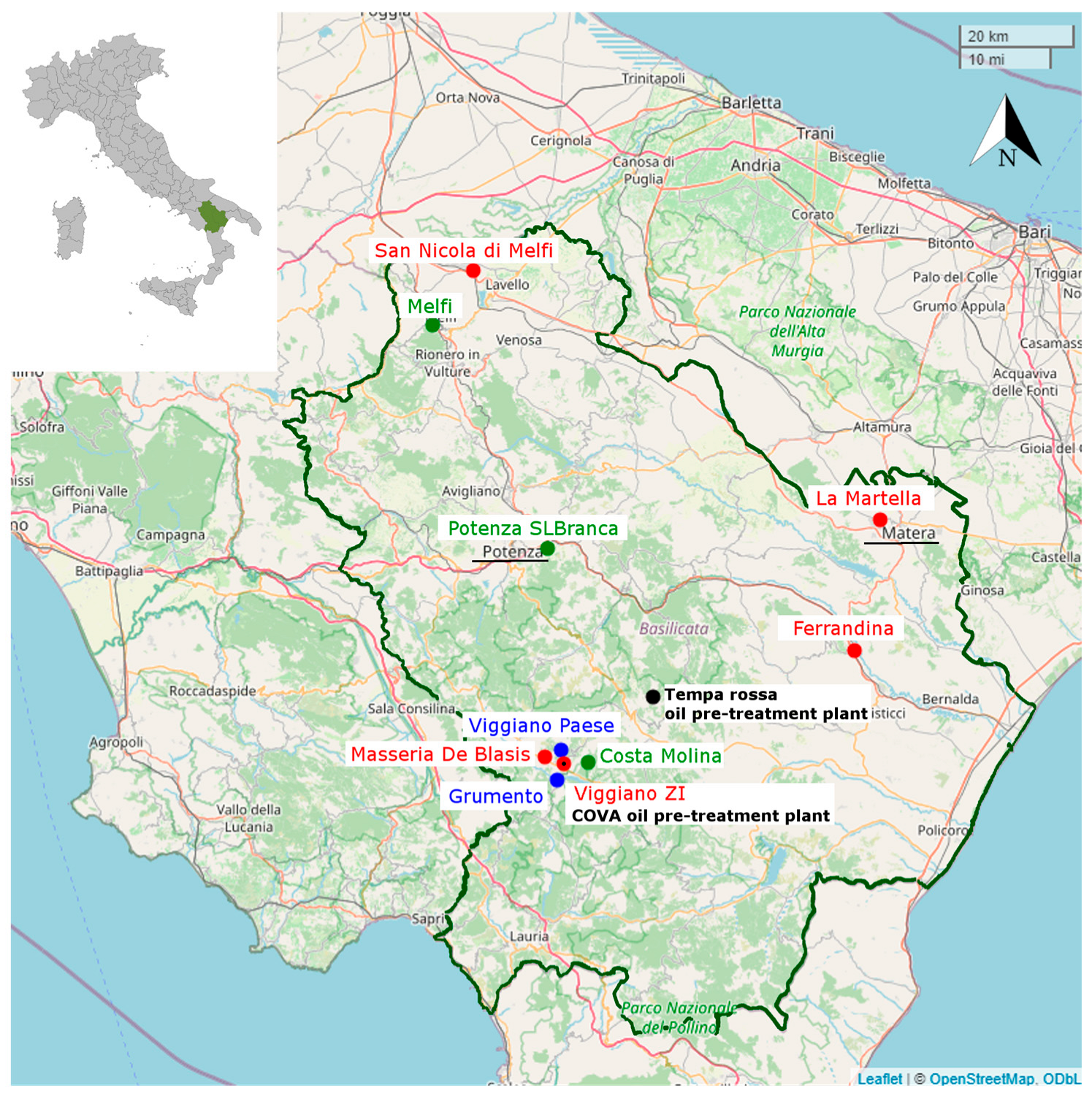
2.1. Study Area
2.2. Observational Dataset
2.3. Machine Learning Models
2.3.1. XGBoost
2.3.2. SHAP
2.3.3. K-Means
3. Results and Discussion
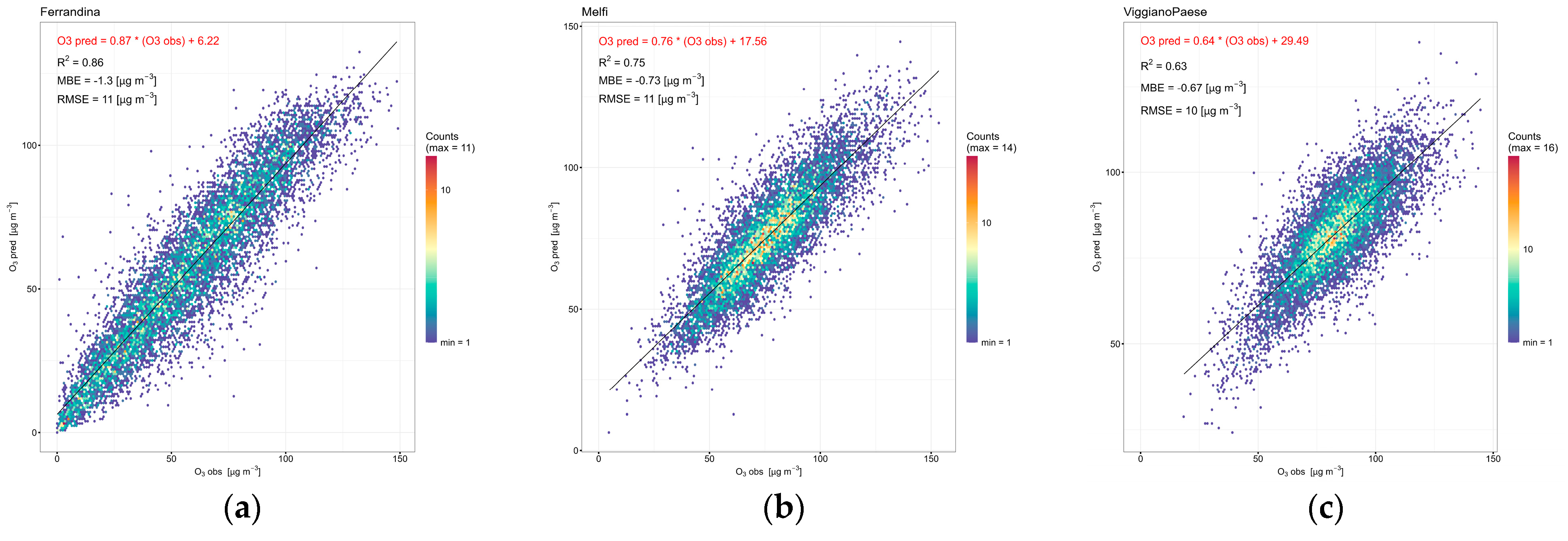
3.1. XGBoost Model Performance
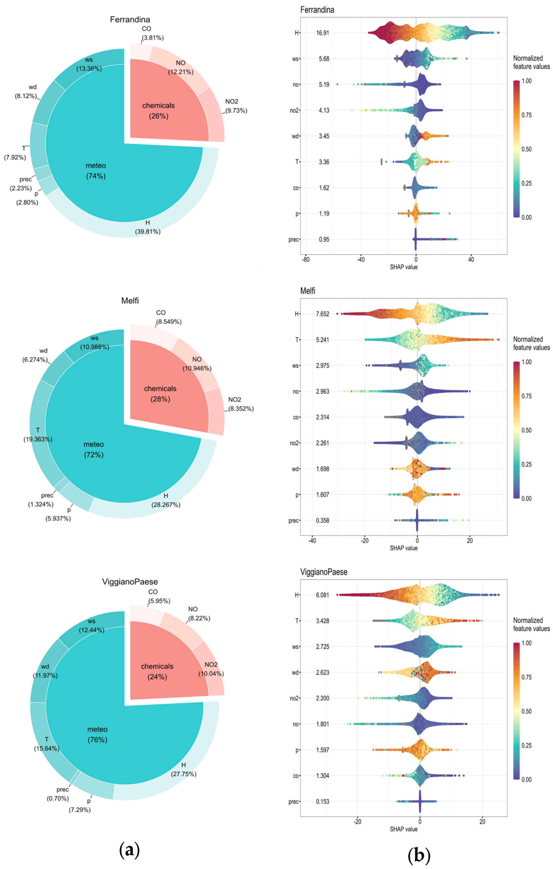
3.2. Global Importance of Main Influencing Factors
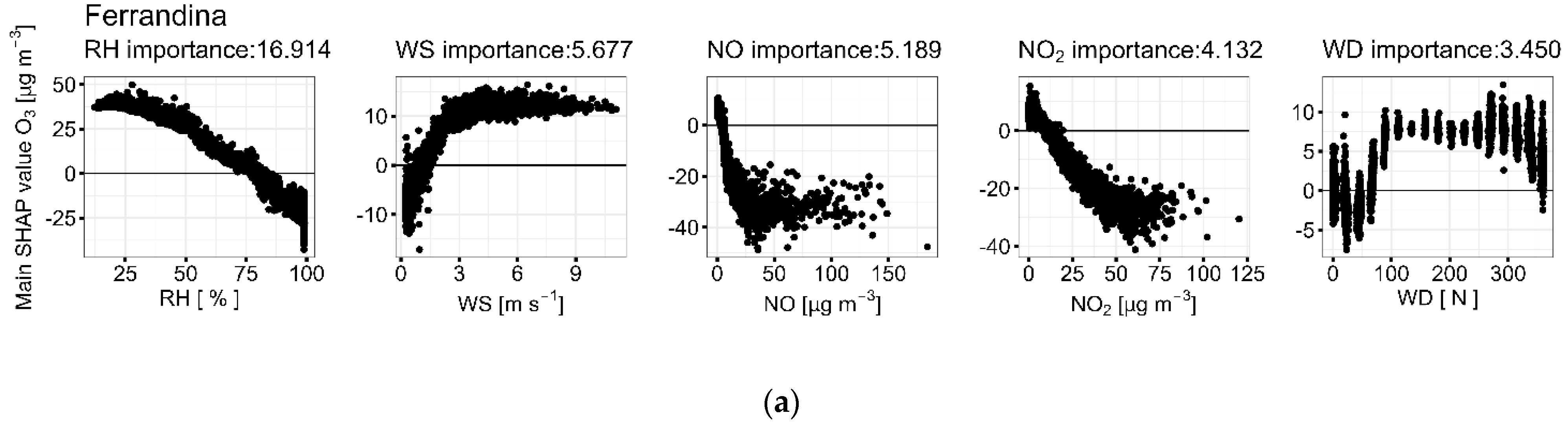
3.2.1. Meteorological Factors
3.2.2. Chemical Factors
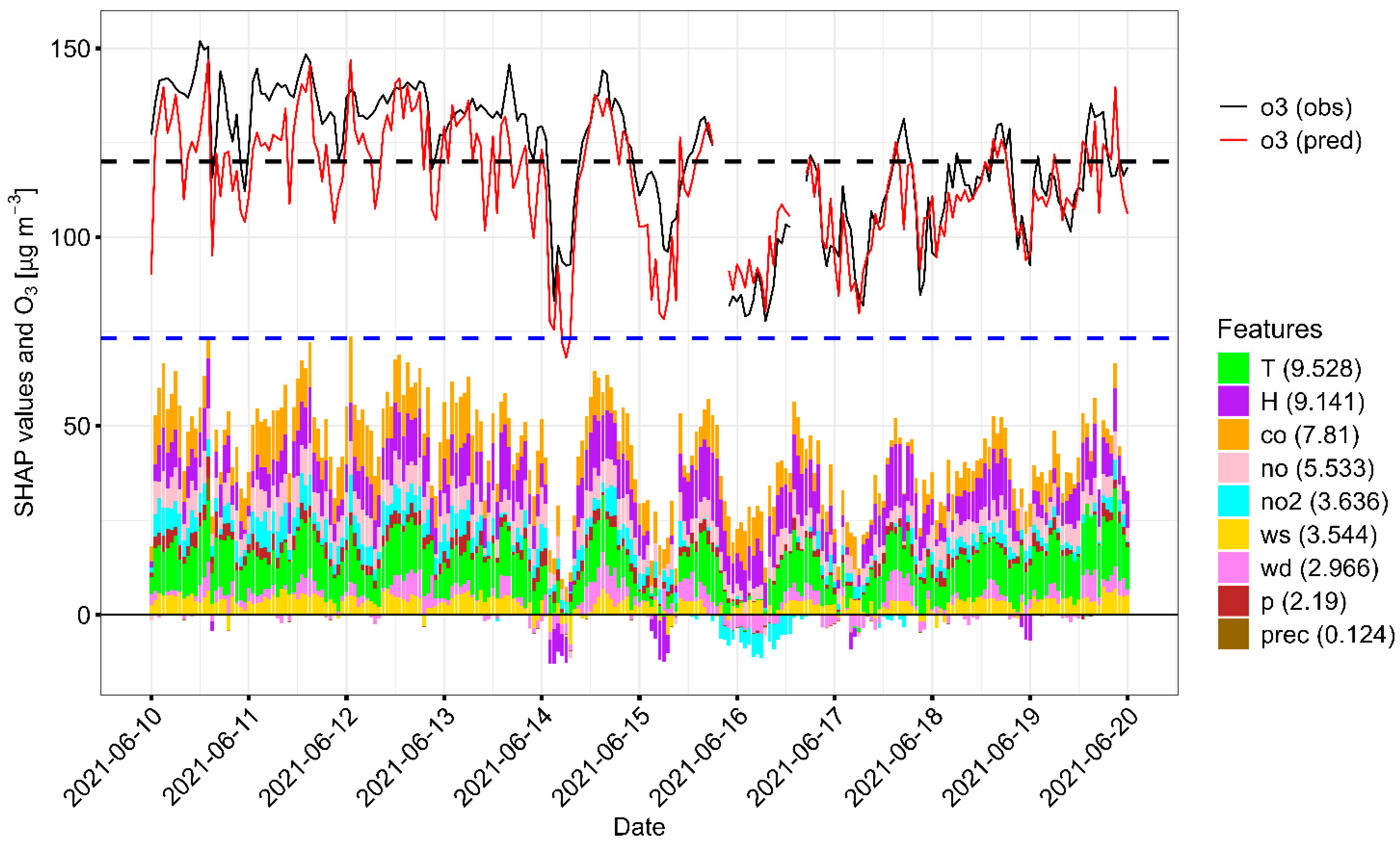
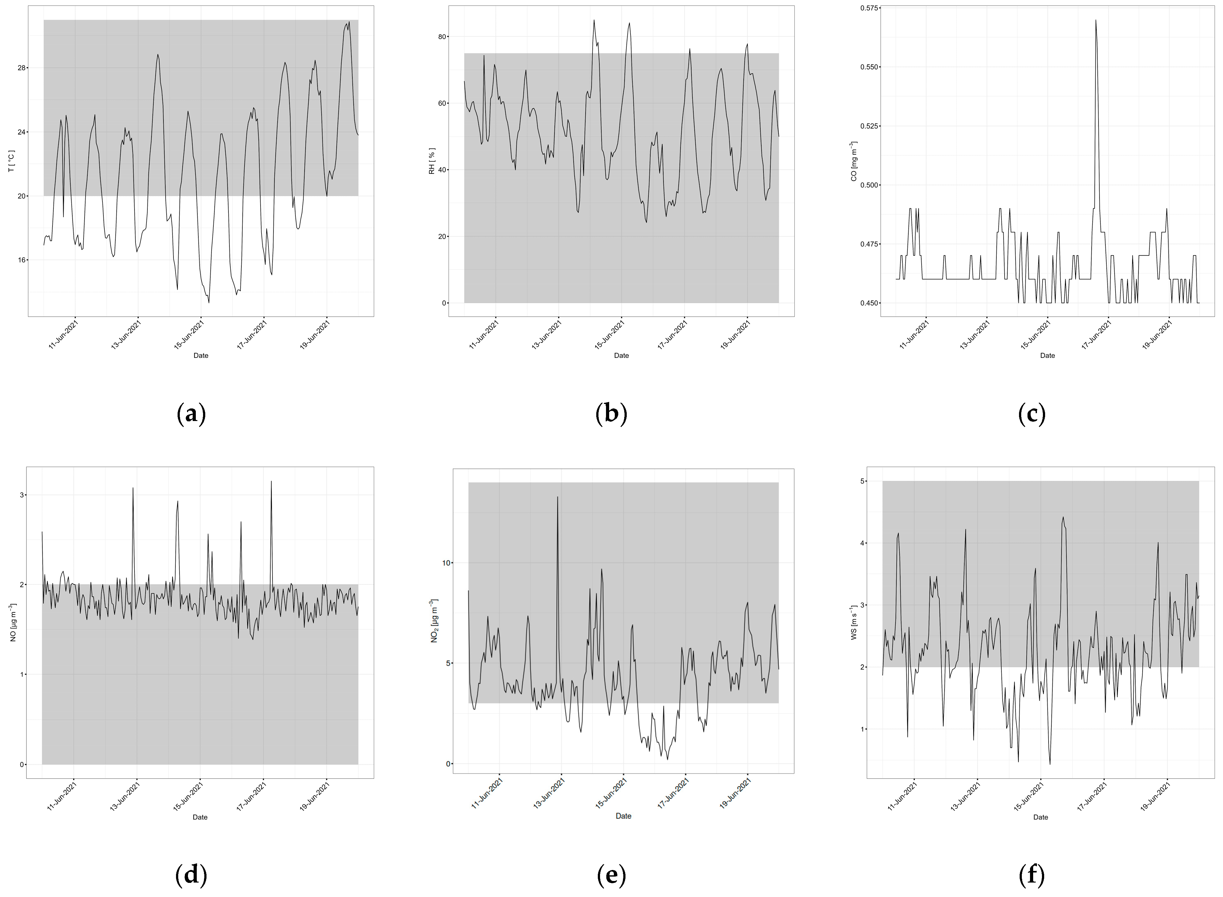
3.3. Contributing Factors to High Selected Pollution Event
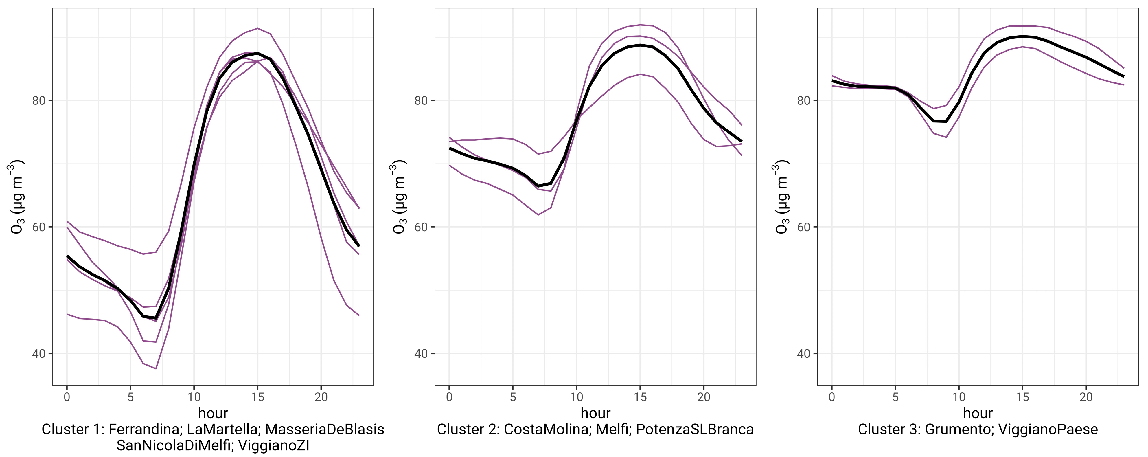
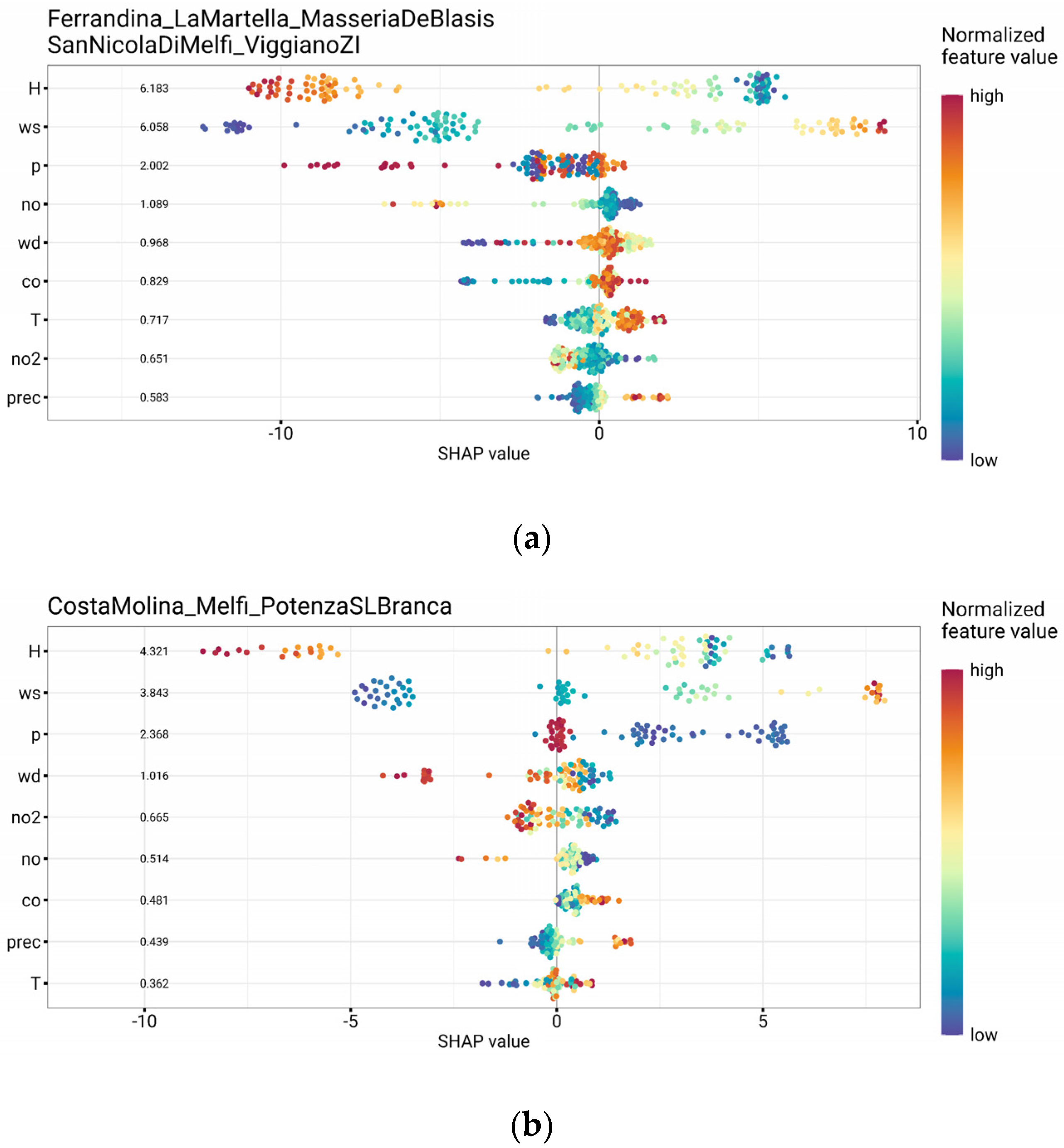
3.4. Contributing Factors to O3 Daily Pattern
4. Conclusions
Supplementary Materials
Author Contributions
Funding
Institutional Review Board Statement
Informed Consent Statement
Data Availability Statement
Acknowledgments
Conflicts of Interest
References
- Soares, A.R.; Silva, C. Review of Ground-Level Ozone Impact in Respiratory Health Deterioration for the Past Two Decades. Atmosphere 2022, 13, 434. [Google Scholar] [CrossRef]
- Donzelli, G.; Suarez-Varela, M.M. Tropospheric Ozone: A Critical Review of the Literature on Emissions, Exposure, and Health Effects. Atmosphere 2024, 15, 779. [Google Scholar] [CrossRef]
- Gao, P.; Wu, Y.; He, L.; Wang, L.; Fu, Y.; Chen, J.; Zhang, F.; Krafft, T.; Martens, P. Adverse Short-Term Effects of Ozone on Cardiovascular Mortalities Modified by Season and Temperature: A Time-Series Study. Front. Public Health 2023, 11, 1182337. [Google Scholar] [CrossRef]
- Grulke, N.E.; Heath, R.L. Ozone Effects on Plants in Natural Ecosystems. Plant Biol. 2020, 22, 12–37. [Google Scholar] [CrossRef] [PubMed]
- Friedrichová, R.; Karl, J.; Růžička, M.; Vyskočilová, A.; Martinec, M.; Veselý, M.; Škubník, J.; Svobodová Pavlíčková, V.; Rimpelová, S.; Kuchař, M. Determination of Ozone Concentration and Its Effect on Degradation of Materials. Trans. VŠB—Tech. Univ. Ostrav. Saf. Eng. Ser. 2022, 17, 14–25. [Google Scholar] [CrossRef]
- Pope, R.J.; Rap, A.; Pimlott, M.A.; Barret, B.; Le Flochmoen, E.; Kerridge, B.J.; Siddans, R.; Latter, B.G.; Ventress, L.J.; Boynard, A.; et al. Quantifying the Tropospheric Ozone Radiative Effect and Its Temporal Evolution in the Satellite Era. Atmos. Chem. Phys. 2024, 24, 3613–3626. [Google Scholar] [CrossRef]
- Dewan, S.; Lakhani, A. Tropospheric Ozone and Its Natural Precursors Impacted by Climatic Changes in Emission and Dynamics. Front. Environ. Sci. 2022, 10, 1007942. [Google Scholar] [CrossRef]
- Fu, T.M.; Tian, H. Climate Change Penalty to Ozone Air Quality: Review of Current Understandings and Knowledge Gaps. Curr. Pollut. Rep. 2019, 5, 159–171. [Google Scholar] [CrossRef]
- Hertig, E.; Jahn, S.; Kaspar-Ott, I. Future Local Ground-Level Ozone in the European Area From Statistical Downscaling Projections Considering Climate and Emission Changes. Earths Future 2023, 11, e2022EF003317. [Google Scholar] [CrossRef]
- Rezaei, R.; Güllü, G.; Ünal, A. Assessing the Impact of Climate Change on Summertime Tropospheric Ozone in the Eastern Mediterranean: Insights from Meteorological and Air Quality Modeling. Atmos. Environ. 2025, 344, 121036. [Google Scholar] [CrossRef]
- Chen, Z.Y.; Petetin, H.; Méndez Turrubiates, R.F.; Achebak, H.; Pérez García-Pando, C.; Ballester, J. Population Exposure to Multiple Air Pollutants and Its Compound Episodes in Europe. Nat. Commun. 2024, 15, 2094. [Google Scholar] [CrossRef] [PubMed]
- European Union. EU Directive (EU) 2024/2881 of the European Parliament and of the Council of 23 October 2024 on Ambient Air Quality and Cleaner Air for Europe (Recast). Off. J. Eur. Union. 2024. Available online: https://eur-lex.europa.eu/eli/dir/2024/2881/oj/eng (accessed on 1 October 2024).
- WHO. WHO Global Air Quality Guidelines. Particulate Matter (PM2.5 and PM10), Ozone, Nitrogen Dioxide, Sulfur Dioxide and Carbon Monoxide; World Health Organization: Geneva, Switzerland, 2021. [Google Scholar]
- EEA Europe’s Air Quality Status 2024. Available online: https://www.eea.europa.eu/publications/europes-air-quality-status-2024 (accessed on 19 November 2024).
- EEA Italy—Air Pollution Country Fact Sheet 2024. Available online: https://www.eea.europa.eu/en/topics/in-depth/air-pollution/air-pollution-country-fact-sheets-2024/italy-air-pollution-country-fact-sheet-2024 (accessed on 20 January 2025).
- SNPA. La Qualità Dell’aria in Italia Edizione 2023; Report Ambientali SNPA; SNPA: Rome, Italy, 2024; Volume 40, ISBN 9788844812072. [Google Scholar]
- Lyu, X.; Li, K.; Guo, H.; Morawska, L.; Zhou, B.; Zeren, Y.; Jiang, F.; Chen, C.; Goldstein, A.H.; Xu, X.; et al. A Synergistic Ozone-Climate Control to Address Emerging Ozone Pollution Challenges. One Earth 2023, 6, 964–977. [Google Scholar] [CrossRef]
- Jacob, D.J.; Winner, D.A. Effect of Climate Change on Air Quality. Atmos. Environ. 2009, 43, 51–63. [Google Scholar] [CrossRef]
- Mayer, M.; Schreier, S.F.; Spangl, W.; Staehle, C.; Trimmel, H.; Rieder, H.E. An Analysis of 30 Years of Surface Ozone Concentrations in Austria: Temporal Evolution, Changes in Precursor Emissions and Chemical Regimes, Temperature Dependence, and Lessons for the Future. Environ. Sci. Atmos. 2022, 2, 601–615. [Google Scholar] [CrossRef]
- Li, J.; Wang, Y.; Qu, H. Dependence of Summertime Surface Ozone on NOx and VOC Emissions Over the United States: Peak Time and Value. Geophys. Res. Lett. 2019, 46, 3540–3550. [Google Scholar] [CrossRef]
- Koplitz, S.; Simon, H.; Henderson, B.; Liljegren, J.; Tonnesen, G.; Whitehill, A.; Wells, B. Changes in Ozone Chemical Sensitivity in the United States from 2007 to 2016. ACS Environ. Au 2022, 2, 206–222. [Google Scholar] [CrossRef]
- Peng, Z.; Zhang, B.; Wang, D.; Niu, X.; Sun, J.; Xu, H.; Cao, J.; Shen, Z. Application of Machine Learning in Atmospheric Pollution Research: A State-of-Art Review. Sci. Total Environ. 2024, 910, 168588. [Google Scholar] [CrossRef]
- Masih, A. Machine Learning Algorithms in Air Quality Modeling. Glob. J. Environ. Sci. Manag. 2019, 5, 515–534. [Google Scholar]
- Méndez, M.; Merayo, M.G.; Núñez, M. Machine Learning Algorithms to Forecast Air Quality: A Survey. Artif. Intell. Rev. 2023, 56, 10031–10066. [Google Scholar] [CrossRef]
- Zheng, L.; Lin, R.; Wang, X.; Chen, W. The Development and Application of Machine Learning in Atmospheric Environment Studies. Remote Sens. 2021, 13, 4839. [Google Scholar] [CrossRef]
- Rybarczyk, Y.; Zalakeviciute, R. Machine Learning Approaches for Outdoor Air Quality Modelling: A Systematic Review. Appl. Sci. 2018, 8, 2570. [Google Scholar] [CrossRef]
- Li, W.; Ma, D.; Fu, J.; Qi, Y.; Shi, H.; Ni, T. A Quantitative Exploration of the Interactions and Synergistic Driving Mechanisms between Factors Affecting Regional Air Quality Based on Deep Learning. Atmos. Environ. 2023, 314, 120077. [Google Scholar] [CrossRef]
- Adadi, A.; Berrada, M. Peeking Inside the Black-Box: A Survey on Explainable Artificial Intelligence (XAI). IEEE Access 2018, 6, 52138–52160. [Google Scholar] [CrossRef]
- Chakraborty, S.; Misra, B.; Dey, N. Explainable Artificial Intelligence (XAI) for Air Quality Assessment. In Frontiers in Artificial Intelligence and Applications; IOS Press BV: Amsterdam, The Netherlands, 2024; Volume 383, pp. 333–341. [Google Scholar]
- Roscher, R.; Bohn, B.; Duarte, M.F.; Garcke, J. Explainable Machine Learning for Scientific Insights and Discoveries. IEEE Access 2020, 8, 42200–42216. [Google Scholar] [CrossRef]
- Oviedo, F.; Ferres, J.L.; Buonassisi, T.; Butler, K.T. Interpretable and Explainable Machine Learning for Materials Science and Chemistry. Acc. Mater. Res. 2022, 3, 597–607. [Google Scholar] [CrossRef]
- Lundberg, S.; Lee, S.-I. A Unified Approach to Interpreting Model Predictions. In Proceedings of the NIPS’17: Proceedings of the 31st International Conference on Neural Information Processing Systems, Long Beach, CA, USA, 4–9 December 2017. [Google Scholar]
- Lundberg, S.M.; Erion, G.; Chen, H.; DeGrave, A.; Prutkin, J.M.; Nair, B.; Katz, R.; Himmelfarb, J.; Bansal, N.; Lee, S.I. From Local Explanations to Global Understanding with Explainable AI for Trees. Nat. Mach. Intell. 2020, 2, 56–67. [Google Scholar] [CrossRef]
- Chen, Y.W.; Medya, S.; Chen, Y.C. Investigating Variable Importance in Ground-Level Ozone Formation with Supervised Learning. Atmos. Environ. 2022, 282, 119148. [Google Scholar] [CrossRef]
- Yao, T.; Lu, S.; Wang, Y.; Li, X.; Ye, H.; Duan, Y.; Fu, Q.; Li, J. Revealing the Drivers of Surface Ozone Pollution by Explainable Machine Learning and Satellite Observations in Hangzhou Bay, China. J. Clean. Prod. 2024, 440, 140938. [Google Scholar] [CrossRef]
- Zhang, L.; Wang, L.; Ji, D.; Xia, Z.; Nan, P.; Zhang, J.; Li, K.; Qi, B.; Du, R.; Sun, Y.; et al. Explainable Ensemble Machine Learning Revealing the Effect of Meteorology and Sources on Ozone Formation in Megacity Hangzhou, China. Sci. Total Environ. 2024, 922, 171295. [Google Scholar] [CrossRef]
- Ma, J.; Ding, Y.; Cheng, J.C.P.; Jiang, F.; Tan, Y.; Gan, V.J.L.; Wan, Z. Identification of High Impact Factors of Air Quality on a National Scale Using Big Data and Machine Learning Techniques. J. Clean. Prod. 2020, 244, 118955. [Google Scholar] [CrossRef]
- Bernier, C.; Wang, Y.; Estes, M.; Lei, R.; Jia, B.; Wang, S.C.; Sun, J. Clustering Surface Ozone Diurnal Cycles to Understand the Impact of Circulation Patterns in Houston, TX. J. Geophys. Res. Atmos. 2019, 124, 13457–13474. [Google Scholar] [CrossRef]
- Chen, Z.; Liu, R.; Wu, S.; Xu, J.; Wu, Y.; Qi, S. Diurnal Variation Characteristics and Meteorological Causes of Autumn Ozone in the Pearl River Delta, China. Sci. Total Environ. 2024, 908, 168469. [Google Scholar] [CrossRef]
- Stafoggia, M.; Oftedal, B.; Chen, J.; Rodopoulou, S.; Renzi, M.; Atkinson, R.W.; Bauwelinck, M.; Klompmaker, J.O.; Mehta, A.; Vienneau, D.; et al. Long-Term Exposure to Low Ambient Air Pollution Concentrations and Mortality among 28 Million People: Results from Seven Large European Cohorts within the ELAPSE Project. Lancet Planet Health 2022, 6, e9–e18. [Google Scholar] [CrossRef]
- Strak, M.; Weinmayr, G.; Rodopoulou, S.; Chen, J.; De Hoogh, K.; Andersen, Z.J.; Atkinson, R.; Bauwelinck, M.; Bekkevold, T.; Bellander, T.; et al. Long Term Exposure to Low Level Air Pollution and Mortality in Eight European Cohorts within the ELAPSE Project: Pooled Analysis. BMJ 2021, 374, n1904. [Google Scholar] [CrossRef]
- Liu, T.; Hong, Y.; Li, M.; Xu, L.; Chen, J.; Bian, Y.; Yang, C.; Dan, Y.; Zhang, Y.; Xue, L.; et al. Atmospheric Oxidation Capacity and Ozone Pollution Mechanism in a Coastal City of Southeastern China: Analysis of a Typical Photochemical Episode by an Observation-Based Model. Atmos. Chem. Phys. 2022, 22, 2173–2190. [Google Scholar] [CrossRef]
- D’Amico, F.; Gullì, D.; Lo Feudo, T.; Ammoscato, I.; Avolio, E.; De Pino, M.; Cristofanelli, P.; Busetto, M.; Malacaria, L.; Parise, D.; et al. Cyclic and Multi-Year Characterization of Surface Ozone at the WMO/GAW Coastal Station of Lamezia Terme (Calabria, Southern Italy): Implications for Local Environment, Cultural Heritage, and Human Health. Environments 2024, 11, 227. [Google Scholar] [CrossRef]
- Coluzzi, R.; D’emilio, M.; Imbrenda, V.; Giorgio, G.A.; Lanfredi, M.; Macchiato, M.; Ragosta, M.; Simoniello, T.; Telesca, V. Investigating Climate Variability and Long-Term Vegetation Activity across Heterogeneous Basilicata Agroecosystems. Geomat. Nat. Hazards Risk 2019, 10, 168–180. [Google Scholar] [CrossRef]
- Blanco, A.; De Tomasi, F.; Filippo, E.; Manno, D.; Perrone, M.R.; Serra, A.; Tafuro, A.M.; Tepore, A. Characterization of African Dust over Southern Italy. Atmos. Chem. Phys. 2003, 3, 2147–2159. [Google Scholar] [CrossRef]
- Wang, Q.; Gu, J.; Wang, X. The Impact of Sahara Dust on Air Quality and Public Health in European Countries. Atmos. Environ. 2020, 241, 117771. [Google Scholar] [CrossRef]
- Sicard, P.; De Marco, A.; Troussier, F.; Renou, C.; Vas, N.; Paoletti, E. Decrease in Surface Ozone Concentrations at Mediterranean Remote Sites and Increase in the Cities. Atmos. Environ. 2013, 79, 705–715. [Google Scholar] [CrossRef]
- Cristofanelli, P.; Bonasoni, P. Background Ozone in the Southern Europe and Mediterranean Area: Influence of the Transport Processes. Environ. Pollut. 2009, 157, 1399–1406. [Google Scholar] [CrossRef] [PubMed]
- ARPA Basilicata. Raccolta Annuale dei Dati Ambientali, Anno 2022; ARPA Basilicata: Basilicata, Italy, 2023; Volume 1. [Google Scholar]
- Chen, T.; Guestrin, C. XGBoost: A Scalable Tree Boosting System. In Proceedings of the ACM SIGKDD International Conference on Knowledge Discovery and Data Mining; Association for Computing Machinery, New York, NY, USA, 13–17 August 2016; pp. 785–794. [Google Scholar]
- Molnar, C. Interpretable Machine Learning. A Guide for Making Black Box Models Explainable; Leanpub: Victoria, BC, Canada, 2021. [Google Scholar]
- Ponce-Bobadilla, A.V.; Schmitt, V.; Maier, C.S.; Mensing, S.; Stodtmann, S. Practical Guide to SHAP Analysis: Explaining Supervised Machine Learning Model Predictions in Drug Development. Clin. Transl. Sci. 2024, 17, e70056. [Google Scholar] [CrossRef]
- Hartigan, J.A.; Wong, M.A. Algorithm AS 136: A K-Means Clustering Algorithm. J. R. Stat. Soc. Ser. C Appl. Stat. 1979, 28, 100–108. [Google Scholar] [CrossRef]
- Govender, P.; Sivakumar, V. Application of K-Means and Hierarchical Clustering Techniques for Analysis of Air Pollution: A Review (1980–2019). Atmos. Pollut. Res. 2020, 11, 40–56. [Google Scholar] [CrossRef]
- Kang, Y.; Choi, H.; Im, J.; Park, S.; Shin, M.; Song, C.K.; Kim, S. Estimation of Surface-Level NO2 and O3 Concentrations Using TROPOMI Data and Machine Learning over East Asia. Environ. Pollut. 2021, 288, 117711. [Google Scholar] [CrossRef]
- Luo, Z.; Lu, P.; Chen, Z.; Liu, R. Ozone Concentration Estimation and Meteorological Impact Quantification in the Beijing-Tianjin-Hebei Region Based on Machine Learning Models. Earth Space Sci. 2024, 11, e2023EA003346. [Google Scholar] [CrossRef]
- Gagliardi, R.V.; Andenna, C. A Machine Learning Approach to Investigate the Surface Ozone Behavior. Atmosphere 2020, 11, 1173. [Google Scholar] [CrossRef]
- Ordóñez, C.; Garrido-Perez, J.M.; García-Herrera, R. Early Spring Near-Surface Ozone in Europe during the COVID-19 Shutdown: Meteorological Effects Outweigh Emission Changes. Sci. Total Environ. 2020, 747, 141322. [Google Scholar] [CrossRef]
- Ni, J.; Jin, J.; Wang, Y.; Li, B.; Wu, Q.; Chen, Y.; Du, S.; Li, Y.; He, C. Surface Ozone in Global Cities: A Synthesis of Basic Features, Exposure Risk, and Leading Meteorological Driving Factors. Geogr. Sustain. 2024, 5, 64–76. [Google Scholar] [CrossRef]
- Li, M.; Yu, S.; Chen, X.; Li, Z.; Zhang, Y.; Wang, L.; Liu, W.; Li, P.; Lichtfouse, E.; Rosenfeld, D.; et al. Large Scale Control of Surface Ozone by Relative Humidity Observed during Warm Seasons in China. Environ. Chem. Lett. 2021, 19, 3981–3989. [Google Scholar] [CrossRef]
- Laban, T.L.; Van Zyl, P.G.; Beukes, J.P.; Mikkonen, S.; Santana, L.; Josipovic, M.; Vakkari, V.; Thompson, A.M.; Kulmala, M.; Laakso, L. Statistical Analysis of Factors Driving Surface Ozone Variability over Continental South Africa. J. Integr. Environ. Sci. 2020, 17, 1–28. [Google Scholar] [CrossRef]
- Camalier, L.; Cox, W.; Dolwick, P. The Effects of Meteorology on Ozone in Urban Areas and Their Use in Assessing Ozone Trends. Atmos. Environ. 2007, 41, 7127–7137. [Google Scholar] [CrossRef]
- Cheng, N.; Jing, D.; Gu, Z.; Cai, X.; Shi, Z.; Li, S.; Chen, L.; Li, W.; Wang, Q. Observation-Based Ozone Formation Rules by Gradient Boosting Decision Trees Model in Typical Chemical Industrial Parks. Atmosphere 2024, 15, 600. [Google Scholar] [CrossRef]
- Borhani, F.; Shafiepour Motlagh, M.; Stohl, A.; Rashidi, Y.; Ehsani, A.H. Tropospheric Ozone in Tehran, Iran, during the Last 20 Years. Environ. Geochem. Health 2022, 44, 3615–3637. [Google Scholar] [CrossRef]
- Han, H.; Liu, J.; Shu, L.; Wang, T.; Yuan, H. Local and Synoptic Meteorological Influences on Daily Variability in Summertime Surface Ozone in Eastern China. Atmos. Chem. Phys. 2020, 20, 203–222. [Google Scholar] [CrossRef]
- Kavassalis, S.C.; Murphy, J.G. Understanding Ozone-Meteorology Correlations: A Role for Dry Deposition. Geophys. Res. Lett. 2017, 44, 2922–2931. [Google Scholar] [CrossRef]
- Liao, Z.; Pan, Y.; Ma, P.; Jia, X.; Cheng, Z.; Wang, Q.; Dou, Y.; Zhao, X.; Zhang, J.; Quan, J. Meteorological and Chemical Controls on Surface Ozone Diurnal Variability in Beijing: A Clustering-Based Perspective. Atmos. Environ. 2023, 295, 119566. [Google Scholar] [CrossRef]
- Cheng, Y.; Huang, X.F.; Peng, Y.; Tang, M.X.; Zhu, B.; Xia, S.Y.; He, L.Y. A Novel Machine Learning Method for Evaluating the Impact of Emission Sources on Ozone Formation. Environ. Pollut. 2023, 316, 120685. [Google Scholar] [CrossRef] [PubMed]
- Zhang, C.; Xie, Y.; Shao, M.; Wang, Q. Application of Machine Learning to Analyze Ozone Sensitivity to Influencing Factors: A Case Study in Nanjing, China. Sci. Total Environ. 2024, 929, 172544. [Google Scholar] [CrossRef]
- Nguyen, D.H.; Lin, C.; Vu, C.T.; Cheruiyot, N.K.; Nguyen, M.K.; Le, T.H.; Lukkhasorn, W.; Vo, T.D.H.; Bui, X.T. Tropospheric Ozone and NOx: A Review of Worldwide Variation and Meteorological Influences. Environ. Technol. Innov. 2022, 28, 102809. [Google Scholar] [CrossRef]
- Bi, Z.; Ye, Z.; He, C.; Li, Y. Analysis of the Meteorological Factors Affecting the Short-Term Increase in O3 Concentrations in Nine Global Cities during COVID-19. Atmos. Pollut. Res. 2022, 13, 101523. [Google Scholar] [CrossRef] [PubMed]
- Lee, H.J.; Chang, L.S.; Jaffe, D.A.; Bak, J.; Liu, X.; Abad, G.G.; Jo, H.Y.; Jo, Y.J.; Lee, J.B.; Kim, C.H. Ozone Continues to Increase in East Asia despite Decreasing NO2: Causes and Abatements. Remote Sens. 2021, 13, 2177. [Google Scholar] [CrossRef]
- Chen, J.; Shen, H.; Li, T.; Peng, X.; Cheng, H.; Ma, C. Temporal and Spatial Features of the Correlation between PM2.5 and O3 Concentrations in China. Int. J. Environ. Res. Public Health 2019, 16, 4824. [Google Scholar] [CrossRef]
- Wang, J.; Dong, J.; Guo, J.; Cai, P.; Li, R.; Zhang, X.; Xu, Q.; Song, X. Understanding Temporal Patterns and Determinants of Ground-Level Ozone. Atmosphere 2023, 14, 604. [Google Scholar] [CrossRef]
- Agathokleous, S.; Saitanis, C.J.; Savvides, C.; Sicard, P.; Agathokleous, E.; De Marco, A. Spatiotemporal Variations of Ozone Exposure and Its Risks to Vegetation and Human Health in Cyprus: An Analysis across a Gradient of Altitudes. J. For. Res. 2023, 34, 579–594. [Google Scholar] [CrossRef]
- An, C.; Li, H.; Ji, Y.; Chu, W.; Yan, X.; Chai, F. A Review on Nocturnal Surface Ozone Enhancement: Characterization, Formation Causes, and Atmospheric Chemical Effects. Sci. Total Environ. 2024, 921, 170731. [Google Scholar] [CrossRef]
- Wang, K.; Xie, F.; Sulaymon, I.D.; Gong, K.; Li, N.; Li, J.; Hu, J. Understanding the Nocturnal Ozone Increase in Nanjing, China: Insights from Observations and Numerical Simulations. Sci. Total Environ. 2023, 859, 160211. [Google Scholar] [CrossRef]
- He, G.; He, C.; Wang, H.; Lu, X.; Pei, C.; Qiu, X.; Liu, C.; Wang, Y.; Liu, N.; Zhang, J.; et al. Nighttime Ozone in the Lower Boundary Layer: Insights from 3-Year Tower-Based Measurements in South China and Regional Air Quality Modeling. Atmos. Chem. Phys. 2023, 23, 13107–13124. [Google Scholar] [CrossRef]


| Site | ID | Station Type, Area | Latitude N | Longitude E | Altitude (m a.s.l.) |
|---|---|---|---|---|---|
| Costa Molina | CM | Industrial, rural | 15°57′17″,2 | 40°18′56″,2 | 690 |
| Ferrandina | FE | Industrial, rural | 16°29′46″,4 | 40°29′09″,0 | 63 |
| Grumento | GR | Industrial, sub urban | 15°53′29″,1 | 40°17′18″,2 | 735 |
| La Martella | LM | Industrial, sub urban | 16°32′49″,7 | 40°41′11″,9 | 245 |
| Masseria De Blasis | MdB | Industrial, rural | 15°52′02″,5 | 40°19′27″,2 | 603 |
| Melfi | ME | Industrial, sub urban | 15°38′23″,9 | 40°59′02″,8 | 561 |
| Potenza SL Branca | PZB | Industrial, sub urban | 15°52′22″,4 | 40°38′38″,0 | 720 |
| San Nicola Di Melfi | SNM | Industrial, rural | 15°43′21″,9 | 41°04′01″,4 | 187 |
| Viggiano Paese | VP | Industrial, rural | 15°54′02″,5 | 40°20′05″,5 | 820 |
| Viggiano ZI | VZI | Industrial, rural | 15°54′16″,4 | 40°18′50″,6 | 604 |
| Site | RH [%] | T [°C] | ws [m/s] | NO2 [μg/m3] | NO [μg/m3] |
|---|---|---|---|---|---|
| Most favorable feature conditions to O3 accumulation | <75 | >20 | >2 2 ÷ 5 * | <5 >3 * | <2 |
| CM | <75 | >17 | >2 | <4 | <2 |
| FE | <80 | ** | >1 | <10 | <4 |
| GR | <73 | >15 | >2 | <5 | <2 |
| LM | <77 | >20 | ** | <8 | ** |
| MdB | <85 | >20 | >2 | <5 | ** |
| ME | <72 | >17 | 2 ÷ 5 | >3 ** | <2 |
| PZB | <75 | >20 | >1 | <8 | ** |
| SNM | <73 | >17 | >2 | <13 | <5 |
| VP | <60 | >17 | >2 | <4 | ** |
| VZI | <78 | >15 | >1 | <6 | <4 |
Disclaimer/Publisher’s Note: The statements, opinions and data contained in all publications are solely those of the individual author(s) and contributor(s) and not of MDPI and/or the editor(s). MDPI and/or the editor(s) disclaim responsibility for any injury to people or property resulting from any ideas, methods, instructions or products referred to in the content. |
© 2025 by the authors. Licensee MDPI, Basel, Switzerland. This article is an open access article distributed under the terms and conditions of the Creative Commons Attribution (CC BY) license (https://creativecommons.org/licenses/by/4.0/).
Share and Cite
Gagliardi, R.V.; Andenna, C. Exploring the Influencing Factors of Surface Ozone Variability by Explainable Machine Learning: A Case Study in the Basilicata Region (Southern Italy). Atmosphere 2025, 16, 491. https://doi.org/10.3390/atmos16050491
Gagliardi RV, Andenna C. Exploring the Influencing Factors of Surface Ozone Variability by Explainable Machine Learning: A Case Study in the Basilicata Region (Southern Italy). Atmosphere. 2025; 16(5):491. https://doi.org/10.3390/atmos16050491
Chicago/Turabian StyleGagliardi, Roberta Valentina, and Claudio Andenna. 2025. "Exploring the Influencing Factors of Surface Ozone Variability by Explainable Machine Learning: A Case Study in the Basilicata Region (Southern Italy)" Atmosphere 16, no. 5: 491. https://doi.org/10.3390/atmos16050491
APA StyleGagliardi, R. V., & Andenna, C. (2025). Exploring the Influencing Factors of Surface Ozone Variability by Explainable Machine Learning: A Case Study in the Basilicata Region (Southern Italy). Atmosphere, 16(5), 491. https://doi.org/10.3390/atmos16050491