Abstract
In an attempt to reconciliate air-sea momentum flux estimates derived from open sea observations, from large eddy simulation output fields, and from wind-wave tank measurements, a series of dedicated experiments were conducted in the wind-wave tank of the Large Air-Sea Facility of Marseille, France. The turbulent friction velocity, upon which the momentum flux depends, was estimated from wind measurements by applying four classical methods including the eddy-covariance method and the inertial-dissipation method. The collected data were used to investigate some characteristics of the wave-influenced boundary layer that were predicted by previous simulations, and to quantify a wave-dependent term of the turbulent kinetic energy equation, the so-called imbalance term . Our results show that the turbulent stress decreases toward lower heights where the effect of waves is large, as in the simulations, and that is in the range 0.3 to 0.7, which is comparable to the value found with open sea data (0.4). These preliminary results have to be confirmed with wave-following probes, because the estimated eddy-covariance flux slightly varied with height, thus it could not be strictly considered to be equal to a constant total flux.
1. Introduction
1.1. Context
Wind-generated waves significantly modify the marine atmospheric boundary layer (MABL) and the atmospheric turbulence above them. They function as roughness elements enhancing turbulence and surface fluxes (momentum, heat, and moisture) between atmosphere and ocean. Air-sea momentum exchanges are expressed through the wind shear stress . They are responsible for the wave generation and growth [1], as well as for the development and intensity changes of tropical cyclones [2].
Therefore, a comprehensive representation of wind stress is necessary for improving weather forecasting and ocean circulation models, as well as for predicting extreme events such as tropical cyclones and rogue waves. The accuracy of numerical models largely relies on the accuracy of the parameterization used for the shear stress. Indeed, the stress depends on variables, such as wind speed, for example, but at scales that are not resolved by operational models.
The Monin-Obukhov Similarity Theory (MOST hereafter) is widely used to describe turbulent exchanges in the atmospheric boundary layer (ABL) since the mid-20th century [3,4]. This has been possible after the validation of the statistical formulas derived by MO theory by the pioneering terrestrial field experiments of 1960s and 1970s, such as the 1968 Kansas and the 1973 Minnesota ones [5,6,7].
Marine atmospheric boundary layer (MABL) modeling requires an adjusted approach employing MO similarity theory and additional scaling parameters to describe the momentum exchange due to surface waves. Unlike terrestrial surface roughness such as vegetation and buildings, which have constant or slowly varying height, wind-generated waves act as dynamic surface roughness elements directly generated by the air-sea momentum exchange itself. They also affect momentum exchange in the MABL by generating sea spray during waves’ breaking [8,9], particularly under strong wind conditions [10]. Thus, modeling of air-sea exchanges requires to consider scaling parameters related to wave presence in addition to the classic mechanical and thermal forcing of turbulent exchanges in atmospheric boundary layer (ABL) [11,12]. The wave-induced modulations of the MABL turbulence were firstly identified by [13], followed by [14]. Further details on the specificities of MABL modeling compared to ABL modeling over land can be found in the Section 1.2 and Section 1.3 below, and in the work of [15].
Parametrizations of wind shear stress in the MABL may arise from various sources, theories, experimental data, simulations, or a combination of the above. Some of the most prominent approaches have incorporated the effect of surface waves by refining the expression of roughness length, , as seen in the historic works of [16,17], and the more recent work of [18]. The latter presents the improved COARE algorithm, which includes a roughness length parametrization divided into a smooth component, , and a rough component, , depending on the wind stress in the form of surface gravity waves. In order to define , the authors compare wind-dependent and wave-dependent formulations of , ultimately concluding that a wind-dependent formulation is sufficient at open-ocean conditions when there are only wind-generated waves and not swell.
At one point these parameterizations need to be validated by in situ data, in order to be qualified. Unfortunately, estimating the stress at sea is a demanding task, because the platforms generally disturb the measurements (airflow distortion, radiation effects, reflection waves, or height displacement) and they have multiple other limitations. For example, fixed platforms may provide valuable long-term datasets but they are usually not in open sea conditions being affected by orographic effects and representing very specific coastal environments. Some examples are the Martha’s Vineyard platform of Woods Hole Oceanographic Institution (WHOI) [19] and the Black Sea platform [20]. Towed platforms, as pioneered by [21], have been important for measuring small-scaling variations of SST and SSS. However, their position within the disturbed atmospheric wake limits their ability to measure waves and atmospheric turbulence measurements.
In the recent years, a great progress in computing flux estimates has been made due to the development of ship-mounted systems and wave-following platforms (e.g., [22,23,24,25,26,27,28,29]). However, these platforms have their own limitations. They are not Eulerian and have their own vertical motion (buoys that follow the surface and heave on Research Vessels, referred to as R/Vs hereafter) requiring the application of a platform-motion correction algorithm before using wind measurements. Additionally, instruments cannot always be placed close to the water surface due to the risk of salt contamination. For further details on the available air-sea exchanges platforms, one can refer to the introduction of the paper [22].
In order to elucidate biases and other uncertainties associated with the estimation of stress and of its subsequent parameterization from open ocean data, it is helpful to perform experiments in a wind-wave tunnel (WWT), in which the conditions of the experiments are controlled. First works on WWT tunnels were using Pitot-static tubes and hot-film probes, to measure mean wind velocity and wind velocity fluctuations, respectively [30,31]. However, recent studies employ advanced wind-measuring systems that allow high-resolution measurements of wind fluctuations and enable the determination of turbulent Reynolds stress through the calculation of the cross-correlation term, . Calculating requires high temporal resolution wind measurements in two directions, as achieved using the X-wire probe in our case. Optical methods, such as the combined particle image velocimetry (PIV) and laser induced fluorescence (LIF) system, as used by [32], allow spatial averaging of the flow leading to the calculation of the less known dispersive term of Reynolds stress. However, these methods are costly and less accessible compared to constant temperature anemometry (CTA) probes used here. Regarding the limitations of WWT in our case, they are mostly due to the shorter waves compared to those in the open ocean.
The present article is an attempt to reconciliate open sea data (OCARINA wave following platform [22], or B19 hereafter) with WWT data, regarding the estimation of the wind shear stress (in units of N m−2) as transferred from air to sea.
The following presents a preliminary comparison between the B19 multi-campaign dataset collected in the open ocean, and data from a dedicated series of WWT experiments conducted from April to July 2022, focusing on the precise determination of momentum fluxes.
1.2. The Surface Boundary Layer
Until the late nineties, the lower part of the atmospheric boundary layer from 1 mm to 10 m, was referred to as constant-flux Surface Boundary Layer (SBL hereafter), in which the momentum transferred from air to the surface was identified as a shear stress at turbulent scales [33]. This view was inherited from over-land studies, and earlier, to the study of wall-bounded flows. The properties of stress could be deduced from the application of a two-scale Reynolds decomposition of the flow governing variables such as the wind vector to the Navier-Stokes equation expressed in a two-dimensional referential where the x-axis was aligned with the mean -or synoptic- wind vector (at a timescale that encompasses the integral scale of turbulence as a first approximation), and the z-axis was directed upward. Along the x-axis, the decomposition is written as , where is the turbulent fluctuation of the wind, the average of which is zero. The resulting expression of the shear stress is written as,
where can be neglected at heights larger than a fraction of a millimeter above the surface, which are not investigated here, where the covariance term is the so-called turbulent momentum flux associated to its counterpart in terms of stress , and where is the density of air, in kg m−3.
The two-scale decomposition described above is completed by similarity arguments, based on MOST. According to this theory, one may indifferently use the stress , the momentum flux, or a new velocity scale so-called friction velocity (in m s−1) that is defined as,
A helpful result of the MOST is that it gives one the shape of the mean wind profile , which has the following form,
where is the von Karman constant that is equal to 0.4, z is the measuring height, and is a second new variable referred to as turbulent roughness length of the surface.
For comparison, note that the so-called Eddy-Covariance Method, or EC Method hereafter, is the direct application of Equation (1), which may be rewritten as,
Unfortunately, the experimentalists realized that the value of over the Sea depended on a complex way on several variables such as the wind speed or certain wave characteristics [34,35].
1.3. The Wave-Induced Boundary Layer
A three-scale decomposition specific to the Marine SBL was suggested by several authors as [36]. It is written as , where is a wind component associated with the presence of waves, which is often referred to as wind undulation. Although it is more complex than a two-scale decomposition, it sets the basis of the modern view of air-sea momentum exchanges in which the shear stress is now the sum of two terms, one of which () depends on waves,
where was again neglected. Among the existing theoretical and simulations results based on the three-scale decomposition, the Large Eddy Simulation (LES) of [37] (or HS15 hereafter) is -to our knowledge- the most informative about the profiles of wind velocity, wind shear and shear stress close to sinusoidal waves. It is also a first step to achieve simulations in conditions of more complex sea states in the future.
Regarding the issue addressed in the present manuscript, HS15 made clear to the scientific community several breakthrough and helpful results, the first of which being the commonly acknowledged existence of a layer of atmosphere where the influence of waves was prominent, the so-called Wave-influenced Boundary Layer (WBL).
The reader should note that according to HS15, is constant along the vertical throughout the WBL down to the surface. Their simulations show that the decreases as one gets deeper in the WBL, and becomes zero at the water surface.
HS15 made also clear that the stress estimated with instruments onboard a wave-following platform by applying the EC Method would be , whereas the application of an alternate method so-called Inertial-Dissipation Method (or ID Method hereafter) [15] gives an estimate of , if our understanding is correct. This will be further discussed in the next section as these points are central to the present study.
Although HS15 did an unprecedented effort to document the WBL, their study expectedly has limitations that are mainly inherent to the facts that first, idealized sine wave conditions are rarely encountered in the open sea. Next, their vertical 2D simulations might not reflect what could be found with a full 3D view of the problem. Last, they do not propose any parameterization of .
Nevertheless, the connection of the HS15 simulations to observations is now required to better characterize the WBL in cases of swell, of wind-driven waves, and of mixed regimes. In addition, it is feasible to verify the shape of the vertical profile of the stress, component per component, with a WWT experiment.
Although there are unfortunately little chances to reach a realistic parameterization of from these preliminary cross-comparisons, we are convinced that doing so is a step forward to the right direction to achieve this goal.
1.4. Imbalance Term in the TKE Equation
Not only the comparison between WWT data to HS15 simulation may give one confidence in the HS15 description of the WBL and of the stress and wind profiles, as suggested in Section 1.3, but it also inspired us to elucidate a still debated question regarding the estimation of with the ID Method for open sea data.
The ID Method has the tremendous advantage of making the estimates of independent from the platform motion, whereas motion strongly limits the application of EC Method in which has to be corrected from the vertical platform velocity [38].
The ID Method is based on the second-order [39] relation, which, after application of the Taylor frozen turbulence hypothesis, so as to convert wave wavenumber into wave frequency, is written as,
where is the dissipation rate of turbulence in m2 s−3, f is the frequency in Hz, is the power spectral density (PSD) function of u in m2 s−2 Hz−1, and is the Kolmogorov constant that is equal to 0.55. Consequently, the calculation of the PSD of u in the inertial sub-range (e.g., B19) gives an estimate of .
In a second step, the diagnostic equation for the Turbulent Kinetic Energy (TKE hereafter), the definition of which is , with assumptions of steady and non-buoyant (neutral) flow and of horizontal homogeneity,
where p is the static pressure, in Pa. In a first step, let us assume that the second and the third term in the left hand side of Equation (7) are neglected. After applying the MOST to Equation (7), the expression of is readily obtained, which is written as,
Unfortunately, when B19 compared to and to for six sea experiments, they found that the above mentioned three estimates differed from each other, even in mean conditions, i.e., swell and moderate wind speed. The agreement was obtained by adding a constant term on the order of 0.4 to Equation (7), which may be rewritten as,
where refers to an estimate of in which is accounted for. Clearly, accounts for the second and third term of Equation (7).
Experimentally, few is known about the pressure term, i.e., the third term of Equation (7), because it is simply not measured as no reliable instrument exists for moving platforms, to the best of our knowledge. It explains why it is generally neglected.
Interestingly, B19 noticed that if was set to zero, then the estimates of were underestimated in comparison to or even to , which supports the hypothesis that would correspond to pure turbulence. In addition, this would comply with the HS15 results according to which the turbulent stress decreases in the WBL, where the OCARINA wave-following platform used in B19 actually evolves. This will be detailed in Section 2.1.
In the following paragraph, for the sake of completeness, we feel compelled to give the reader more context about a twenty-year or so old lasting polemic about the requirement of in the ID calculation.
In experiments performed onboard R/Vs, the turbulence measurement instruments are mounted on top of a mast that is located at the bow. Several authors such as [40] showed that with this setup, was required to correct estimates, where z/L is the so-called Monin-Obukhov ratio that quantifies the dynamic stability of the SBL, which appears in an additional so-called buyancy production/destruction term, intentionnally omitted from Equation (9), because it is not central to our study. However, there was a controversy on the need to take this term into account to estimate , in favor of a modification of [41]. This was later challenged by [42], who confirmed [40] results. It has to be noted that unexpectedly, a recent revisit of [42] data suggests that was actually negligible for this experiment, which reopens the question (manuscript in preparation).
Nevertheless, the difference between the height of the measuring instruments on ship (between 7 m and 18 m depending on the length of the ship) and on low-profile buoys (<2 m) partly explains here the differences between the results: data obtained with low-profile platforms are carried out in the WBL, whereas on R/Vs the measurements are collected far above it. Thus, even if z/L plays a role in the TKE equation, B19 clearly showed that it was of secondary order compared to the effect of the pressure term.
With their constant , B19 could largely reconciliate EC, ID and MOST estimated of , thus they found a way to adapt ID Method based on a two-scale decomposition to get a total stress. In earlier studies, the pressure term usually represented only the return to isotropy [43]. The B19 results suggested that in the WBL this term would be rather related to waves, which is also clearly predicted by the simulations of HS15.
The fact that HS15 applies a three-scale decomposition implies that there is also a normal stress (the form drag) exerted by the wind on the upwind face of the waves plus a tangential stress due to the waves, the wave-induced stress. This illustrates the complexity of the process here in focus.
Overall, there is a strong need to estimate in the WBL. A direct benefit of it would be a way to correct estimates, to ultimately obtain the total stress, which is the quantity that one wants to force an ocean model for example.
To verify this, it would be helpful to first assess the ratio , or more explicitly as a function of height, in a controlled environment for different heights, and in various wave conditions. Next, estimates of would also help. Indeed, in the open ocean, the estimates are drowned in a lot of noise, despite the use of platforms like OCARINA already greatly helped to decrease the uncertainties compared to measurements performed on R/Vs.
Note that with MOST, can be easily deduced from estimates by applying Equation (3). In addition, the same relation may be used for estimating from estimates.
1.5. Summary and Plan of the Proposed Study
Our primary objective was to elucidate and the vertical profile of and of its components and . Our technique was to maximize our confidence in the results by crossing information from three sources, namely simulations, open sea data (B19), and WWT data. Secondary objectives would be to improve our definition of the WBL, specifically its height as a function of wind velocity in WWT data.
The study is organized as follows. The existing B19 open sea data are briefly presented in Section 2.1 for easing the reading of the manuscript and the recent WWT experiment are described in Section 2.2. Next, the WWT data are analyzed for the mean and turbulent flows, successively, in Section 3.1. In Section 3.2, estimations of the different stresses and the way to obtain them are presented, and the subsequent estimates of are compared to open sea data. A discussion follows.
2. Materials and Methods
2.1. Open Sea Data
Friction velocity at the air-sea interface was estimated by data collected during six experiments from 2011 to 2017 in four different regions with a low-profile dedicated wave-following platform so-called OCARINA, shown in Figure 1. The OCARINA platform is a 2-m-long trimaran boat, motorized with a propeller and equipped with a remote control system. Five main measuring sensors are mounted on the platform: the Kipp & Zonen CNR4 for radiation fluxes, the Movella Xsens MTi-G, Henderson, NV, USA for wave height and significant wave period of waves longer than 2 m, the Vaisala WXT520 (Vaisala Oyj, Helsinki, Finland) weather station for pressure, temperature, humidity, precipitation and wind speed close to the water surface, the Seabird SBE-37 (Sea-Bird Electronics, Inc., Washington, DC, USA) for sea-surface temperature (SST) and sea-surface salinity (SSS), and the Gill R3 50 sonic anemometer (Gill Instruments Limited, Hampshire, UK) for reference wind speed, . More information on the platform and dataset can be found in B19 and in [44].
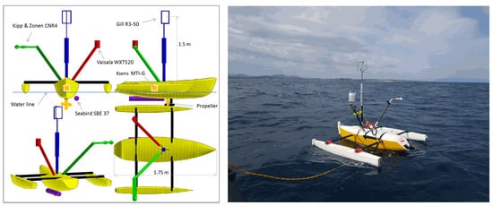
Figure 1.
Schema of the OCARINA platform [22] and deployment of it for the EURECA-OA project [45].
The observations were carried out at moderate winds (2–10 m/s) and averaged significant wave heights of 1.5 m. Most of the time, there was a swell, with an averaged wave age (the ratio between wave phase speed and wind speed) being equal to . Three flux calculation methods were used, namely, the EC, the ID, and the MOST (or bulk) methods. The best agreement of the estimates data was found by initially applying a mean bias to the values and by then using a constant imbalance term in the ID Method, which term was attributed to wave influence on the data. Overall, the confidence in the calculated estimated was found to be on the order of or 1–2 cm s−1, which is accurate, as shown in Figure 2.
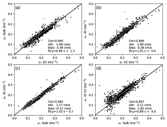
Figure 2.
Comparison of corrected EC, ID and bulk estimated of of B19. Please note that in panel (d), the ID S3 method is based on third-order structure functions of the wind (B19). (a) Corr:0.960, (b) Corr:0.966, (c) Corr:0.985, (d) Corr:0.897.
Most of the measurements were taken at a height that may be either considered to be in the midpart of the wave boundary layer (WBL) according to the rough estimation of 1–3 m given by [46] or well inside the WBL according to the definition of HS15, that is, at normalized heights , in wave-following coordinates (with k the wavenumber and the normal up to the water surface), ranging from 0.06 to 0.13, which is small compared to the their WBL height that peak at in their simulations, as reported in B19.
2.2. Wind-Wave Tunnel Experiment
2.2.1. Large Air-Sea Interaction Facility
The experiments in this study were carried out at the Large Air-Sea Interaction Facility (LASIF) of IRPHE and MIO Institutes in Marseille, France. This is a closed-circuit wind tunnel equipped with a 40 m long and 2.7 m wide water basin. For these experiments, the water depth was set to 0.9 m leading to an air channel height of 1.6 m (Figure 3).
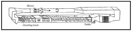
Figure 3.
Large wind-wave tunnel of the LASIF Facility in Luminy, Marseille (Copyright Hubert Branger).
The airflow is generated by an helicoidal wind fan (blower) and then it is directed to the upwind end of the tunnel through divergent and convergent sections. Before the entrance of the airflow at the water basin, a settling chamber equipped with a converging nozzle and a honeycomb-grid system is employed to laminarize the flow. The tunnel is slightly divergent to cancel the longitudinal pressure gradient due to wind generation, and to provide a constant flux surface boundary layer over the water surface. At the upwind end of the tunnel, a submerged piston wavemaker (e.g., mechanically actuated paddle) permits to simulate swell or longer waves, and two water pumps can be used to generate steady current conditions. It has to be noted that at the entrance of the water basin, a small metallic step generates additional turbulence on the airflow and thus a narrow transverse plastic bubble sheet was used to reduce the impact of the step on the airflow during the experiments.
At the downwind end of the test section, a permeable beach is mounted to reduce the wave reflection. At a 25 m fetch, a 5 m-long glass provides a clear view of the test section and allows to perform optical measurements that require a direct line of sight to the water surface. For a further description of the experimental facility, one can address to the previous works of [47,48].
2.2.2. Experimental Set-Up
Three parameters were measured: the wind speed in the middle of the air column, , which was solely used as a reference mean wind speed and ranged from 1 up to 14 m s−1; the wind velocity (or wind vector, depending on the wind sensor used) in the SBL at a variable height from 5 to 25 cm above the water surface; and the wave height. The instruments were arranged in the WWT as shown in Figure 4.
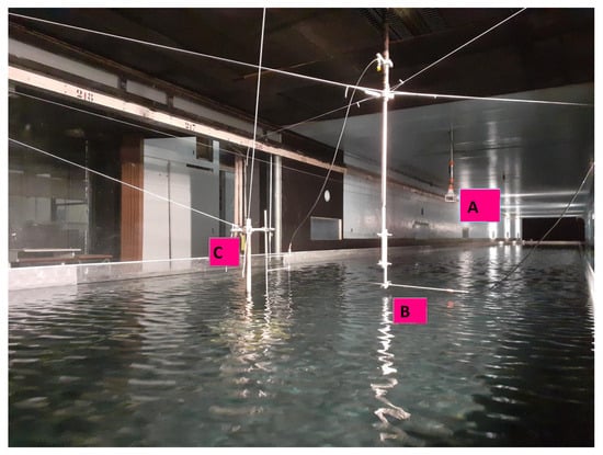
Figure 4.
Experimental configuration during the first Experiment: two-dimensional Windmaster Gill Co. sonic anemometer [A], Dantec hot film sensor [B], DISA capacitive wave gauge [C]. The fetch is at 26 m and the wind blows from the far right of the picture.
The experiments were conducted from April to July 2022, during which the main change was the use of different SBL wind-measuring probes, which are discussed above in this section. During this period, the water level had to be adjusted by adding small water quantities (∼1 cm) on a three to four-day basis in order to compensate evaporation phenomena. Lastly, repetitive calibrations of the wind and wave probes before, during, and after the experiments were necessary due to strong ambient temperature variations, as outlined below.
During the experiments, only two parameters were controlled: the rotation speed of the propeller (in rpm), which defined the mean wind speed in the WWT, , and the height of the SBL wind-measuring probe.
The mean reference velocity was measured using a Gill 2D sonic anemometer at an average height of 0.7 m above the water surface, which corresponds to 1.6 m above the water basin bottom. The sonic anemometer was also used to calibrate the other wind-measuring probes by placing each sensor next to it. The voltage output of each probe was compared to the measured velocity by the sonic anemometer, and a calibration law was extracted using a fourth-order polynomial interpolation over the entire range of tested wind velocities.
It should be noted that all the wave and wind sensors have analog outputs. Their signals were sampled at 256 Hz with a four-input 12-bits converter from National instruments. The analog signals entered an analog lowpass precision filter, which is intended to get rid of unavoidable disturbances around 50 Hz and harmonics, which are generated by power supplies, and which are transmitted by common mode voltages, in relation to minor issues with the grounding and the electromagnetic shielding of the fan motor controller. All are known issues at the facility and have no perceptible consequences on the presented results.
Wave measurements were made with a DISA capacitive probe, the accuracy of which was about one third of a millimeter after static calibration. As mentioned earlier, each time the water level was readjusted, one had to proceed to slight adjustments of the offset of the wave gauge.
Wind measurements were taken using CTA probes manufactured by Dantec Dynamics, Inc. (Skovlunde, Denmark) [49]. In order to increase our confidence in the performed wind measurements, we successively used probe types with enhanced capabilities: first a hot film probe, next a single wire probe, and at last a two-wire (or X-wire) probe.
The alignment of the CTA probes with the mean flow was carefully performed in the WWT with a technique that was probe-dependent, and which is not reported here for increasing the readability of the manuscript.
Probe calibrations were performed at constant steps of wind velocity for a ranging from 1 up to 14 m s−1. The total number of used steps ranged from ten to twenty according to the calibrated probe, since it was observed that some of the probes needed a refined calibration in medium winds.
The hot-film probe is robust, and we found it to be accurate to m s−1 at full range, and it is resistant to accidental immersion. As a counterpart, it has a slow time response, up to some Hz only. Therefore, it was only used to measure the mean wind profile in the SBL during the experiments.
Wire-type probes are highly fragile, a reason for which a clearance distance from the water was first set to 0.5, where was the dominant wave-length. This threshold was gradually decreased down to , when more confidence was gained in the peak height that the waves could reach.
For the calibration of of the X-wire probe, the voltage output was compared to the calibrated hot-film velocity data. Four-degree polynomials were also found to fit best the measurements of the reference sensor. It should be noted that during experiments, all the probes were successively mounted on the same vertical arm, the height of which was controlled with an accuracy on the order of 0.1 mm.
3. Results
3.1. Wind and Wave Characteristics
In the present section, the mean and turbulent SBL characteristics as well as wave characteristics are presented. They set the context for the later estimation of the friction velocity by several methods, and they already give some clues on the WBL characteristics.
3.1.1. Mean Airflow in the SBL
As a first test of our setup, five mean-wind profiles were calculated for (m s−1) = {3.15, 4.7, 8.12, 10.08, 13.85}. For each of those imposed values, the mean wind was successively estimated with the hot-film probe at ten heights that were empirically chosen, considering that more points would be required close to the surface where the log-profile curvature was expected to be larger, thus where a stretched height coverage was expected to be helpful.
The resulting profiles have an encouraging classical log-profile shape, specifically in light winds ( m s−1), and in the upper part of the SBL, as shown in Figure 5.
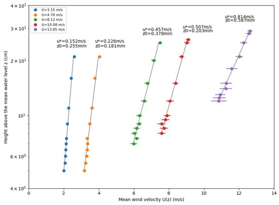
Figure 5.
Measured wind velocity U profiles for five wind conditions. The horizontal bar indicates the deviation of the measured wind. The grey lines are linear fit in semi-log coordinates.
In stronger winds ( m s−1), the lower parts of the profiles are fluctuating which is clearly visible in Figure 5. This behavior is attributed to the effect of waves on the SBL.
From these profiles, it was possible to get first estimated of and , which was straightforward by first linearly interpolating the data on semi-log coordinates, next by identifying the coefficients found in Equation (3), which is so-called the profile method. The and values in Figure 5 are slightly biased because they include outliers from the point of view of the SBL. Values that comply better with classical MOST were found by restricting the profiles to their central-part points, which better follows a logarithmic profile, as reported Table 1. The resulting and estimates globally increase with , as expected.

Table 1.
Estimates of and derived from the mean velocity profiles restricted to their logarithmic part. For reference, wind speed was extrapolated at 10 m by applying Equation (3) (, column 2).
3.1.2. Wave Characteristics
PSD functions of the time series of the water surface height were calculated for the wind-driven waves generated from the five above mentioned values, at which the airflow properties were investigated.
The generated waves have characteristics already well documented for the LASIF WWT at a 26 m fetch as reported in Table 2 and as shown in Figure 6. The variables reported in Table 2 are the peak period , the peak frequency , the significant wave height , the wavelength , and the phase speed , which were deduced from a linear dispersion relation. The so-called wave-age , where is the reference wind velocity at a 10 m height above the water surface, which was itself calculated with Equation (3), was also reported in Table 2, because it is helpful to distinguish swell () from wind-driven waves.
Table 2.
Characteristics of wind-driven waves.
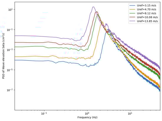
Figure 6.
Power spectra of wave elevation , for five different wind conditions.
3.1.3. Spectral Characteristics of Turbulence
In this section, the PSD functions and are reported as a function of and height. The results presented in this section were obtained with wire-probes, closer to the surface than in the previous section, i.e., at , as mentioned in Section 2.2.2, and with an arbitrarily selected different set of values, i.e., (m s−1) = {2, 2.3, 4, 6, 8, 10}. Therefore, the results presented hereafter may slightly differ from those of the above section. The new results were obtained in the second part of the experiments, when we had acquired more experience with the instruments’ calibration and SBL characteristics.
The spectra are clean and they all have a wide and well established log-log slope at frequencies in the range 10–30 Hz, over the full investigated wind velocity range, as shown in Figure 7 as sections of curves in orange color. These orange curves reveal the so-called inertial sub-range, where energy is transferred from larger to smaller wavelengths without production or dissipation. Note that the mean value of over the usable part of the inertial sub-range is the one used to apply the ID Method and to estimate , values of which are reported in the legend of Figure 7 (B19). Noticeably, waves have no clearly perceptible effect, even for the largest value, denoted by the upper brown curve in Figure 7.
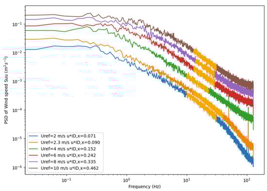
Figure 7.
Power spectra of the longitudinal wind velocity plotted as a function of frequency, for six different wind conditions at .
In contrast, the effect of the presence of waves significantly affects the co-spectra, which is visible as a well-defined peak at the same frequency of the observed most significant waves, as shown in Figure 8. Note that the data presented in Figure 7 and Figure 8 correspond to different experiments, namely constant-height SBL probe and varying reference wind velocity values in Figure 7, and varying SBL probe height and constant reference wind velocity in Figure 8. The counterparts of Figure 7 and Figure 8 are not shown for shortening the manuscript, but reveal similar features. Overall, it was found that the wave-induced peaks in the co-spectra, shown in Figure 8, were increasing with wind and decreasing with height, as may be expected.
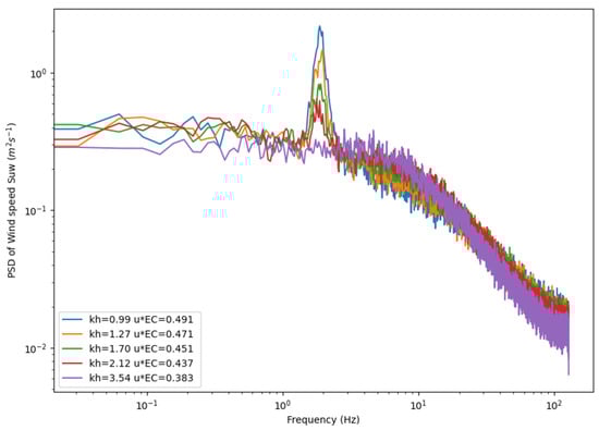
Figure 8.
Co-spectra at = 8 m s−1, for five different normalized heights kh (or ) above the water surface, where wind-driven waves at = 1.814 Hz are generated.
3.2. Wind Stress
3.2.1. Comparison Between and
For a constant measuring height and varying wind velocities, we find that the estimates of and have a good fit to each other, as reported in Table 3 and shown in Figure 9a. Although the correlation coefficient between and is excellent, i.e., close to unity, the rms value of is 0.045 m s−1, which is slightly less satisfying as it represents 20% of discrepancy with respect to the mean value of that is equal to 0.22 m s−1. Interestingly, the mean deviation between of − equals −0.075 m s−1, which is in agreement with the above-mentioned idea that (turbulent part of the stress) should be underestimated compared to (total stress). Note that the slope of the linear fit between and is equal to 0.76, which further indicates that the discrepancy between and is better defined as a ratio than as a bias.
Table 3.
and estimates for six different wind conditions.
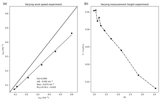
Figure 9.
Comparison of and for six wind speeds (a) and for ten measuring heights above the water surface (b). In (a), the term Corr stands for correlation coefficient between and , std is the standard deviation of , bias is the mean value of , and fit is the linear fit between the two variables.
In order to further analyze this ratio, extended measurements were performed at one speed velocity, = 8 m s−1, but for various heights, as reported in Table 4. The resulting ratio obtained is clearly departing from unity as the normalized height decreases, as shown in Figure 9b, which again may be interpreted as the fact that the turbulent part of the total stress decays as the wave influence increases.
Table 4.
Calculation of the imbalance term , and at = 8 m s−1.
3.2.2. Imbalance Term
Equation (8) may be rewritten as,
where and were intentionally neglected (Section 1.4). Therefore, the resulting estimates correspond to the purely turbulent part of the wind stress, which is a simple way to express that its calculation only results from the balance between production of turbulence by inertial effects and dissipation.
Now, if is considered to correspond to a wind stress that accounts for turbulence plus waves , one may rewrite Equation (9) to find as,
Subsequently, may be expressed as a function of and ,
At = 8 m s−1 and for wind-generated waves, the resulting values of were found to be in the range from 0.3 to 0.7, as reported in Table 4 and as shown in Figure 10.
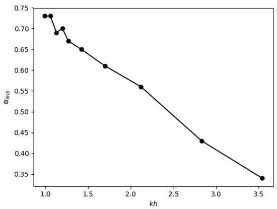
Figure 10.
Relation between and for ten measuring heights above the water surface, at = 8 m s−1.
Open sea data give comparable results, = 0.4, which is good (B19). However, measurements were performed at values in the range of 0.1–0.3 in B19, which is unfortunately out of scope of the values reachable in the WWT. Nevertheless, our results are encouraging as (1) the orders of magnitude of are almost equal in the lower range of WWT values, and (2) the WWT data show the decrease of the turbulent part of the stress close to the surface predicted by HS15, as reported Table 4, column 2.
Note that is not constant with height in Table 4 (column 3), which suggests that can not be assimilated to a total stress, which by definition would be constant with height, in agreement with HS15 claims. This is one limitation of our study, mostly for technical reasons, because HS15 used wave-following coordinates, whereas our measurements were made at fixed heights in the WWT. Subsequently, although it may hold, the hypothesis of a total flux that would be constant with height could not be confirmed by the present results. Overall, we consider the fact that we used Equation (12) to quantify as a preliminary approach.
4. Discussion
The present study allowed us to experimentally investigate some characteristics of the WBL present in the simulations of HS15. The collected data allow us to estimate the ratio between the turbulent stress and the turbulent plus wave-induced stress in the WBL as well as term.
Although our data suggest that increases as the distance from the water surface decreases, the variation of with height needs to be further investigated in order to perform a more thorough comparison between WWT and open sea data. Specifically, the pressure-correlation term and the turbulent transport of TKE need to be precisely measured in order to extract an accurate expression of them in a laboratory environment and to directly measure the remain part of total wind stress , i.e., the wave-induced wind stress.
Furthermore, although our result show that accounts for the turbulence plus waves, we could not confirm that it corresponded to a total flux, because was found to vary with height. This may partly be attributed to the fact that the HS15 hypothesis was emitted for wave-following measurements, whereas we extrapolated it to measurements made at constant height in the WWT. We plan to investigate this more thoroughly, by using wave-following probes in future experiments, on the basis of the methodology and hot-wire probe mounted on the linear actuator used by [50].
The discrepancies observed above between simulations, WWT data, and open-sea observations may be attributed to the challenging nature of the comparison performed here, as (1) simulations use idealized waves, (2) open-sea data may include multi-directional wave field and mixed swell and wind-driven wave conditions, and (3) WWT data were obtained in the presence of pure wind waves. Differences between WWT experiments and open sea conditions may also arise from differences in the vertical stratification of the SBL.
In short, the collected data are a first step before a more comprehensive data set is collected. However, it has to be noted that the present data should be further analyzed to better document the WBL height and other characteristics as a function of wind and wave properties. Other open questions that could be answered first regard the fact that the co-spectra of B19 do not fit the acknowledged co-spectra of [51]. In response, B19 suggested to fix this by defining a new normalized frequency that would depend on wave characteristics. The collected WWT data could help to elucidate this issue. Last, the simulations of HS15 show the presence of a low-level jet. We expect to check its existence in the future, with the help of the aforementioned wave-following probes.
5. Summary
In this study, our aim was to elucidate and the vertical profile of and of its components and . In order to maximize our confidence in the results, we decided to compare information from three sources, namely simulations, open sea data (B19), and WWT data. Another objective was to refine the definition of WBL, particularly its height as a function of wind velocity in WWT data.
The presented measurements were performed in the LASIF-WWT facility. Three wind-measuring probes were used to monitor the wind velocity in the SBL, namely a hot-film, a hot-wire, and an X-wire. Each probe was linked to a different friction velocity, , estimation method, namely the profile, the inertial-dissipation, and the eddy-correlation method. The use of the last two methods allowed us to advance in the reconciliation of and by defining the range of term and comparing it with the measured at open sea.
The collected data provided an unprecedented opportunity to estimate the ratio between the turbulent stress and the turbulent plus wave-induced stress in the WBL and to compare those estimates to the open sea data of B19. Our data suggest that increases as the distance from the water surface decreases. In addition, the order of height of is in the range of 0.3 to 0.7, which is comparable to the value of 0.4 found by B19.
Author Contributions
Conceptualization, conduct of the experiment and data analysis, L.V. and D.B.; Experiment and setup, C.L.; Further data analysis, S.B.; writing—review and editing plus science advices, J.T., A.S., A.V. and P.F. All authors have read and agreed to the published version of the manuscript.
Funding
This research received no external funding.
Institutional Review Board Statement
Not applicable.
Informed Consent Statement
Not applicable.
Data Availability Statement
The raw and meta data are available upon request from denis.bourras@mio.osupytheas.fr.
Acknowledgments
The authors are grateful to Hubert Branger for his continuous and invaluable help, and for fruitful discussions on wind-wave tank experiments and on the challenging art of making accurate measurements. The authors would also like to thank Ecole Centrale de Nantes, France, the MIO-OPLC physics team for making possible and funding the training period of L. Vonta, and OSU Institut-Pythéas UAR 3470 CNRS for letting our team conduct the experiment at the large Air-Sea wind-wave facility of Luminy, Marseille.
Conflicts of Interest
The authors declare no conflicts of interest.
References
- Miles, J.W. On the generation of surface waves by shear flows. J. Fluid Mech. 1957, 3, 185. [Google Scholar] [CrossRef]
- Donelan, M.A.; Haus, B.K.; Reul, N.; Plant, W.J.; Stiassnie, M.; Graber, H.C.; Brown, O.B.; Saltzman, E.S. On the limiting aerodynamic roughness of the ocean in very strong winds. Geophys. Res. Lett. 2004, 31, 2004GL019460. [Google Scholar] [CrossRef]
- Monin, A.; Obukhov, A. Basic Laws of Turbulent Mixing in the Surface Layer of the Atmosphere. Contrib. Geophys. Inst. Acad. Sci. USSR 1954, 24, 163–187. [Google Scholar]
- Obukhov, A.M. Turbulence in an atmosphere with a non-uniform temperature. Bound.-Layer Meteorol. 1971, 2, 7–29. [Google Scholar] [CrossRef]
- Businger, J.A.; Wyngaard, J.C.; Izumi, Y.; Bradley, E.F. Flux-Profile Relationships in the Atmospheric Surface Layer. J. Atmos. Sci. 1971, 28, 181–189. [Google Scholar] [CrossRef]
- Champagne, F.H.; Friehe, C.A.; LaRue, J.C.; Wynagaard, J.C. Flux Measurements, Flux Estimation Techniques, and Fine-Scale Turbulence Measurements in the Unstable Surface Layer Over Land. J. Atmos. Sci. 1977, 34, 515–530. [Google Scholar] [CrossRef]
- Kaimal, J.C.; Wyngaard, J.C. The Kansas and Minnesota experiments. Bound.-Layer Meteorol. 1990, 50, 31–47. [Google Scholar] [CrossRef]
- Fairall, C.W.; Banner, M.L.; Peirson, W.L.; Asher, W.; Morison, R.P. Investigation of the physical scaling of sea spray spume droplet production. J. Geophys. Res. Oceans 2009, 114, 2008JC004918. [Google Scholar] [CrossRef]
- Bruch, W. Experimental and Numerical Study of Sea Spray Generation and Transport, and Their Consequences on the Properties of the Marine Atmospheric Boundary Layer. Ph.D. Thesis, University of Toulon, La Garde, France, 2021. [Google Scholar]
- Kudryavtsev, V.N.; Makin, V.K. Impact of Ocean Spray on the Dynamics of the Marine Atmospheric Boundary Layer. Bound.-Layer Meteorol. 2011, 140, 383–410. [Google Scholar] [CrossRef]
- Geernaert, G.L.; Katsaros, K.B.; Richter, K. Variation of the drag coefficient and its dependence on sea state. J. Geophys. Res. Oceans 1986, 91, 7667–7679. [Google Scholar] [CrossRef]
- Donelan, M.A.; Dobson, F.W.; Smith, S.D.; Anderson, R.J. On the Dependence of Sea Surface Roughness on Wave Development. J. Phys. Oceanogr. 1993, 23, 2143–2149. [Google Scholar] [CrossRef]
- Hsu, C.T.; Hsu, E.Y.; Street, R.L. On the structure of turbulent flow over a progressive water wave: Theory and experiment in a transformed, wave-following co-ordinate system. J. Fluid Mech. 1981, 105, 87. [Google Scholar] [CrossRef]
- Belcher, S.E.; Hunt, J.C.R. Turbulent shear flow over slowly moving waves. J. Fluid Mech. 1993, 251, 109–148. [Google Scholar] [CrossRef]
- Edson, J.B.; Fairall, C.W. Similarity Relationships in the Marine Atmospheric Surface Layer for Terms in the TKE and Scalar Variance Budgets. J. Atmospheric Sci. 1998, 55, 2311–2328. [Google Scholar] [CrossRef]
- Smith, S.D. Coefficients for sea surface wind stress, heat flux, and wind profiles as a function of wind speed and temperature. J. Geophys. Res. Oceans 1988, 93, 15467–15472. [Google Scholar] [CrossRef]
- Charnock, H. Wind stress on a water surface. Q. J. R. Meteorol. Soc. 1955, 81, 639–640. [Google Scholar] [CrossRef]
- Edson, J.B.; Jampana, V.; Weller, R.A.; Bigorre, S.P.; Plueddemann, A.J.; Fairall, C.W.; Miller, S.D.; Mahrt, L.; Vickers, D.; Hersbach, H. On the Exchange of Momentum over the Open Ocean. J. Phys. Oceanogr. 2013, 43, 1589–1610. [Google Scholar] [CrossRef]
- Edson, J.; Crawford, T.; Crescenti, J.; Farrar, T.; Frew, N.; Gerbi, G.; Helmis, C.; Hristov, T.; Khelif, D.; Jessup, A.; et al. The Coupled Boundary Layers and Air–Sea Transfer Experiment in Low Winds. Bull. Am. Meteorol. Soc. 2007, 88, 341–356. [Google Scholar] [CrossRef]
- Soloviev, Y.P.; Kudryavtsev, V.N. Wind-Speed Undulations Over Swell: Field Experiment and Interpretation. Bound.-Layer Meteorol. 2010, 136, 341–363. [Google Scholar] [CrossRef]
- Katsaros, K.B. The aqueous thermal boundary layer. Bound.-Layer Meteorol. 1980, 18, 107–127. [Google Scholar] [CrossRef]
- Bourras, D.; Branger, H.; Reverdin, G.; Marié, L.; Cambra, R.; Baggio, L.; Caudoux, C.; Caudal, G.; Morisset, S.; Geyskens, N.; et al. A New Platform for the Determination of Air–Sea Fluxes (OCARINA): Overview and First Results. J. Atmospheric Ocean. Technol. 2014, 31, 1043–1062. [Google Scholar] [CrossRef]
- Fujitani, T. Direct measurement of turbulent fluxes over the sea during AMTEX. Pap. Meteorol. Geophys. 1981, 32, 119–134. [Google Scholar] [CrossRef]
- Fujitani, T. Method of turbulent flux measurement on a ship by using a stable platform system. Pap. Meteorol. Geophys. 1985, 36, 157–170. [Google Scholar] [CrossRef]
- Tsukamoto, O.; Ohtaki, E.; Ishida, H.; Horiguchi, M.; Mitsuta, Y. On-Board Direct Measurements of Turbulent Fluxes over the Open Sea. J. Meteorol. Soc. Jpn. Ser. II 1990, 68, 203–211. [Google Scholar]
- Bradley, E.F.; Coppin, P.A.; Godfrey, J.S. Measurements of sensible and latent heat flux in the western equatorial Pacific Ocean. J. Geophys. Res. Oceans 1991, 96, 3375–3389. [Google Scholar] [CrossRef]
- Fairall, C.W.; White, A.B.; Edson, J.B.; Hare, J.E. Integrated Shipboard Measurements of the Marine Boundary Layer. J. Atmospheric Ocean. Technol. 1997, 14, 338–359. [Google Scholar] [CrossRef]
- Edson, J.B.; Hinton, A.A.; Prada, K.E.; Hare, J.E.; Fairall, C.W. Direct Covariance Flux Estimates from Mobile Platforms at Sea. J. Atmospheric Ocean. Technol. 1998, 15, 547–562. [Google Scholar] [CrossRef]
- Webster, P.J.; Lukas, R. TOGA COARE: The Coupled Ocean—Atmosphere Response Experiment. Bull. Am. Meteorol. Soc. 1992, 73, 1377–1416. [Google Scholar] [CrossRef]
- Kawamura, H.; Okuda, K.; Kawai, S.; Toba, Y. Structure of Turbulent Boundary Layer over Wind Waves in a Wind Wave Tunnel. Ph.D. Thesis, Tohoku University, Tokyo, Japan, 1981. Volume 28. pp. 69–86. [Google Scholar]
- Lai, R.J.; Shemdin, O.H. Laboratory investigation of air turbulence above simple water waves. J. Geophys. Res. Oceans 1971, 76, 7334–7350. [Google Scholar] [CrossRef]
- Buckley, M.; Veron, F. The turbulent airflow over wind generated surface waves. Eur. J. Mech.-B/Fluids 2019, 73, 132–143. [Google Scholar] [CrossRef]
- Bourras, D.; Cambra, R.; Marié, L.; Bouin, M.; Baggio, L.; Branger, H.; Beghoura, H.; Reverdin, G.; Dewitte, B.; Paulmier, A.; et al. Air-Sea Turbulent Fluxes From a Wave-Following Platform During Six Experiments at Sea. J. Geophys. Res. Oceans 2019, 124, 4290–4321. [Google Scholar] [CrossRef]
- Donelan, M.A.; Drennan, W.M.; Katsaros, K.B. The Air–Sea Momentum Flux in Conditions of Wind Sea and Swell. J. Phys. Oceanogr. 1997, 27, 2087–2099. [Google Scholar] [CrossRef]
- Bruch, W.; Conan, B. Mean Wind Profile Departure from Log-Law in the Lower Marine Atmospheric Boundary Layer for Different Wave-Wind Conditions Using Scanning Wind LiDAR Measurements. Available online: https://hal.science/hal-04984296v1 (accessed on 23 March 2025).
- Elfouhaily, T.; Vandemark, D.; Gourrion, J.; Chapron, B. Estimation of wind stress using dual-frequency TOPEX data. J. Geophys. Res. Oceans 1998, 103, 25101–25108. [Google Scholar] [CrossRef]
- Hara, T.; Sullivan, P.P. Wave Boundary Layer Turbulence over Surface Waves in a Strongly Forced Condition. J. Phys. Oceanogr. 2015, 45, 868–883. [Google Scholar] [CrossRef]
- Pedreros, R.; Dardier, G.; Dupuis, H.; Graber, H.C.; Drennan, W.M.; Weill, A.; Guérin, C.; Nacass, P. Momentum and heat fluxes via the eddy correlation method on the R/V L’Atalante and an ASIS buoy. J. Geophys. Res. Oceans 2003, 108, 2002JC001449. [Google Scholar] [CrossRef]
- Kolmogorov, A.N. Air–Sea Interaction in the Southern Ocean: Exploring the Height of the Wave Boundary Layer at the Air–Sea Interface. Doklady Akademii Nauk SSSR 1941, 30, 301–304. [Google Scholar]
- Dupuis, H.; Taylor, P.K.; Weill, A.; Katsaros, K. Inertial dissipation method applied to derive turbulent fluxes over the ocean during the Surface of the Ocean, Fluxes and Interactions with the Atmosphere/Atlantic Stratocumulus Transition Experiment (SOFIA/ASTEX) and Structure des Echanges Mer-Atmosphere, Proprietes des Heterogeneites Oceaniques: Recherche Experimentale (SEMAPHORE) experiments with low to moderate wind speeds. J. Geophys. Res. Oceans 1997, 102, 21115–21129. [Google Scholar] [CrossRef]
- Taylor, P.K.; Yelland, M.J. The Dependence of Sea Surface Roughness on the Height and Steepness of the Waves. J. Phys. Oceanogr. 2001, 31, 572–590. [Google Scholar] [CrossRef]
- Bourras, D.; Weill, A.; Caniaux, G.; Eymard, L.; Bourlès, B.; Letourneur, S.; Legain, D.; Key, E.; Baudin, F.; Piguet, B.; et al. Turbulent air-sea fluxes in the Gulf of Guinea during the AMMA experiment. J. Geophys. Res. Oceans 2009, 114, 2008JC004951. [Google Scholar] [CrossRef]
- Stull, R.B. An Introduction to Boundary Layer Meteorology; Springer Science & Business Media: Berlin/Heidelberg, Germany, 1988. [Google Scholar] [CrossRef]
- Bourras, D.; Cambra, R.; Marie, L.; Bouin, M.N.; Baggio, L.; Branger, H.; Beghoura, H.; Reverdin, G.; Dewitte, B.; Paulmier, A.; et al. OCARINA (Ocean coupled to the atmosphere: Instrumented research on an auxiliary ship). J. Geophys. Res. Oceans 2019. [Google Scholar] [CrossRef]
- Bourras, D.; Branger, H.; Luneau, C.; Reverdin, G.; Speich, S.; Geykens, N.; Barrois, H.; Clémençon, A. EUREC4A-OA_OCARINA: OCARINA Air-Sea Flux Data. Available online: https://hal.science/hal-03066519/document (accessed on 8 December 2020).
- Cifuentes-Lorenzen, A.; Edson, J.B.; Zappa, C.J. Air–Sea Interaction in the Southern Ocean: Exploring the Height of the Wave Boundary Layer at the Air–Sea Interface. Bound.-Layer Meteorol. 2018, 169, 461–482. [Google Scholar] [CrossRef]
- Villefer, A.; Benoit, M.; Violeau, D.; Luneau, C.; Branger, H. Influence of Following, Regular, and Irregular Long Waves on Wind-Wave Growth with Fetch: An Experimental Study. J. Phys. Oceanogr. 2021, 51, 3435–3448. [Google Scholar] [CrossRef]
- Coantic, M.; Ramamonjiarisoa, A.; Mestayer, P.; Resch, F.; Favre, A. Wind-water tunnel simulation of small-scale ocean-atmosphere interactions. J. Geophys. Res. Oceans 1981, 86, 6607–6626. [Google Scholar] [CrossRef]
- Jørgsen, F.E. How to Measure Turbulence with Hot-Wire Anemometers—A Practical Guide. Available online: https://web.iitd.ac.in/~pmvs/courses/mel705/hotwire2.pdf (accessed on 8 December 2020).
- Grare, L.; Peirson, W.L.; Branger, H.; Walker, J.W.; Giovanangeli, J.P.; Makin, V. Growth and dissipation of wind-forced, deep-water waves. J. Fluid Mech. 2013, 722, 5–50. [Google Scholar] [CrossRef]
- Kaimal, J.C.; Wyngaard, J.C.; Izumi, Y.; Coté, O.R. Spectral characteristics of surface-layer turbulence. Q. J. R. Meteorol. Soc. 1972, 98, 563–589. [Google Scholar] [CrossRef]
Disclaimer/Publisher’s Note: The statements, opinions and data contained in all publications are solely those of the individual author(s) and contributor(s) and not of MDPI and/or the editor(s). MDPI and/or the editor(s) disclaim responsibility for any injury to people or property resulting from any ideas, methods, instructions or products referred to in the content. |
© 2025 by the authors. Licensee MDPI, Basel, Switzerland. This article is an open access article distributed under the terms and conditions of the Creative Commons Attribution (CC BY) license (https://creativecommons.org/licenses/by/4.0/).