Impact of Large Eddies on Flux-Gradient Relations in the Unstable Surface Layer Based on Measurements over the Tibetan Plateau

Abstract

The Monin-Obukhov similarity theory (MOST) is widely used for surface layer parameterization. Discrepancies in MOST highlight the need to account for large eddy effects. A possible solution is to introduce the boundary layer depth $z_i$ as a new scaling parameter, which may enhance the applicability of the theory. A novel similarity scheme has recently been proposed to explicitly account for large eddy effects under unstable conditions. In this study, we estimated the impact of large eddies on the unstable surface layer using field measurements from a summer experiment on the Tibetan Plateau. Furthermore, we evaluated the proposed scheme and suggested simplifications for its improvements. In this study, the non-dimensional wind shear, ${\varphi }_m$, exhibited greater scatter and larger deviations from MOST than the non-dimensional temperature gradient, ${\varphi }_h$. Additionally, the normalized wind gradient ${\varphi }_m$ is found to depend on both $z/L$ and $z_i/L$, where $z$ is height above ground and $L$ is the Monin-Obukhov length. The additional dependence on $z_i/L$ suggests that it may serve as a crucial missing scaling parameter in the MOST under unstable conditions. Ultimately, we observed that the $z_i$-scaling parameter $C_m$ derived from the proposed scheme maintains a linear correlation with the stability parameter ($-z_i/L$), confirming the scheme’s effectiveness. Moreover, vertical wind gradients, friction velocity, and momentum flux predicted by this new scheme align more closely with observations than those estimated using the classical similarity function, thereby strengthening its feasibility and offers valuable insights for its simplification for Earth System modeling.

1. Introduction

Surface-atmosphere exchanges (i.e., surface fluxes) of energy, mass and momentum are essential for quantifying various processes involved in the land-atmosphere interactions. Their parameterization is thus of fundamental importance in numerical meteorology and climate models. Since its proposal, the Monin-Obukhov similarity theory (MOST) [1] has been a widely accepted pragmatic framework for the surface flux parameterization.

The conventional MOST theory relies on the assumption of horizontal homogeneity and statistical stationarity. It applies dimensionless functions to characterize the impact of atmospheric stability, represented by $z/L$, on turbulence-related quantities, such as wind speed and temperature. In this framework, $z$ corresponds to the height above the surface, and $L$ represents the Obukhov length. Since its proposal, MOST has undergone thorough validation in field experiments examining wind and temperature gradients in the atmospheric surface layer, with various empirical functions derived to quantify these relationships [2,3,4,5,6]. These empirical functions are commonly applied in atmospheric models to estimate surface fluxes. However, numerous studies have documented significant deviations in their performance, highlighting discrepancies across different atmospheric stability regimes [7,8,9,10,11]. Such discrepancies are generally caused by neglected physical processes in MOST and unavoidable random fluctuations [12]. As emphasized in foundational works such as [13], refinements to similarity theory often require additional dimensionless parameters and scaling considerations beyond those typically invoked in MOST.

Over the past decade, many studies have highlighted the impact of large-scale eddies on the surface layer and their relevance to MOST [11,14,15,16,17,18,19,20,21,22,23]. As proposed by [13], these large eddies can be effectively represented by integrating boundary-layer depth ($z_i$) into universal similarity functions. Through turbulence-resolving large-eddy simulations (LES), it was highlighted in [8] that accounting for large-scale eddies ($z_i$-scale) is important in the parameterization of both mean gradients and normalized variance. This conclusion was supported by field measurements from [24].However, the exact formulation of the similarity function that considers the influence of large eddies remains undefined based on these data.

A recent study by [25], using Large Eddy Simulations (LES), examined the influence of large eddies on surface-layer properties. The study quantitatively assessed the effect of large convective eddy processes under convective conditions through a three-dimensional multiscale analysis. Their findings demonstrated that the dimensionless wind gradient is influenced by both $z$ and $z_i$, suggesting that ${\varphi }_m={\varphi }_m(z/L,z/z_i)$, with the normalized temperature gradient satisfying the MOST hypothesis. Based on their LES data, they proposed a revised similarity function for the unstable surface layer.

In this work, we offer evidence supporting the relevance of boundary layer height in the surface layer. Moreover, we evaluate the applicability of the revised similarity function by [25] to the unstable surface layer. Data for this study were obtained from two summer field campaigns conducted on the Tibetan Plateau (TP), encompassing standard surface layer measurements (such as profiles and turbulent fluxes) as well as comprehensive information on boundary layer height. The paper is organized as follows. Section 2 presents the theoretical background of MOST, the proposed universal function, and a brief overview of the TIPEX-III dataset. The results of the field data analysis are presented in Section 3, followed by the discussion and conclusion in Section 4.

2. Theory and Experimental Data

2.1. Monin-Obukhov Similarity Theory and Classical Flux-Gradient Relations

With the assumption of surface homogeneity and a steady-state flow, MOST states that the statistical quantities in the surface layer are are normalized using four independent parameters: measurement height $z$, friction velocity $u_{*}$, near-surface kinematic heat flux $\overline{{(w^{\prime }{\theta }^{\prime })}_0}$, and the buoyancy parameter $g/{\Theta }_0$. It should be noted that $w^{\prime }$ and ${\theta }^{\prime }$ are the deviations from the mean wind and temperature, respectively, whereas ${\Theta }_0$ denotes the mean potential temperature within the surface layer. The resulting normalized parameters yield a single dimensionless stability parameter $\zeta =z/L$, where

$$L=-{\displaystyle \frac{u_{*}^3{\Theta }_0}{\kappa g\overline{{(w^{\prime }{\theta }^{\prime })}_0}}}$$

(1)

is the Obukhov length. Here, $\kappa$ refers to the von Kármán constant, $g$ is the gravitational acceleration, and ${\theta }_{*}$ represents the dimensionless temperature scale. The subscript 0 denotes the value at the surface.

Following the principles of MOST, any mean flow or turbulence-related quantity in the surface layer is described by a universal function dependent on $z/L$. Hence, the non-dimensional gradients of wind and temperature can be expressed as

$${\displaystyle \frac{\kappa z}{u_{*}}}{\displaystyle \frac{\partial U}{\partial z}}={\varphi }_m({\displaystyle \frac{z}{L}})$$

(2)

$${\displaystyle \frac{\kappa z}{{\theta }_{*}}}{\displaystyle \frac{\partial \Theta }{\partial z}}={\varphi }_h({\displaystyle \frac{z}{L}})$$

(3)

where $U$ and $\Theta$ represent the mean wind speed and temperature. ${\varphi }_m({\displaystyle \frac{z}{L}})$ and ${\varphi }_h({\displaystyle \frac{z}{L}})$ are the universal similarity functions.

By deriving $u_{*}$ and ${\theta }_{*}$ in Equations (2) and (3), we can calculate the surface fluxes of momentum ($\mathsf{\tau }$) and sensible heat ($\mathrm{H}$), as defined below:

$$\mathsf{\tau }=\rho u_{*}^2$$

(4)

$$\mathrm{H}=-\rho c_p{u}_{*}{\theta }_{*},$$

(5)

where $\rho$ is air density and $c_p$ is specific heat capacity under constant pressure.

Following the establishment of the Monin–Obukhov Similarity Theory (MOST), numerous field experiments have been conducted to determine the universal similarity functions for momentum and sensible heat transfer, denoted as ${\varphi }_m({\displaystyle \frac{z}{L}})$ and ${\varphi }_h({\displaystyle \frac{z}{L}})$. Early influential studies by [2,3,5] provided empirical formulations for the unstable surface layer. These formulations are given by

$${\varphi }_m({\displaystyle \frac{z}{L}})={(1-{\gamma }_m{\displaystyle \frac{z}{L}})}^{-1/4}$$

(6)

$${\varphi }_h({\displaystyle \frac{z}{L}})=\beta {(1-{\gamma }_h{\displaystyle \frac{z}{L}})}^{-1/2}$$

(7)

Notably, the empirical constants vary among studies: The parameters ${\gamma }_m=15$,${\gamma }_h=9$, and $\beta =0.74$ were proposed in [2]; ${\gamma }_m={\gamma }_h=16$ with $\beta =1$ were used in Ref. [3]; and ${\gamma }_m=15.2$, ${\gamma }_h=11.6$, and $\beta =0.95$ were reported in Ref. [5]. Additionally, according to an overview cited as Ref. [6], an alternative set of parameters for the unstable surface layer is presented as

$${\varphi }_m({\displaystyle \frac{z}{L}})={(1-19{\displaystyle \frac{z}{L}})}^{-1/4}$$

(8)

$${\varphi }_h({\displaystyle \frac{z}{L}})=0.95{(1-11.6{\displaystyle \frac{z}{L}})}^{-1/2}$$

(9)

2.2. Improved Flux-Gradient Relations Accounting for Large Eddy Effects

To account for large-eddy influences, a revised universal similarity function was introduced in [25] that explicitly incorporates boundary layer depth ($z_i$) into the traditional MOST framework. Under convective conditions, this boundary layer depth ($z_i$) can range from a few hundred meters to over two kilometers, reflecting large-eddy structures that conventional surface-layer scaling alone may not capture. The form of the universal function is:

$${\varphi }_m=C_m{(-{\displaystyle \frac{z}{L}})}^{-1/3}{(1-\alpha {\displaystyle \frac{z}{z_i}})}^{2/3}$$

(10)

Here, $\alpha$ is defined as the ratio of $z_i$ (the boundary layer height) to the height at which the heat flux becomes zero, $z_0$. Mathematically, $\alpha ={\displaystyle \frac{z_i}{z_0}}$. $C_m$ is a function of $-z_i/L$ and linearly related to it:

$$C_m=f_{linear}(-{\displaystyle \frac{z_i}{L}})$$

(11)

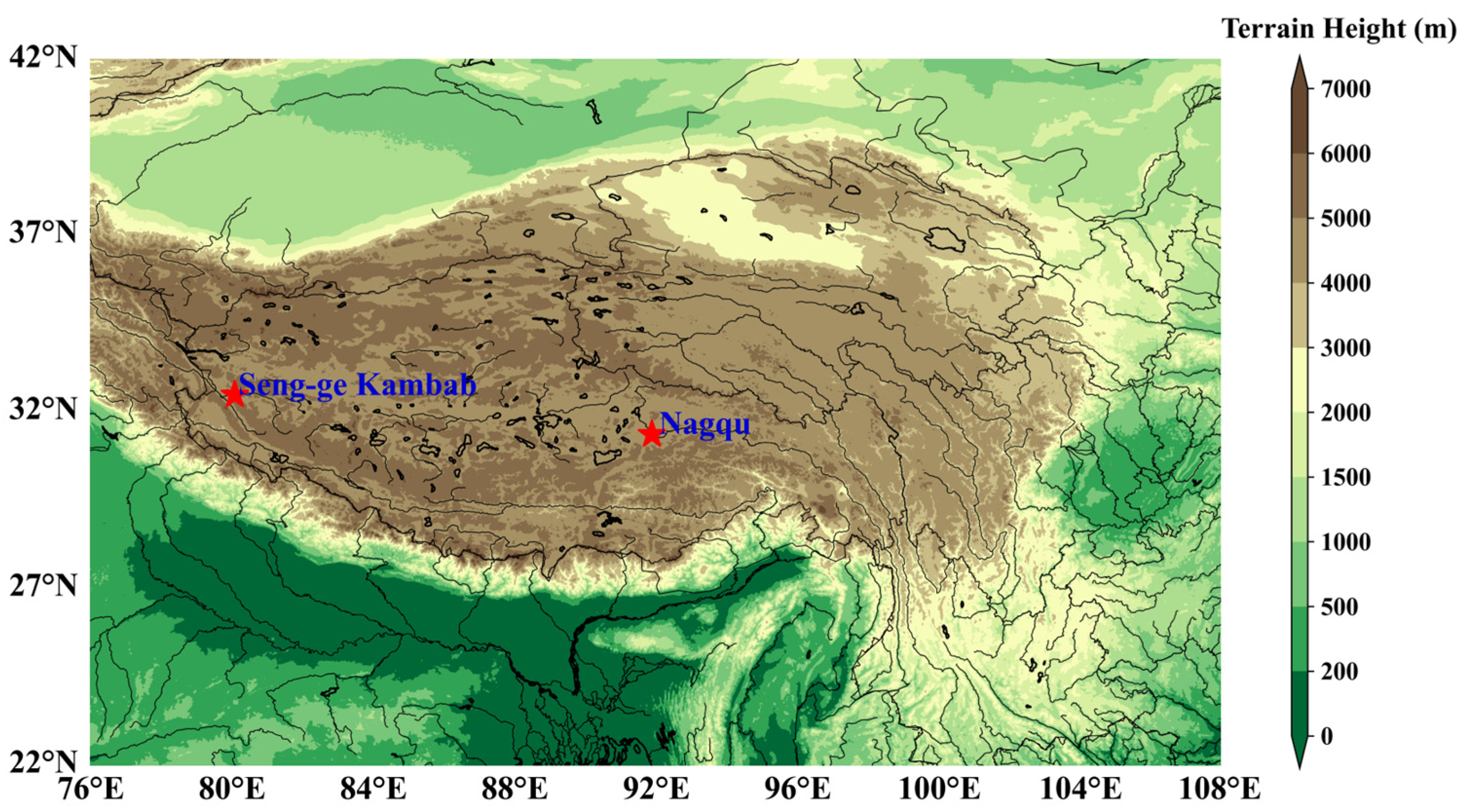
2.3. TIPEX-III Dataset and Data Processing

The ASL data used in this study were obtained from the Third Tibetan Atmospheric Scientific Experiment (TIPEX-III) [26], covering the summer seasons of 2014 and 2015. Two observational sites were selected for this study: one located at Seng-ge Kambab in the western TP and the other at Nagqu in the central TP, as shown in Figure 1.

Table 1. Geographical Features and Data Sampling Characteristics at the Two Sites Used in This Study.

Site Location	Longitude and Latitude	Elevation (m)	Land Cover Type	Observation Heights (m)	Sonic Anemometer Height (m)
Seng-ge Kambab	80.1° E, 32.5° N	4278	Bare soil with few obstacles	1, 2, 4, 8, 18	5
Nagqu	91.9° E, 31.4° N	4509	Alpine steppe	0.75, 1.5, 3, 6, 12	3.02

Five 010 wind speed sensor (with an accuracy of 0.07 m s⁻¹; made by Met One) and five HMP155A air temperature T (with an accuracy of 0.226 °C − 0.0028 °C × T when −80°C < T < 20 °C and 0.055 °C + 0.0057 °C × T when 20°C < T < 60 °C, made by Campbell Scientific, Logan, UT, USA)) are used for Seng-ge Kambab and Nagqu sites. Both Seng-ge Kambab and Nagqu sites are equipped with only one tower, which is used to measure wind speed and vertical gradients at multiple heights. At the Seng-ge Kambab site, a 3d sonic anemometer (CSAT3A, Campbell Scientific Inc., Logan, UT, USA) and a gas analyzer (EC150, Campbell Scientific Inc., Logan, UT, USA) are used, whereas the Nagqu site employs a 3d sonic anemometer (CSAT3, Campbell Scientific Inc., Logan, UT, USA) and a CO₂/H₂O open-path gas analyzer (LI-7500, LI-COR , Lincoln, NE, USA).

provides the geographical and tower sensor information for both flux observation sites. Both towers were positioned in a relatively flat region within the lowest 20 m of the atmosphere, making it an ideal site for testing the similarity theory. The raw data collected at a frequency of 10 Hz from sonic anemometers at the flux measurement sites were utilized to calculate turbulence fluxes and the Obukhov length. The turbulent fluxes were computed using the eddy covariance method across multiple sites. Detailed information on the quality control procedures is available in [27]. Vertical profiles of mean wind and temperature, as well as wind data, were retrieved from the sensors every 30 min.

The planetary boundary layer height (PBLH) data for Seng-ge Kambab and Nagqu during the summers of 2014 and 2015 were obtained from [28]. Building on the potential temperature gradient method proposed by [29], routine meteorological intensive-sounding data from Seng-ge Kambab and Nagqu were used to estimate the PBLH. This approach hinges on identifying sharp variations in the vertical distribution of potential temperature, thereby delineating the transition from the turbulent boundary layer to the more stable free atmosphere. In their study, the PBL is categorized into three types: convective boundary layer (CBL), neutral boundary layer (NBL), and stable boundary layer (SBL). PBLH observations were conducted at 08:00 BJT (00:00 UTC), 14:00 BJT (06:00 UTC), and 20:00 BJT (12:00 UTC) each day.

The dataset was limited because PBLH observations, profile measurements, and turbulence data were not available for all days. Following quality control of the observational sounding data, the selected periods for analysis included 19 July to 31 August 2014 and 1 June to 31 August 2015 at Seng-ge Kambab, and 1 June to 31 August 2015 at Nagqu. The criteria for data acceptance, beyond completeness, were as follows: (i) vertical wind gradient greater than 0 ${\mathrm{s}}^{-1}$ and vertical temperature gradient less than 0 $\mathrm{K}{\mathrm{m}}^{-1}$; (ii) sensible heat flux (SHF) greater than 20 $\mathrm{W}{\mathrm{m}}^{-2}$; (iii) friction velocity ($u_{*}$) greater than 0.05 $\mathrm{m}{\mathrm{s}}^{-1}$; and (iv) Obukhov length ($L$) greater than −200 m and less than −1 m. It should be noted that the original TIPEX-III dataset for the Nagqu station encompassed measurements at 0.75, 1.5, 3, 6, 12, and 22 m. However, due to temperature inversions and pronounced wind speed variations observed at the 22-m level, only data from 0.75, 1.5, 3, 6, and 12 m were analyzed in this study (see Table 1). Based on these available measurements, we selected an intermediate height to represent the gradient level. For example, the gradient levels of Nagqu station are 1.125, 2.25, 4.5, and 9 m.

3. Results

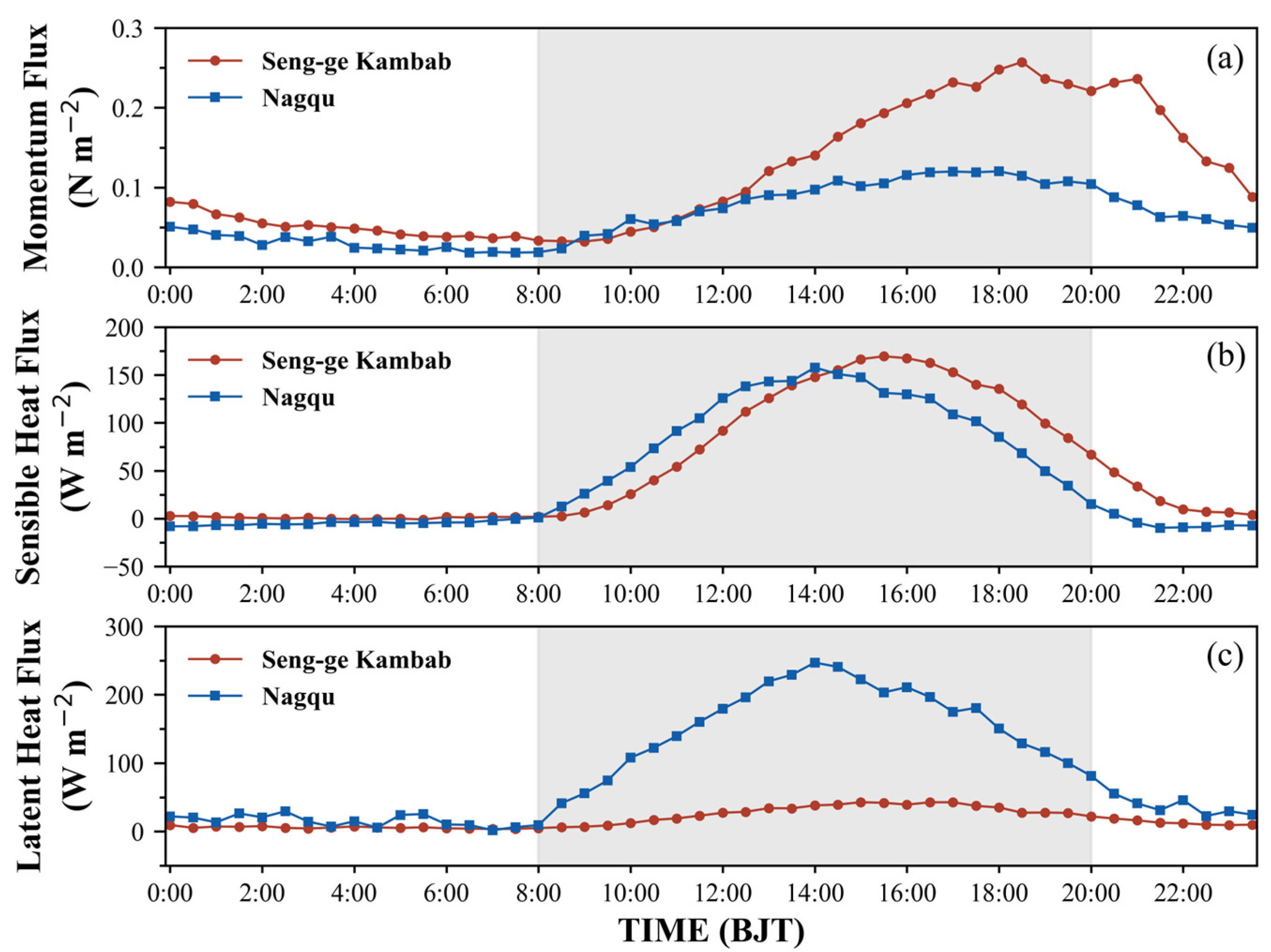
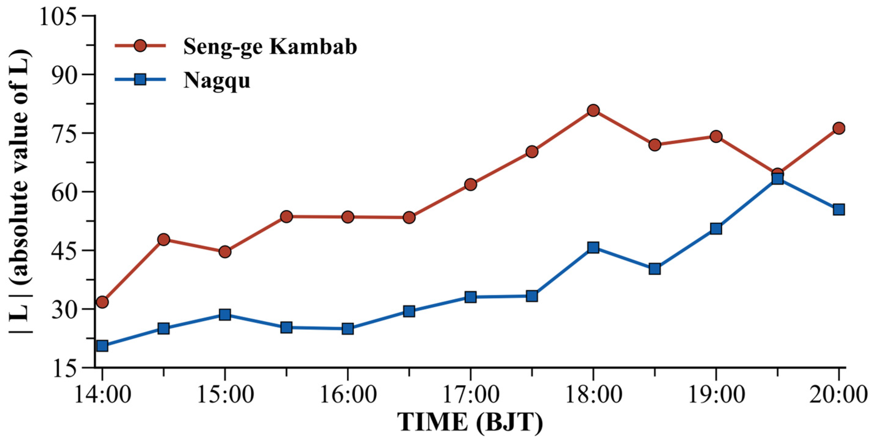
3.1. Turbulence Characteristics in the Unstable Surface Layer over the Tibetan Plateau

Figure 2 shows the diurnal variation of momentum flux ($\tau$), sensible heat flux (SHF), and latent heat flux (LHF), averaged over the study period at Seng-ge Kambab and Nagqu. The period from 08:00 to 20:00 is shaded in gray to denote daylight hours on the Tibetan Plateau. A clear diurnal pattern is observed in both momentum flux and heat flux, with lower values during the night and an increase after sunrise, primarily due to increased solar radiation and the enhancement of atmospheric mixing. However, the diurnal variation of latent heat flux at the Seng-ge Kambab site is less evident (Figure 2c), which may be influenced by regional factors, including variations in surface moisture or cloud cover, that affect latent heat exchange differently. Figure 2a,b show that the maximum SHF occurs around 15:00 BJT at both sites, while momentum flux reaches its peak at 18:00 BJT. This time lag suggests that the momentum flux generally responds more slowly to solar heating and atmospheric turbulence than the sensible heat flux. This can be explained based on the budget equations of momentum flux and heat flux. The sensible heat flux is primarily driven by surface heating and buoyancy-induced turbulence, leading to a rapid response to solar heating. In contrast, the momentum flux is influenced by wind shear and turbulent mixing, which have longer adjustment timescales due to inertial effects and the dependence on large-scale pressure gradients. Consequently, the momentum flux lags behind the sensible heat flux in response to diurnal variations in solar radiation.

The Monin-Obukhov similarity theory was developed to describe the statistical structure of the atmospheric surface layer, which is primarily driven by shear, with buoyancy forces modulating turbulence characteristics. This theory applies to the surface layer, where turbulence production is predominantly driven by shear. The absolute value of the Obukhov length ($L$) indicates the height at which buoyancy-driven turbulence becomes comparable to shear-driven turbulence. In essence, similarity theory applies to regions where the height is less than the absolute value of $L$, corresponding to the surface layer. Figure 3 demonstrates that the Obukhov length is greater than 20 m and increases over time, implying that the near-ground tower measurements used in this study conform to the assumptions of similarity theory and are valid for conducting similarity analysis in this context.

3.2. Characteristics of the Planetary Boundary Layer Height (PBLH) over the Tibetan Plateau

Figure 4 shows the diurnal variations of PBLH and SHF on three representative days. A significant difference in PBLH is observed between Nagqu and Seng-ge Kambab, particularly at 20:00 BJT, where the PBLH difference exceeds 2000 m (Figure 4a). The SHF increases sharply after sunrise, reaching its peak around 14:00 BJT, while the PBLH exhibits more complex patterns. From 08:00 to 14:00 BJT, the PBLH shows a significant increase across the Tibetan Plateau, reflecting the growth of the convective boundary layer driven by solar heating. However, at 20:00 BJT, the behavior of PBLH shows distinct patterns. At Seng-ge Kambab (Figure 4a), PBLH continues to increase, indicating ongoing boundary layer development. In contrast, at Nagqu (Figure 4b), PBLH decreases after noon, suggesting a significant reduction due to larger-scale atmospheric processes such as subsidence or radiative cooling. At Seng-ge Kambab (Figure 4c), PBLH remains relatively stable after noon, with little variation between 14:00 and 20:00 BJT, implying an equilibrium between turbulent mixing and heat loss.

These findings reveal significant regional and diurnal variations in PBLH. As a critical length scale, PBLH quantifies the interaction between large-scale atmospheric motions and surface-layer processes. Therefore, it is essential to evaluate its relevance to the surface layer and investigate its implications for similarity theory, commonly employed to characterize turbulent dynamics in the surface layer.

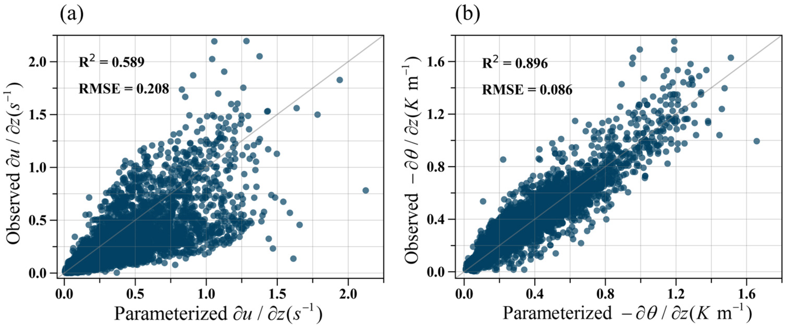
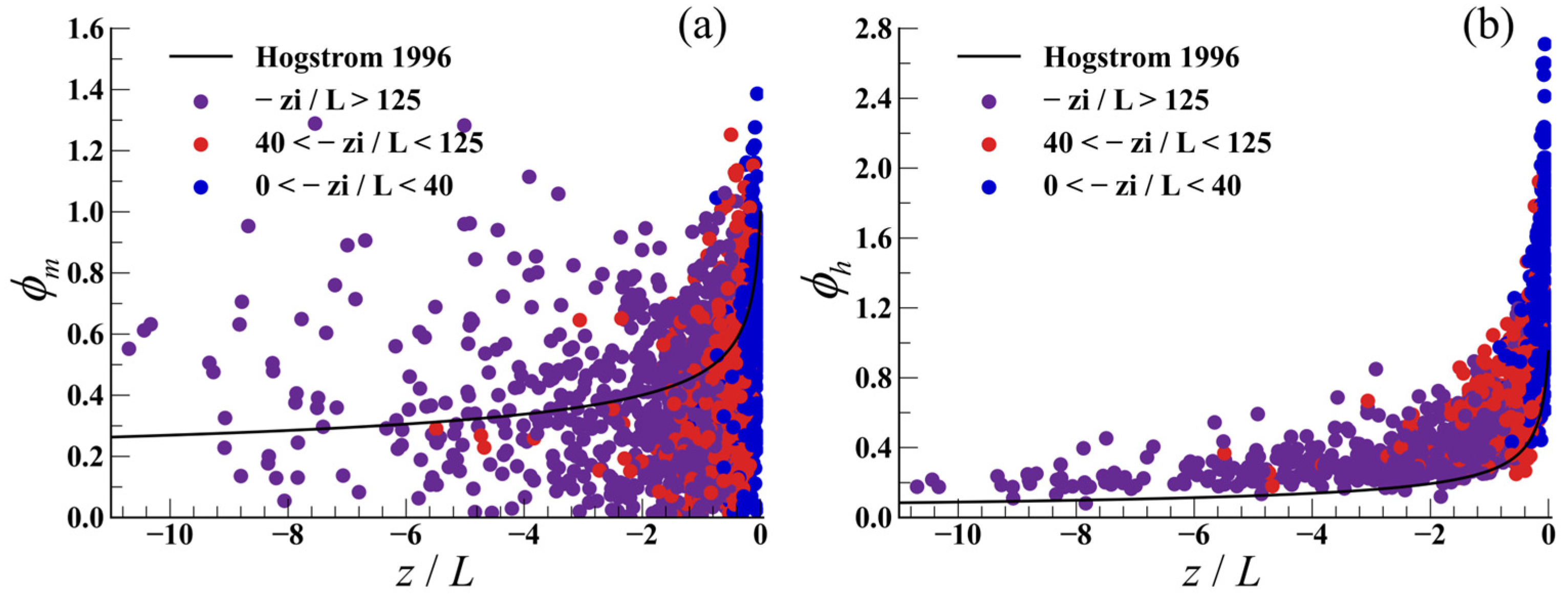
3.3. Nondimensional Flux-Gradient Relations in the Unstable Surface Layer over the Tibetan Plateau

A review of previous studies reveals that there is considerable deviation in the application of the similarity theory for unstable conditions, particularly concerning the mean wind gradient [7,8,9,12,19,30]. In this study, we determine the vertical gradients of the mean wind and temperature directly from observational data by calculating their derivatives (i.e., $du/dz$ for wind and $d\theta /dz$ for temperature). Subsequently, we compare the observational gradients with the values derived from Equations (2) and (3), in which the non-dimensional gradients ($\varphi$) are substituted by the flux-gradient relations given in Equations (8) and (9) for the mean wind and temperature, respectively. According to Table 1, measurements of wind speed and temperature from the Seng-ge Kamba station at 1, 2, 4, 8, and 19 m, as well as those from the Nagqu station at 0.75, 1.5, 3, 6, and 12 m, were utilized to compute the vertical gradients. In practice, if $u_1$ and $u_2$ represent the wind speeds recorded at heights $z_1$ and $z_2$ respectively, then the observational wind speed gradient ${\displaystyle \frac{\partial u}{\partial z}}$ can be calculated as ${\displaystyle \frac{\partial u}{\partial z}}={\displaystyle \frac{u_2-u_1}{z_2-z_1}}$. The predicted gradients are derived based on Monin–Obukhov similarity theory. First, we use the definition of the Obukhov length (Equation (1)) to compute the dimensionless stability parameter $z/L$. Here, z is taken as the intermediate height between the two sensors, i.e., $z={\displaystyle \frac{z_1+z_2}{2}}$. Once $z/L$ is obtained, we apply the corresponding universal functions to determine the predicted gradients (Equations (8) and (9)). This comparison serves to assess the precision and consistency of the flux-gradient relations in estimating surface flux.

As shown in Figure 5a, the vertical gradient of horizontal wind ($\partial u/\partial z$) data exhibits considerable scatter, with a coefficient of determination ($R^2$) of 0.589 and a root mean square error (RMSE) of 0.208. These values indicate a significant discrepancy between the observed and predicted gradients, suggesting that while the flux-gradient relations offer a reasonable approximation, substantial scatter remains in the data. Relative to the wind gradient, the temperature gradients show less scatter (Figure 5b), with an RMSE of approximately 0.086, significantly lower than that of the wind gradient. However, at higher temperature gradient ($\partial \theta /\partial z$) values, greater scatter is observed, likely resulting from the enhanced sensitivity of the gradient to local temperature fluctuations and changes in surface conditions. The gradients of scalar quantities, such as horizontal wind and temperature, generally exhibit substantial scatter, particularly in the case of wind gradients. This scatter tends to increase with larger gradient magnitudes. One plausible explanation is that, under strong convective conditions, the turbulence is increasingly dominated by convective eddies. The standard MOST parameterization, which relies on similarity theory, does not explicitly account for convective velocity scales or the mixed layer depth. As a result, MOST may underestimate the turbulent mixing in cases where these convective effects are significant, leading to the observed discrepancies. This suggests that incorporating additional convective parameters into the flux–gradient formulations could potentially reduce the errors observed for larger gradients.

To minimize the influences of surface roughness on the flux-gradient relations, we excluded the three lowest measurement heights on the tower, which are more susceptible to surface roughness. In this study, we focused on gradient levels taken at 13 m at Seng-ge Kambab and 9 m at Nagqu, which offer a more reliable representation of the flux-gradient relations in the unstable surface layer. Several studies [31,32] support the use of a linear growth model for the convective boundary layer during the morning and midday. However, due to the rapid collapse of the convective boundary layer in the late afternoon and the subsequent formation of a nocturnal stable layer with residual turbulent plumes, a linear decay model is inadequate. Accordingly, our analysis is limited to instances where the boundary layer height exhibits a continuous increase between 08:00 and 20:00 BJT, for which we perform linear interpolation using 30-min intervals.

According to the similarity theory, the dimensionless wind gradient should be a function only of the stability parameter $z/L$. However, as noted in the introduction, there is significant scatter among the various experimental measurements of ${\varphi }_m$. Figure 6 presents a plot of the experimental measurements of ${\varphi }_m$ and ${\varphi }_h$ at Seng-ge Kambab and Nagqu. Additionally, the curve representing the empirical function proposed by [6] is included. The ${\varphi }_m$ data from all measurements exhibit considerable scatter and suggest steeper gradients compared to the empirical function (Figure 6a), which aligns with the findings from previous numerical studies [11,19,25]. The dimensionless temperature gradient ${\varphi }_h$ data (Figure 6b) exhibit a more coherent collapse onto a single curve and present a notably smaller degree of dispersion compared to the corresponding ${\varphi }_m$, which supports the results of earlier numerical studies [8,11,33] and field observations [12,24]. The observed discrepancy can be attributed to the fact that similarity theory yields less accurate predictions for wind speed compared to temperature.

The above analysis indicates that the conventional MOST fails to provide an accurate description of the flux-gradient relations observed in the unstable surface layer, especially for horizontal wind. Previous LES studies [8,24] suggest that ${\varphi }_m$ is expected to exhibit a dependence on both $z/L$ and $z_i/L$. To clearly identify the potential impacts of $z_i/L$, the data are grouped into three separate stability ranges: $0<-z_i/L<40$,$40<-z_i/L<125$ and $-z_i/L>125$. For clarity of analysis, data points corresponding exactly to $-z_i/L=40$ and $-z_i/L=125$ have been excluded, ensuring that the three ranges (0–40, 40–125, and >125) are mutually exclusive. The new ${\varphi }_m$ subsets are plotted against $z/L$ in Figure 7a, with different colors representing data from each of the three $z_i/L$ groups (see the figure legend for details). Although there is considerable scatter within the data in each $z_i/L$ stability group, the data points are clearly clustered into three distinct groups corresponding to the $z_i/L$ ranges of 0–40, 40–125, and >125. This clear segregation indicates that the flux–gradient relationships differ significantly across these stability regimes. Furthermore, the three sets of data remain separated at lower $-z/L$, which corresponds to milder unstable conditions. This general trend is in agreement with previous studies [24]. Figure 7b shows a plot of ${\varphi }_h$ against $z/L$ from the present dataset, together with the expression recommended by [6]. In comparison to ${\varphi }_m$ in Figure 7a, the much lower level of scatter for ${\varphi }_h$ is immediately apparent. Additionally, ${\varphi }_h$ shows a slight ordering with $z_i/L$, although it is less clear than for ${\varphi }_m$. In general, both ${\varphi }_m$ and ${\varphi }_h$ show a certain degree of dependence on $z_i/L$. Consequently, it is crucial to incorporate $z_i/L$ into the parameterization of similarity theory.

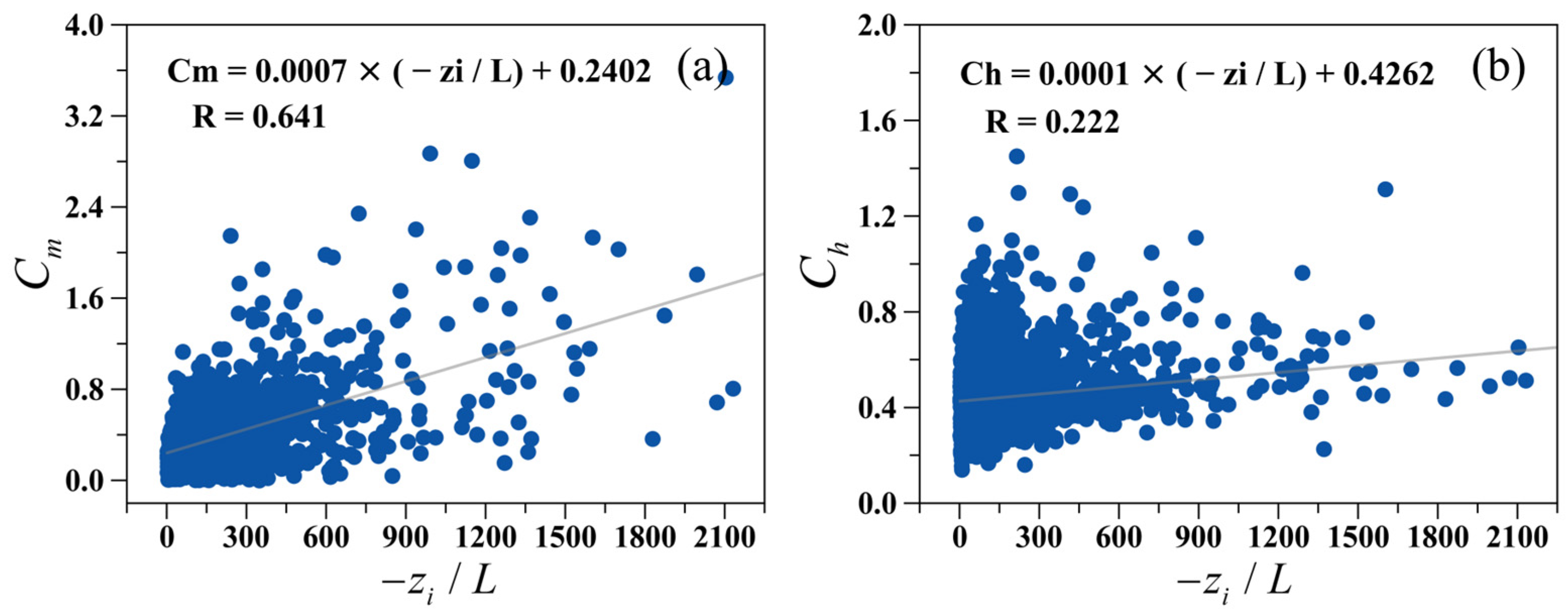
3.4. Factors Influencing Classical Flux-Gradient Relations

Across all 30-min samples, unstable conditions over a broad range of $z_i/L$ are considered for analysis. These results correspond to convective boundary layer heights ($z_i$) between 0 and 3000 m and Obukhov lengths ($L$) between −1 and −200 m. The analysis in Section 3.3 demonstrates that the profiles of wind and temperature under unstable conditions are closely related to the parameter $z_i/L$, where $z_i$ is a scaling parameter representing large eddies. To account for the effect of large convective eddies, an improved universal function using the scaling parameter $z/z_i$ was introduced in [25], as shown in Equation (10). However, this scheme is constrained by its in ability to accurately determine the parameter $\alpha$ in applications, which represents the ratio of $z_i$ to the height where heat flux vanishes, especially in observational analysis and offline simulations of surface models. The improved flux-gradient relations were assessed in [34] using LES data from [25], and it was found that omitting the parameter $\alpha$ leads to a new scheme:

$${\varphi }_m=C_m{(-{\displaystyle \frac{z}{L}})}^{-1/2}$$

(12)

where $C_m$ could further be expressed as

$$C_m=0.0047(-{\displaystyle \frac{z_i}{L}})+0.1854$$

(13)

Since LES data demonstrate that $C_m$ holds a significant linear relationship with $-z_i/L$, we now investigate whether this linear relationship also holds for the TIPEX-III dataset. For unstable conditions, we calculated $C_m$ using Equation (12), where ${\varphi }_m$ is obtained from the observation measurements (Equation (2)):

$$C_m={\displaystyle \frac{{\varphi }_m}{{(-\frac{z}{L})}^{-1/2}}}$$

(14)

Based on the data points in Figure 8a, we infer that the linear relationship between $C_m$ and $-z_i/L$ is reasonable, giving $C_m=0.0007\times (-z_i/L)+0.2402$ with a correlation coefficient (R) of 0.641. Despite the higher uncertainty in the observational data, these results suggest that a linear trend remains plausible. Similarity, we derive $C_h$ as a function of ${\varphi }_h$ and $-z/L$:

$$C_h={\displaystyle \frac{{\varphi }_h}{{(-\frac{z}{L})}^{-1/2}}}$$

(15)

It is difficult to discern a consistent linear relationship between $C_h$ and $-z_i/L$, as indicated by a correlation coefficient of 0.222 (Figure 8b).

Table 2. General form of universal function.

Reference	Universal Form
Hogstrom 1988 [5]	$1.0{(1-15.2{\displaystyle \frac{z}{L}})}^{-1/4}$
Dyer 1974 [3]	$1.0{(1-16.0{\displaystyle \frac{z}{L}})}^{-1/4}$
Högström (1996) [6]	$1.0{(1-19.0{\displaystyle \frac{z}{L}})}^{-1/4}$
This study (new power law)	${(-{\displaystyle \frac{z}{L}})}^{-1/2}$
New power law 1	${(-{\displaystyle \frac{z}{L}})}^{-1/3}$
New power law 2	${(-{\displaystyle \frac{z}{L}})}^{-1/4}$

compares the universal functional forms from earlier investigations with the new power law proposed by [34], which employs a slope of −1/2. In addition, slopes of −1/3 and −1/4 are included for reference. Based on the LES analyses [34], the −1/2 scaling more effectively captures the behavior of turbulent fluxes in the atmospheric boundary layer, which justifies our adoption of the new power law and the corresponding $C_m$ functions. It should be noted that we examine three distinct universal forms of: (1) the conventional form based on traditional MOST relations [3,5,6]; (2) the improved similarity relationship derived from LES data, as proposed by [34]; and (3) the transformed form derived from the LES-based universal form. In this study, we obtain parameter $C_m$ following Equation (14) where the ${(-{\displaystyle \frac{z}{L}})}^{-1/2}$ term in the equation is replaced with 6 different forms as presented in Table 2. We then examine the relationship between $C_m$ and $-z_i/L$ (Figure 9). $C_m$ derived from the new universal form suggested by [34] shows a significant linear relationship with $-z_i/L$, with a correlation coefficient (R) as high as 0.641 (Figure 9d). In contrast, Cm derived from the traditional form based on MOST relations (Figure 9a–c) fails to reproduce this linear relationship. These results show that the relationship between $C_m$ and $-z_i/L$ obtained based on the empirical MOST form is not obvious. Moreover, no consistent relationship between $C_m$ and $-z_i/L$ is observed in the transformed supplementary universal forms with slope of −1/3 and −1/4 (Figure 9e,f). Therefore, we must admit that relationship between $C_m$ and $-z_i/L$ is not well captured by the empirical MOST formulations in comparison with new fitting function proposed by [34].

In this study, we derived the relationship between $C_m$ and $-z_i/L$, expressed as $C_m=0.0007\times (-z_i/L)+0.2402$ (see Figure 9d). Based on this, the revised universal function ${\varphi }_m$ was determined using the relation ${\varphi }_m=C_m{(-z/L)}^{-1/2}$. The derived ${\varphi }_m$ was then employed to calculate the vertical gradient of horizontal wind speed ($\partial u/\partial z$), which was subsequently compared with the observed gradient (see Figure 10). As illustrated in Figure 10, the coefficient of determination ($R^2$) between the observed and parameterized vertical wind gradients is 0.582, with an RMSE of 0.024. Although this revised scheme yields a slightly lower $R^2$ compared to the classical universal function ($R^2=0.589$, RMSE = 0.208; see Figure 5a), the significantly reduced RMSE demonstrates a clear advantage in prediction accuracy.

Physically, friction velocity and momentum flux quantify the exchange of momentum between the surface and the lower atmosphere, while sensible heat flux describes the transfer of heat near the surface—both being crucial metrics in boundary-layer meteorology. In this work, we further compare the friction velocity, momentum flux, and sensible heat flux computed using the classical universal function introduced by [6], referred to hereafter as the MOST scheme, and the revised universal function presented by [25], hereafter the LZD scheme, against observed data (Figure 11). The results indicate that at Seng-ge Kamba station and Nagqu station, predictions of friction velocity and momentum flux by the MOST scheme fall below the observed values (Figure 11a–d). By contrast, the LZD scheme closely approximates the measurements, representing a significant improvement over MOST. For sensible heat flux, the MOST scheme tends to overestimate the observed values. Since the LZD scheme predicts a higher friction velocity, its corresponding sensible heat flux is also greater (Equation (5)). Overall, the vertical wind speed gradient predicted by the LZD scheme exhibits a smaller root mean square error (RMSE) than that of the MOST scheme, indicating reduced prediction bias. Moreover, friction velocity and momentum flux obtained from the LZD scheme align better with observations.

4. Conclusions and Discussion

Using field data from two intensive summer field campaigns on the Tibetan Plateau, which include turbulence measurements, profile data, and boundary layer height observations, we investigated the impact of large eddies in the surface layer. Our findings provide evidence supporting the crucial role of boundary layer height ($z_i$) in surface flux parameterization, which is a scaling variable for large eddies. Furthermore, we evaluate the applicability of the improved similarity function proposed by [25] to the unstable surface layer, where it accounts for the large eddy effects in surface flux parameterization. Based on our analysis of the proposed scheme, we suggest that it can be simplified to enhance its applicability for Earth system modeling. Finally, we applied the proposed similarity function to derive the associated surface flux quantities and observed that it displays promising feasibility for practical implementation.

The non-dimensional wind shear, ${\varphi }_m$, in the surface layer demonstrates more scatter and a stronger deviation from the Monin-Obukhov similarity theory (MOST) compared to the non-dimensional temperature gradient, ${\varphi }_h$, under unstable surface layer conditions, which aligns with the findings from previous numerical studies [11,24,33]. On the other hand, the non-dimensional temperature gradient, ${\varphi }_h$, shows less scatter and generally conforms to MOST, consistently with prior research, which supports the results of earlier numerical studies [8,11,33] and field observations [12,24]. In addition to its expected relationship with $z/L$ in classical similarity theory, the non-dimensional wind gradient, ${\varphi }_m$, demonstrates a clear dependence on the stability parameter $z_i/L$. Conversely, ${\varphi }_h$ shows a weaker dependence on $z_i/L$, although this effect is less pronounced than for ${\varphi }_m$. These findings align with [8,24,25], implying that $z_i/L$ might serve as the missing scaling parameter in MOST under unstable conditions.

In the TIPEX-III dataset, the $z_i$-scaling parameter $C_m$ derived from the proposed scheme demonstrates a robust linear correlation with the stability parameter $-z_i/L$, further validating the feasibility of the scheme. We further evaluated the wind speed gradient, friction velocity, momentum flux, and sensible heat flux generated using the classical universal function and revised universal function proposed by [25], benchmarking each against field observations. The revised formulation achieves a lower root mean square error (RMSE) than the MOST framework for the vertical wind speed gradient, indicating less bias. Its predicted friction velocity and momentum flux also align better with measured values. Taken together, these results verify the validity of our approach while suggesting simplifications that enhance its applicability to Earth system modeling.

It is evident from our results that deviations of ${\varphi }_m$ from the Monin-Obukhov similarity theory (MOST) under unstable stratification are systematically influenced by the candidate $z_i/L$ values derived from our field measurements. This outcome implies that $z_i/L$ not only captures large-eddy effects but may also serve as a meaningful additional parameter for refining surface-layer similarity functions. In particular, our findings suggest that properly incorporating $z_i/L$ could help account for large eddy influences, which are often neglected in conventional surface-layer scaling but appear crucial when instability is significant. However, despite the observed correlation, our current dataset and analyses do not yet allow us to definitively establish a precise formulation for the dimensionless wind gradient, ${\varphi }_m$. Variations in surface roughness, thermal stratification, and measurement conditions all introduce uncertainties that make it challenging to propose a universal expression at this stage. To address these uncertainties, we plan to conduct further research by combining additional field campaigns covering diverse terrain types and atmospheric conditions with high-resolution large-eddy simulations. Such an integrated approach will enable us to more thoroughly evaluate the robustness and generalizability of any revised universal similarity function, thereby ensuring that the role of $z_i/L$ is accurately captured. Despite these current limitations, our work offers new insights into how the inclusion of $z_i/L$ can improve the predictive accuracy of turbulence models in boundary-layer studies. By highlighting the systematic influence of $z_i/L$ on surface-layer dynamics, we underscore the potential of this parameter to bridge gaps in existing similarity theories, particularly in strongly unstable regimes where large-eddy motions dominate. With further validation and refinement, the approach presented here has the potential to enhance the representation of near-surface turbulent fluxes in Earth system models, ultimately contributing to more accurate forecasts of weather and climate processes.

References

1. Monin, A.S.; Obukhov, A.M. Basic Laws of Turbulent Mixing in the Atmospheric Surface Layer. Contrib. Geophys. Inst. Slovak Acad. Sci. 1954, 24, 163–187. [Google Scholar]
2. Businger, J.A.; Wyngaard, J.C.; Izumi, Y.; Bradley, E.F. Flux-profile relationships in the atmospheric surface layer. J. Atmos. Sci. 1971, 28, 181–189. [Google Scholar] [CrossRef]
3. Dyer, A.J. A Review of Flux-Profile Relationships. Bound.-Layer Meteorol. 1974, 7, 363–372. [Google Scholar] [CrossRef]
4. Panofsky, H.A.; Dutton, J.A. Atmospheric Turbulence; John Wiley & Sons: New York, NY, USA; Chichester, UK; Toronto, ON, Canada; Singapore, 1984. [Google Scholar]
5. Hogstrom, U. Non-dimensional Wind and Temperature Profiles in the Atmospheric Surface Layer: A Re-Evaluation. Bound.-Layer Meteorol. 1988, 42, 55–78. [Google Scholar] [CrossRef]
6. Hogstrom, U. Review of Some Basic Characteristics of the Atmospheric Surface Layer. Bound.-Layer Meteorol. 1996, 78, 215–246. [Google Scholar] [CrossRef]
7. Panofsky, H.A.; Tennekes, H.; Lenschow, D.H.; Wyngaard, J.C. The Characteristics of Turbulent Velocity Components in the Surface Layer under Convective Conditions. Bound.-Layer Meteorol. 1977, 11, 355–361. [Google Scholar] [CrossRef]
8. Khanna, S.; Brasseur, J.G. Analysis of Monin–Obukhov similarity from large-eddy simulation. J. Fluid Mech. 1997, 345, 251–286. Available online: https://ui.adsabs.harvard.edu/abs/1997JFM...345..251K/abstract (accessed on 10 November 2024).
9. Katul, G.G.; Konings, A.G.; Porporato, A. Mean Velocity Profile in a Sheared and Thermally Stratified Atmospheric Boundary Layer. Phys. Rev. Lett. 2011, 107, 268502. [Google Scholar] [CrossRef]
10. Banerjee, T.; Li, D.; Juang, J.; Katul, G. A spectral budget model for the longitudinal turbulent velocity in the stable atmospheric surface layer. J. Atmos. Sci. 2016, 73, 145–166. [Google Scholar] [CrossRef]
11. Li, Q.; Gentine, P.; Mellado, J.P.; McColl, K.A. Implications of Nonlocal Transport and Conditionally Averaged Statistics on Monin–Obukhov Similarity Theory and Townsend’s Attached Eddy Hypothesis. J. Atmos. Sci. 2018, 75, 3403–3431. [Google Scholar] [CrossRef]
12. Salesky, S.T.; Chamecki, M. Random Errors in Turbulence Measurements in the Atmospheric Surface Layer: Implications for Monin–Obukhov Similarity Theory. J. Atmos. Sci. 2012, 69, 3700–3714. [Google Scholar] [CrossRef]
13. Sorbjan, Z. On similarity in the atmospheric boundary layer. Bound.-Layer Meteorol. 1986, 34, 377–397. [Google Scholar] [CrossRef]
14. Deardorff, J.W. Numerical Investigation of Neutral and Unstable Planetary Boundary Layers. J. Atmos. Sci. 1972, 29, 91–115. [Google Scholar] [CrossRef]
15. Kaimal, J.C.; Wyngaard, J.C.; Izumi, Y.; Coté, O.R. Spectral Characteristics of Surface-Layer Turbulence. Q. J. R. Meteorol. Soc. 1972, 98, 563–589. [Google Scholar] [CrossRef]
16. Steeneveld, G.J.; Holtslag, A.A.M.; Debruin, H.A.R. Fluxes and Gradients in the Convective Surface Layer and the Possible Role of Boundary-Layer Depth and Entrainment Flux. Bound.-Layer Meteorol. 2005, 116, 237–252. [Google Scholar] [CrossRef]
17. McNaughton, K.G. On the Kinetic Energy Budget of the Unstable Atmospheric Surface Layer. Bound.-Layer Meteorol. 2006, 118, 83–107. [Google Scholar] [CrossRef]
18. Gioia, G.; Guttenberg, N.; Goldenfeld, N.; Chakraborty, P. Spectral Theory of the Turbulent Mean-Velocity Profile. Phys. Rev. Lett. 2010, 105, 184501. [Google Scholar] [CrossRef]
19. Katul, G.G.; Li, D.; Chamecki, M.; Bou-Zeid, E. Mean Scalar Concentration Profile in a Sheared and Thermally Stratified Atmospheric Surface Layer. Phys. Rev. 2013, 87, 023004. [Google Scholar] [CrossRef]
20. Gao, Z.; Liu, H.; Russell, E.S.; Huang, J.; Foken, T.; Oncley, S.P. Large Eddies Modulating Flux Convergence and Divergence in a Disturbed Unstable Atmospheric Surface Layer. J. Geophys. Res. Atmos. 2016, 121, 1475–1492. [Google Scholar] [CrossRef]
21. McColl, K.A.; Katul, G.G.; Gentine, P.; Entekhabi, D. Mean-Velocity Profile of Smooth Channel Flow Explained by a Cospectral Budget Model with Wall-Blockage. Phys. Fluids. 2016, 28, 035107. [Google Scholar] [CrossRef]
22. Mellado, J.P.; Van Heerwaarden, C.C.; Garcia, J.R. Near-Surface Effects of Free Atmosphere Stratification in Free Convection. Bound.-Layer Meteorol. 2016, 159, 69–95. [Google Scholar] [CrossRef]
23. Cheng, Y.; Li, Q.; Li, D.; Gentine, P. Logarithmic Profile of Temperature in Sheared and Unstably Stratified Atmospheric Boundary Layers. Phys. Rev. Fluids. 2021, 6, 034606. [Google Scholar] [CrossRef]
24. Johansson, C.; Smedman, A.-S.; Högström, U.; Brasseur, J.G.; Khanna, S. Critical test of the validity of Monin–Obukhov similarity during convective conditions. J. Atmos. Sci. 2001, 58, 1549–1566. [Google Scholar] [CrossRef]
25. Liu, S.; Zeng, X.; Dai, Y.; Shao, Y. Further improvement of surface flux estimation in the unstable surface layer based on large-eddy simulation data. J. Geophys. Res. Atmos. 2019, 124, 9839–9854. [Google Scholar] [CrossRef]
26. Zhao, P.; Xu, X.; Chen, F.; Guo, X.; Zheng, X.; Liu, L.; Hong, Y.; Li, Y.; La, Z.; Peng, H. The Third Atmospheric Scientific Experiment for Understanding the Earth–Atmosphere Coupled System over the Tibetan Plateau and Its Effects. Bull. Am. Meteorol. Soc. 2018, 99, 757–776. [Google Scholar] [CrossRef]
27. Wang, Y.; Xu, X.; Liu, H.; Li, Y.; Li, Y.; Hu, Z.; Gao, X.; Ma, Y.; Sun, J.; Lenschow, D.H.; et al. Analysis of land surface parameters and turbulence characteristics over the Tibetan Plateau and surrounding region. J. Geophys. Res. Atmos. 2016, 121, 9540–9560. [Google Scholar] [CrossRef]
28. Che, J.; Zhao, P. Characteristics of the summer atmospheric boundary layer height over the Tibetan Plateau and influential factors. Atmos. Chem. Phys. 2021, 21, 5253–5268. [Google Scholar] [CrossRef]
29. Liu, S.Y.; Liang, X.Z. Observed diurnal cycle climatology of planetary boundary layer height. J. Clim. 2010, 23, 5790–5809. [Google Scholar] [CrossRef]
30. Katul, G.G.; Porporato, A.; Shah, S.; Bou-Zeid, E. Two phenomenological constants explain similarity laws in stably stratified turbulence. Phys. Rev. E 2014, 89, 023007. [Google Scholar] [CrossRef]
31. Stull, R.B. An Introduction to Boundary Layer Meteorology; Kluwer Academic Publishers: Dordrecht, The Netherlands, 1988. [Google Scholar]
32. Garratt, J.R. The Atmospheric Boundary Layer; Cambridge University Press: Cambridge, UK, 1994. [Google Scholar]
33. Pirozzoli, S.; Bernardini, M.; Verzicco, R.; Orlandi, P. Mixed convection in turbulent channels with unstable stratification. J. Fluid Mech. 2017, 821, 482–516. [Google Scholar] [CrossRef]
34. Liu, S.; Zeng, X.; Dai, Y.; Yuan, H.; Wei, N.; Wei, Z.; Lu, X.; Zhang, S. A Surface Flux Estimation Scheme Accounting for Large-Eddy Effects for Land Surface Modeling. Geophys. Res. Lett. 2022, 49, e2022GL101754. [Google Scholar] [CrossRef]
Figure 1. Geographic locations of the two observation stations (Seng-ge Kambab and Nagqu) on the Tibetan Plateau employed in this study, shown on a terrain-height map (in meters). The color scale ranges from 0 to over 7000 m, highlighting the plateau’s significant topographical gradient. Red stars indicate the station positions, while black lines delineate major contour intervals. Latitude and longitude are labeled along the figure’s axes for reference.
Atmosphere 16 00391 g001
Figure 2. Diurnal variation of (a) momentum flux ( τ ), (b) sensible heat flux (SHF), and (c) latent heat flux (LHF), averaged over the study period at Seng-ge Kambab and Nagqu. The period from 08:00 to 20:00 is shaded in gray to denote daylight hours on the Tibetan Plateau.
Atmosphere 16 00391 g002
Figure 3. Time series of the absolute value of the Obukhov length ( L ), averaged over the study period at Seng-ge Kambab and Nagqu.
Atmosphere 16 00391 g003
Figure 4. Diurnal variations in planetary boundary layer height (PBLH) and sensible heat flux (SHF) measured at two locations: Seng-ge Kambab (SQH, red) and Nagqu (NQ, blue), on three selected days: (a) 23 June 2015, (b) 29 June 2015, and (c) 2 July 2015. The PBLH is shown by colored bars, and the SHF is represented by the solid line with circles.
Atmosphere 16 00391 g004
Figure 5. Comparison of the observed gradient and the parameterized gradient from the classical universal functions suggested by [6]: (a) horizontal wind gradient ( u / z ), and (b) temperature gradient ( θ / z ).
Atmosphere 16 00391 g005
Figure 6. Plot of (a) dimensionless wind gradient ϕ m and (b) temperature gradient ϕ h versus the stability parameter z / L for all measurements. Solid line: empirical curve from [6].
Atmosphere 16 00391 g006
Figure 7. Plot of (a) dimensionless wind gradient ϕ m and (b) temperature gradient ϕ h versus the stability parameter z / L for all measurements across three z i / L ranges: purple dots: z i / L > 125 , red dots: 40 < z i / L < 125 and blue dots: 0 < z i / L < 40 . Solid line: empirical curve from [6].
Atmosphere 16 00391 g007
Figure 8. (a) C m and (b) C h versus z i / L . Solid line: linear regression of C m and C h versus z i / L . The correlation coefficient (R) is given in each panel.
Atmosphere 16 00391 g008
Figure 9. Plot of C m versus z i / L estimated using different universal forms: (a) Dyer (1974) [3], (b) Panofsky and Dutton (1984) [4], (c) Högström (1996) [6], (d) ( z L ) 1 / 2 , (e) ( z L ) 1 / 3 , and (f) ( z L ) 1 / 4 . Solid line: curve fitted to the data.
Atmosphere 16 00391 g009
Figure 10. Comparison of the observed vertical wind gradient ( u / z ) with the gradient parameterized using the revised universal functions proposed by [25].
Atmosphere 16 00391 g010
Figure 11. Diurnal variations (08:00–20:00 BJT) of friction velocity, momentum flux, and sensible heat flux at Seng-ge Kamba station (subplots (a,c,e)) and Nagqu station (subplots (b,d,f)). The figure compares variables derived from observational data (OBS), the classic universal function (MOST) proposed by [6], and the revised function (LZD) introduced by [25].
Atmosphere 16 00391 g011