Summer Diurnal LST Variability Across Local Climate Zones Using ECOSTRESS Data in Lecce and Milan

Abstract

This study assesses the accuracy of Local Climate Zone (LCZ) classification and its impact on land surface temperature (LST) analysis in Mediterranean cities using high-resolution ECOSTRESS data. Two classification methods were compared: a Geographic Information System (GIS)-based approach integrating high-resolution geospatial data and an LCZ map derived from WUDAPT. Discrepancies in LCZ classification influenced the spatial distribution of urban forms, with WUDAPT overestimating LCZ 6 (open low-rise) and LCZ 8 (large low-rise) while underrepresenting more compact urban types. LST analysis revealed distinct thermal responses between Milan and Lecce, underscoring the influence of urban morphology and local climate. Densely built zones (LCZ 2, LCZ 5) exhibited the highest temperatures, especially at night, while LCZ 8 also retained significant heat. Milan’s dense urban areas experienced pronounced nighttime overheating, whereas Lecce showed a clear daytime temperature gradient, with historic districts (LCZ 2) maintaining lower LST the light-colored and high thermal capacity of building materials. A Kruskal–Wallis test confirmed significant differences between the GIS-based and WUDAPT-derived LCZ maps, highlighting the impact of classification methodology and spatial resolution on LST analysis. These findings emphasize the need for multi-scale approaches to urban climate adaptation and mitigation, providing valuable advice for urban planners and policymakers in development of sustainable and climate-resilient cities. This research is also among the first to integrate ECOSTRESS data with LCZ maps to examine LST variations across spatial and temporal scales.

1. Introduction

Urban planning and sustainable development are essential for enhancing the resilience and well-being of cities, particularly in the face of climate change and rapid urbanization. A comprehensive understanding of the interactions between climatic conditions and the urban microclimate is crucial for improving air quality and thermal environments [1]. The Local Climate Zone (LCZ) classification system plays a key role in this process by systematically categorizing urban areas based on their climatic and physical attributes [2,3]. The LCZ methodology provides a structured framework for urban planners to analyze distinct climate profiles within cities. Through LCZ classification, areas vulnerable to extreme temperatures, air pollution, or other environmental stressors can be identified, enabling targeted interventions to enhance climate resilience and urban living [4].

Analyzing local climate patterns has broader implications for sustainable urban development. Detailed climate data help identify opportunities to integrate green infrastructure, such as urban forests, green roofs, and permeable surfaces, which mitigate the Urban Heat Island (UHI) effect, improve air quality, enhance biodiversity, and promote the well-being of urban populations [5].

Additionally, the LCZ classification system facilitates intercity and interregional comparisons, fostering knowledge exchange among cities to address common urban challenges, such as rising temperatures, air pollution, and energy consumption. LCZ classifications serve as a foundation for implementing effective mitigation and adaptation strategies. Cities with similar LCZ patterns can share best practices in green space management or urban energy efficiency, accelerating progress toward urban sustainability [6].

In this context, this study aims to evaluate the accuracy and applicability of LCZ classifications in urban climate research. Specifically, it presents a comparative analysis of LCZs using geographic information systems (GIS) and morphological data to classify LCZs across several Italian cities located in the southern, central, and northern regions. A key component of this research is the comparison between two LCZ mapping approaches: a GIS-based LCZ map (hereinafter GIS-based map) and the European LCZ Level 0 map (hereinafter WUDAPT European LCZ map) developed by Demuzere et al. [6] is available as a downloadable GeoTIFF file from the World Urban Database and Access Portal Tools (WUDAPT) from which the city area of interest has been cropped. (https://figshare.com/articles/dataset/European_LCZ_map/13322450, last accessed 2 May 2025). According to their methodology, the validation was carried out through a comprehensive accuracy assessment, which involved a bootstrap cross-validation technique. In this process, the dataset was repeatedly sampled to evaluate the model’s performance. Additionally, thematic benchmarks for 150 selected functional urban areas were established using independent global and open-source data on surface cover, surface imperviousness, building height, and anthropogenic heat [6,7]

The spatial distribution of heat in urban areas has traditionally been assessed through fixed-point air temperature measurements, satellite-based land surface temperature (LST) data [8,9,10,11], and numerical modeling. Extensive research has explored urban heat and evaluated the effectiveness of various mitigation strategies across different cities. Many studies utilize satellite-derived land surface temperature (LST) to analyze urban heat patterns from a broad, top-down perspective. The widespread use of LST data in heat mitigation studies is driven by its ability to provide consistent, global-scale observations of land surface temperatures through satellite monitoring [12,13]

Despite the availability of multiple remote sensing datasets, capturing diurnal variations in LST or Surface Urban Heat Island (SUHI) at a high spatial resolution remains a challenge. While satellites such as MODIS and Sentinel-3 provide frequent daily LST data [14,15,16], their relatively coarse spatial resolution (1 km²) limits their effectiveness for urban microclimate studies. Similar studies such as Wu et al. [17] have characterized the spatial heterogeneity of the urban thermal environment at the city level using LSTs retrieved from Landsat-8. Higher-resolution satellites like Landsat or ASTER enable more precise spatial analyses but suffer from temporal limitations. However, ASTER provides only a limited number of images per city, while Landsat acquires data at fixed intervals and lacks nighttime observations [18,19].

To address these limitations, this study integrates high-resolution thermal data from the Ecosystem Spaceborne Thermal Radiometer Experiment on Space Station (ECOSTRESS) into urban temperature analyses.

This study assesses surface temperature patterns across different cities using ECOSTRESS satellite data. The analysis builds upon the previous objective by utilizing the two LCZ classifications described earlier (WUDAPT European LCZ and GIS-based maps). Integrating these datasets enables an evaluation of how different LCZ classification methods influence the assessment of the urban thermal environment. Additionally, a detailed examination of thermal variations across LCZs serves as a key indicator of the reliability and representativeness of the chosen classification approach.

The potential of ECOSTRESS for capturing diurnal LST variability has been highlighted in studies such as Chang et al. [20], Chang et al. [21], Hulley et al. [22], and Wei et al. [23]. Launched aboard the International Space Station (ISS) on 29 June 2018, ECOSTRESS provides LST observations with a high spatial resolution of 70 × 70 m, capturing thermal data at different times of day and night based on local time (LT), improving the temporal characterization of urban thermal environments [24].

The novelty of this study lies in its medium-to-long-term analysis of ECOSTRESS data, distinguishing it from prior research that primarily focused on short-term periods. For example, Chang et al. [20] examined ECOSTRESS LST data only between 1 June and 30 September 2019. In contrast, this study utilizes ECOSTRESS LST data for the summer months (June, July, and August, hereinafter JJA) from 2018 to 2024, combining them with LCZ maps to analyze diurnal LST dynamics in Lecce (a small city in southern Italy) and Milan (a metropolis in northern Italy). By leveraging ECOSTRESS’s unique ability to capture LST variations at different times of the day over multiple years, this study provides a comprehensive assessment of the diurnal thermal behavior based on robust statistical analysis.

Advanced statistical techniques are employed to assess the significance of the data and to identify similarities among different LCZs in Lecce and Milan across various time periods. The findings contribute to a deeper understanding of the relationship between urban form and thermal dynamics, supporting urban planners and policymakers in developing climate adaptation and mitigation strategies.

This research provides essential knowledge into the role of LCZ mapping in shaping future urban growth and regeneration efforts. As urban areas continue to expand, integrating climate-sensitive planning approaches is critical to mitigating environmental stressors. LCZ data facilitate the identification of priority areas for climate adaptation measures, including increasing vegetation cover, improving energy efficiency, and optimizing road networks to enhance air circulation [25]. Ultimately, this study underscores the importance of incorporating high-resolution LST data into urban climate research to support sustainable development and urban resilience [26].

2. Methodology

2.1. Study Areas

This study focuses on five Italian cities—Bari, Naples, Rome, Milan, and Lecce. The selection includes four major metropolitan cities (Bari, Naples, Rome, and Milan) representing different regions of Italy (south, center, and north). In addition, Lecce was included because of its association with the University of Salento.

The selected cities include different climatic conditions according to Köppen’s classification. Naples, Rome, and Lecce share a Mediterranean climate (Csa), characterized by mild winters and hot, dry summers. Bari, on the other hand, has a humid subtropical climate (Cfa), characterized by relatively high temperatures and evenly distributed precipitation throughout the year. Milan, located in northern Italy, falls into the category of west coast marine climate (Cfb), characterized by moderate temperature variations and consistent precipitation throughout the seasons (source: https://koeppen-geiger.vu-wien.ac.at/, accessed 19 December 2024).

Regarding urban development, Milan is the largest among these cities, exhibiting a radial expansion pattern with new districts emerging outward from the historical core. Rome similarly follows a radial growth model but features multiple urban centers interspersed with significant green areas. Lecce also expands radially, with its urban growth directed northwest toward the industrial sector, east toward the coast, and south in predominantly residential zones. As coastal cities, Naples and Bari have distinct development patterns: Naples has expanded along the shoreline, influenced by the presence of Mount Vesuvius, whereas Bari has grown further inland (Figure 1).

2.2. Collecting Morphological Data

Morphological and land use data were collected and analyzed using shapefiles for all cities. The data were obtained from the following institutional sources:

• for Lecce and Bari, SIT Puglia (http://www.sit.puglia.it, last accessed on 14 April 2022);
• for Naples, Geoportale Nazionale (http://wms.pcn.minambiente.it, last accessed on 18 May 2022);
• for Rome Open Data Lazio (https://geoportale.regione.lazio.it, last accessed on 20 October 2022);
• for Milan, Milano Geoportale (https://geoportale.comune.milano.it, last accessed on 17 June 2022).

2.3. Estimation of Morphological Parameters Using GIS

A morphological analysis was performed using QGIS software (version: 3.22.1, https://www.qgis.org/en/site, accessed on 10 December 2024). A region of interest (ROI) was defined for each selected city, with its dimensions adjusted based on the city’s size. Specifically, a 10 km × 10 km area was designated for Lecce and Bari (hereafter referred to as the “Lecce region” and “Bari region”), while a larger 20 km × 20 km area was allocated for Naples, Rome, and Milan (hereafter the “Naples region,” and so forth).

The analysis included key urban canopy parameters (UCPs) such as mean building height, sky view factor, aspect ratio, building surface fraction, and the fractions of impervious and permeable surfaces. These parameters were computed at a spatial resolution of 100 m × 100 m following the classification framework proposed by Stewart and Oke [2]. For a comprehensive explanation of the calculation methodology, refer to Esposito et al. [27]. 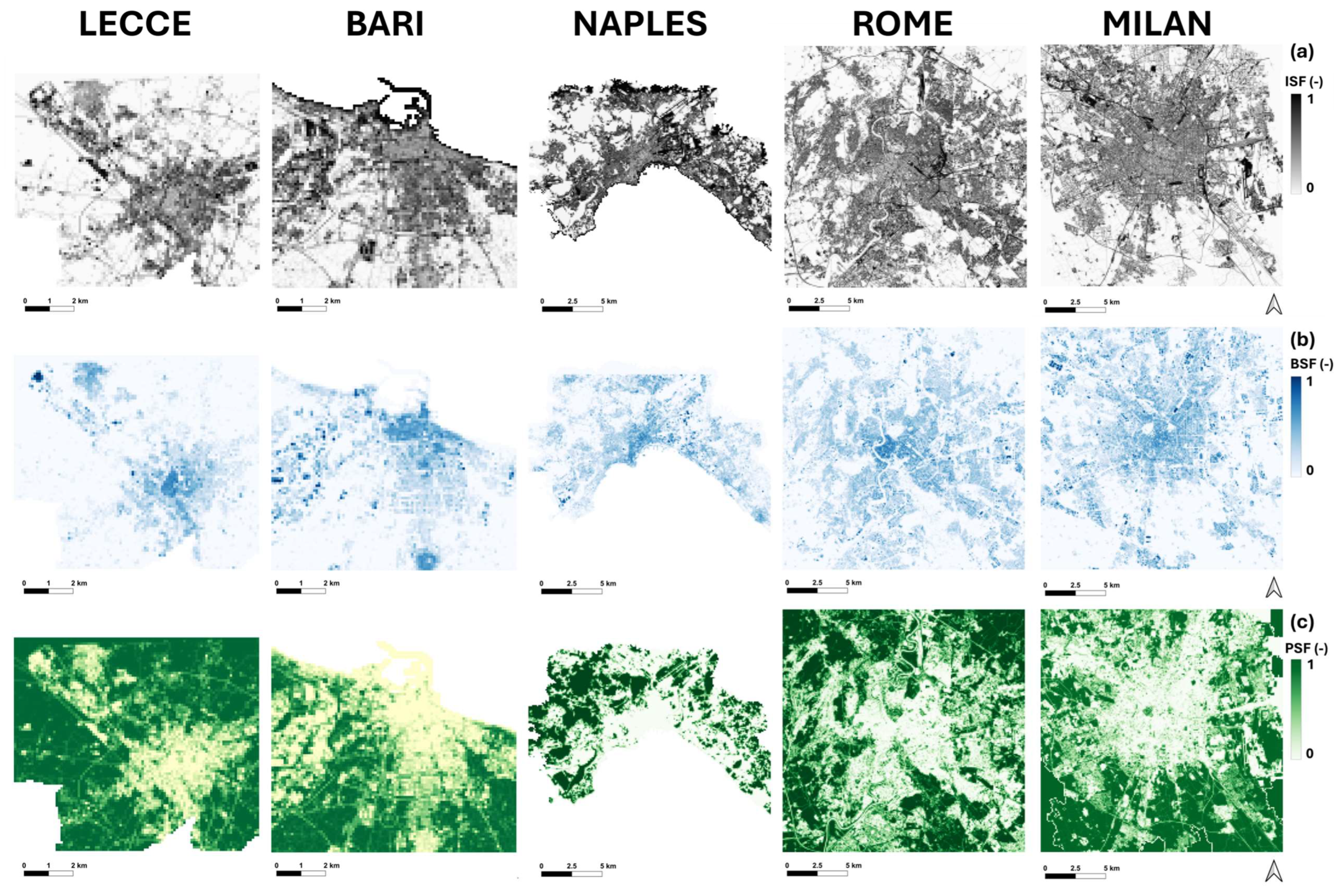Regarding the building surface fraction (BSF), fraction of impervious surface (ISF) and permeable surface (PSF), Stewart and Oke [2] describe them respectively as the ratio of building plan area, the ratio of impervious surface (paved, rocks, roads, etc.) to total area (%) and as the ratio of permeable surface (bare soil, vegetation, water, green space, agricultural land, etc.) to total area (%).

In calculating these parameters, the sum of ISF, PSF, and BSF values in a single grid cell are equal to 1, so in the absence or lack of permeable elements for PSF calculation, a simple subtraction was performed to obtain this parameter:

$$\mathrm{P}\mathrm{S}\mathrm{F}=1-(\mathrm{B}\mathrm{S}\mathrm{F}+\mathrm{I}\mathrm{S}\mathrm{F})$$

(1)

Figure 2 shows the maps of the PSF, ISF, and BSF parameters of all cities at a spatial resolution of 100 × 100.

All the cities show an urban center with prevalence of areas with both high BSF values (generally between 0.70 and 0.95) and high ISF values, underscoring the prevalence of impervious areas (roads, sidewalks and squares) and low PSF values, which instead shows a tendency to increase moving outward from the cities.

2.4. Construction of the GIS-Based Maps

The creation of GIS-based maps involved calculating the actual morphological parameters of a city and applying fuzzy logic to improve classification accuracy. This approach integrates geometric and surface coverage properties, including sky view factor (SVF), BSF, ISF, aspect ratio (AR), and average building height (HM), to classify urban and rural areas into distinct LCZs [28] based on Stewart and Oke’s criteria [2]. The map was constructed by assigning an LCZ category to each grid cell based on the morphological parameters calculated for each cell and applying the fuzzy logic. Fuzzy logic assigns membership percentages to each grid cell, quantifying the degree of correspondence to specific LCZ types. Rather than employing a binary classification, this method evaluates how well a cell’s features align with predefined parameter ranges for each LCZ, resulting in a fuzzy, continuous representation of spatial transitions between urban and rural areas. A linear membership function was applied for fuzzy membership assignment. Pixels with values within the specified range were assigned a membership value of 1, while those outside the range received membership values based on their proximity to the range, gradually decreasing to 0 at ± the range specified by the edge. A fuzzy minimum overlap method was then used to generate the fuzzy levels for all urban LCZ types. This approach captures the uncertainties in classification and allows the identification of the three most likely LCZs for each 100 × 100 m grid cell [29]. In this process, BSF was used to distinguish urban from nonurban areas, with a threshold value of 1. However, this threshold introduced a potential source of inaccuracy. Due to the lack of specific land cover information for some LCZ types (e.g., LCZ A-G), these categories were combined into a single class called “No Built Area” [27].

Figure 2. Maps of ISF (a), BSF (b), and PSF (c) for the cities of Lecce, Bari, Naples, Rome, and Milan.

Figure 2. Maps of ISF (a), BSF (b), and PSF (c) for the cities of Lecce, Bari, Naples, Rome, and Milan.

2.5. Collecting ECOSTRESS LST Data

LSTs have been analyzed for two cities (Milan and Lecce). Data were derived from the ECOSTRESS Level-2 land surface temperature and emissivity (LSTE) product, available through the NASA Land Processes Distributed Active Archive Center (NASA-LPDAAC) (https://lpdaac.usgs.gov/, accessed on 6 February 2025). The ECOSTRESS mission, managed by NASA’s Jet Propulsion Laboratory, provides several layers of data products, with increasing levels incorporating additional auxiliary information. The ECOSTRESS LST Level-2 (ECO2LSTE) product was specifically selected for its high spatial resolution and validated accuracy.

The ECOSTRESS LST product is generated using a physics-based temperature emissivity separation (TES) algorithm that dynamically retrieves LST from five thermal infrared bands with wavelengths between 8 and 12.5 μm [30]. The final product has a spatial resolution of 70 m × 70 m, resampled from the original pixel size of 38 × 68 m, and each image covers a wide band of about 400 km, allowing for a broad regional analysis.

Validation studies have demonstrated the high accuracy and reliability of the ECOSTRESS LST product. Results from the Algorithm Theoretical Basis Document indicate consistent accuracy to within 1 K over different types of land surfaces [24]. Additional validation efforts conducted by the ECOSTRESS LST science team reported uncertainties of <1 K [30]. A more recent validation study further confirmed the product’s performance, reporting a root mean square error (RMSE) of 1.07 K, a mean absolute error (MAE) of 0.40 K, and an R² value greater than 0.99 at global validation sites [31].

For this study, ECOSTRESS LST data were analyzed to assess diurnal LST dynamics during JJA. This approach addresses the need to investigate the peak thermal response of urban areas, as summer represents the period of highest LST variability. Analyzing LST patterns during this season is essential for evaluating the influence of urban morphology on thermal anomalies, identifying areas most exposed to urban warming, and determining where adaptation strategies should be implemented to mitigate heat stress for residents.

All available images from 2018 to 2024 were collected, along with the corresponding cloud masks and quality control layers. A quality check was then performed to exclude measurement errors caused by cloud contamination. The dataset includes 189 images for Lecce and 300 images for Milan for the summer season, collected between 2018 and 2024. These images include both daytime and nighttime LST observations. For Lecce, the dataset includes 13 images from 2018, 20 from 2019, 24 from 2020, 38 from 2021, 33 from 2022, 31 from 2023, and 30 from 2024. For Milan, it comprises 22 images from 2018, 43 from 2019, 48 from 2020, 47 from 2021, 45 from 2022, 56 from 2023, and 39 from 2024.

To analyze the diurnal variability of LST in detail, the dataset was categorized into six time periods: 03:00–06:00, 07:00–10:00, 11:00–14:00, 15:00–18:00, 19:00–22:00, and 23:00–02:00. This segmentation ensured a balanced distribution of images across different periods of the day, to provide a robust statistical analysis of the data.

2.6. Kruskal–Wallis Test Analysis

To detect significant differences in LST across various LCZs throughout the daily cycle, the Kruskal–Wallis test was performed. As described by Ostertagova et al. [32], this nonparametric statistical method assesses whether significant differences exist among three or more independent groups. It serves as an alternative to one-way analysis of variance ANOVA when the assumptions of normality and homogeneity of variances are not satisfied. This test is rank-based and determines whether the samples originate from the same distribution.

The Kruskal–Wallis test is applicable under the following conditions:

• The observations are independent;
• The dependent variable is at least ordinal;
• The populations have similar distribution shapes, differing only in location (median).

The test examines the null hypothesis $({\mathrm{H}}_0$) that all groups originate from the same distribution:

$${\mathrm{H}}_0:{\mathrm{F}}_1\left(\mathrm{x}\right)={\mathrm{F}}_2\left(\mathrm{x}\right)=\cdots ={\mathrm{F}}_{\mathrm{k}}\left(\mathrm{x}\right)\hspace{1em}\forall \mathrm{x}$$

(2)

The alternative hypothesis $({\mathrm{H}}_1)$ states that at least one group distribution differs:

$${\mathrm{H}}_1:{\exists }_{\mathrm{i},\mathrm{j}}$$

(3)

such that:

$${\mathrm{F}}_{\mathrm{i}}\left(\mathrm{x}\right)\ne {\mathrm{F}}_{\mathrm{j}}\left(\mathrm{x}\right)$$

(4)

The test procedure involves ranking all observations across groups and computing the test statistic $(\mathrm{H})$:

$$\mathrm{H}={\displaystyle \frac{12}{\mathrm{N}(\mathrm{N}+1)}}{\sum }_{\mathrm{i}=1}^{\mathrm{k}}{\displaystyle \frac{{\mathrm{R}}_{\mathrm{i}}^2}{{\mathrm{n}}_{\mathrm{i}}}}-3(\mathrm{N}+1)$$

(5)

where:

• $\mathrm{N}$ is the total number of observations.
• ${\mathrm{R}}_{\mathrm{i}}$ is the sum of ranks for group $\mathrm{i}$.
• ${\mathrm{n}}_{\mathrm{i}}$ is the sample size of group $\mathrm{i}$.

If tied ranks exist, a correction factor is applied to adjust $\mathrm{H}$.

The test statistic follows an approximate chi-square $({\mathrm{X}}^2)$ distribution with k−1 degrees of freedom. The null hypothesis is rejected if:

$$\mathrm{H}>{\mathrm{X}}_{\mathsf{\alpha },\mathrm{k}-1}^2$$

(6)

where ${\mathrm{X}}_{\mathsf{\alpha },\mathrm{k}-1}^2$ is the critical value at a chosen significance level $\alpha$.

If the p-value associated with H is less than a predetermined threshold (usually 0.05), the null hypothesis is rejected, suggesting that at least one group differs from the others. In this research, the Kruskal–Wallis test is used to test whether significant differences exist between multiple groups based on LST values.

3. Results and Discussion

3.1. Development of LCZ Maps

The evaluation of LCZ classification accuracy was performed using a confusion matrix, comparing the GIS-based map with the WUDAPT European LCZ map [6,7] (Figure 3). The rows of the matrix represent the WUDAPT LCZ classes, while the columns correspond to the GIS-based map. The diagonal of the matrix, highlighted in pink, indicates the number of pixels classified identically by both maps. 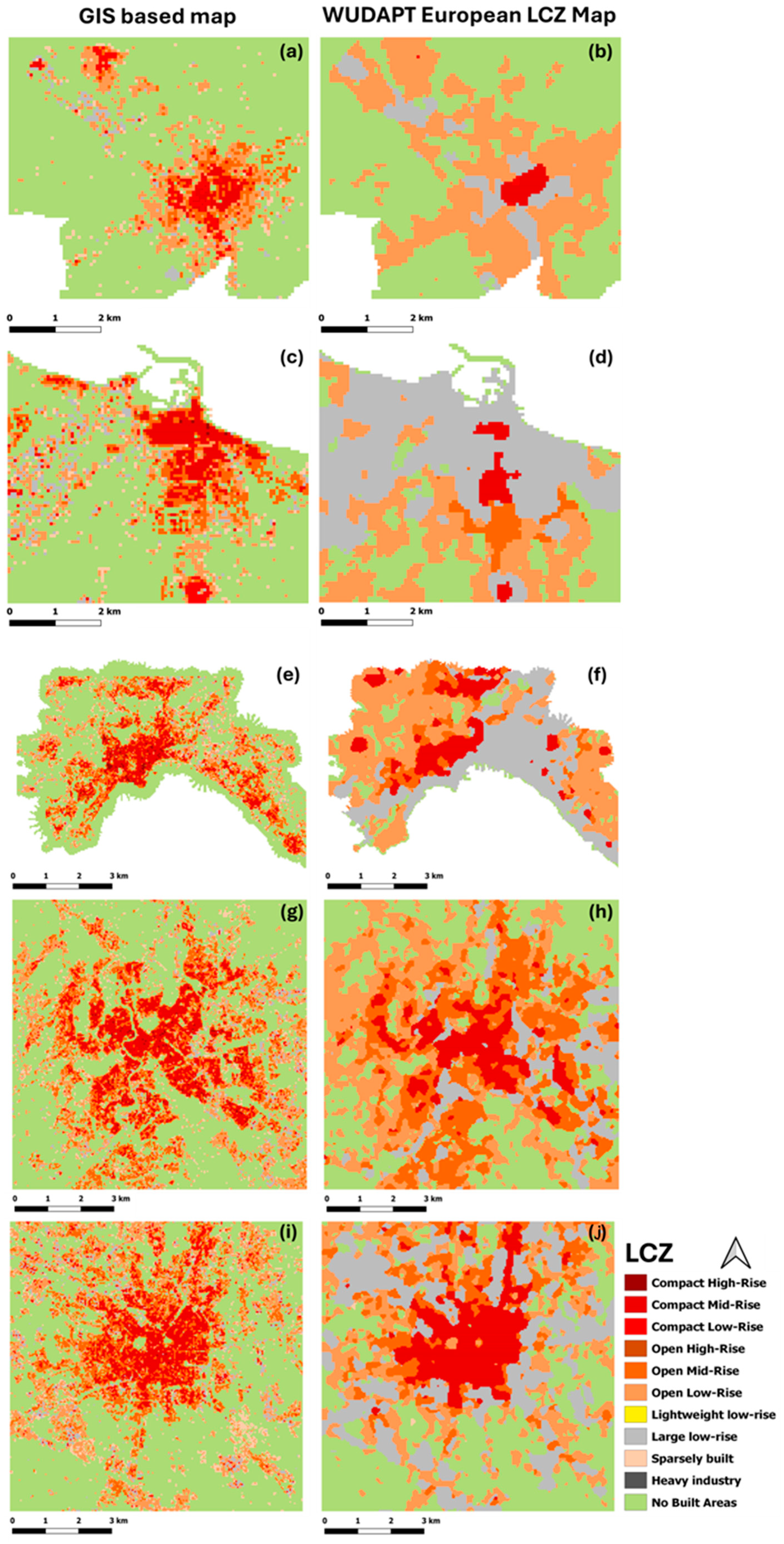Overall accuracy (OA) values were calculated by dividing the sum of correctly classified pixels (diagonal sum) by the total number of pixels, providing an overall percentage for classification accuracy [33]. The OA results revealed varying classification accuracy across cities: 73% for Lecce, 53% for Bari, 68% for Naples, 51% for Rome, and 48% for Milan. These values were obtained using a strict criterion that required exact pixel conformity to all UCPs tested, which might suggest that the actual percentage of correctly classified pixels might be higher in cases where tolerance or weighting adjustments were applied.

The OA values presented here are in line with the results of other studies, such as Hidalgo et al. [34], which also found discrepancies between the actual LCZ classifications and UCP value ranges. These deviations can be attributed to the inherent limitations of classifying LCZs based on predefined UCP thresholds, especially when morphologically and microclimatically similar LCZs are misclassified. In addition, the shape and size of spatial units in maps can affect the accuracy of classification. As noted by Wellinger et al. [35], LCZs typically do not conform to square shapes, resulting in mixed pixels along zone boundaries in gridded maps, which contributes to inconsistencies in UCP values.

Compared with the WUDAPT-based method, the GIS-based mapping approach offers greater accuracy and adaptability to local contexts. By utilizing high-resolution geospatial data from sources such as OpenStreetMap and digital elevation models (DEMs), along with complex morphological parameters like SVF and AR, GIS-based mapping provides a more detailed representation of LCZs. This is particularly advantageous in cities with intricate urban layouts, where WUDAPT, relying on satellite imagery and machine learning algorithms like Random Forest, struggles to capture vertical variability and distinguish heterogeneous urban forms [29,35]. Additionally, GIS methods allow for the adjustment of LCZ parameters based on city-specific characteristics, enhancing classification accuracy and relevance [35].

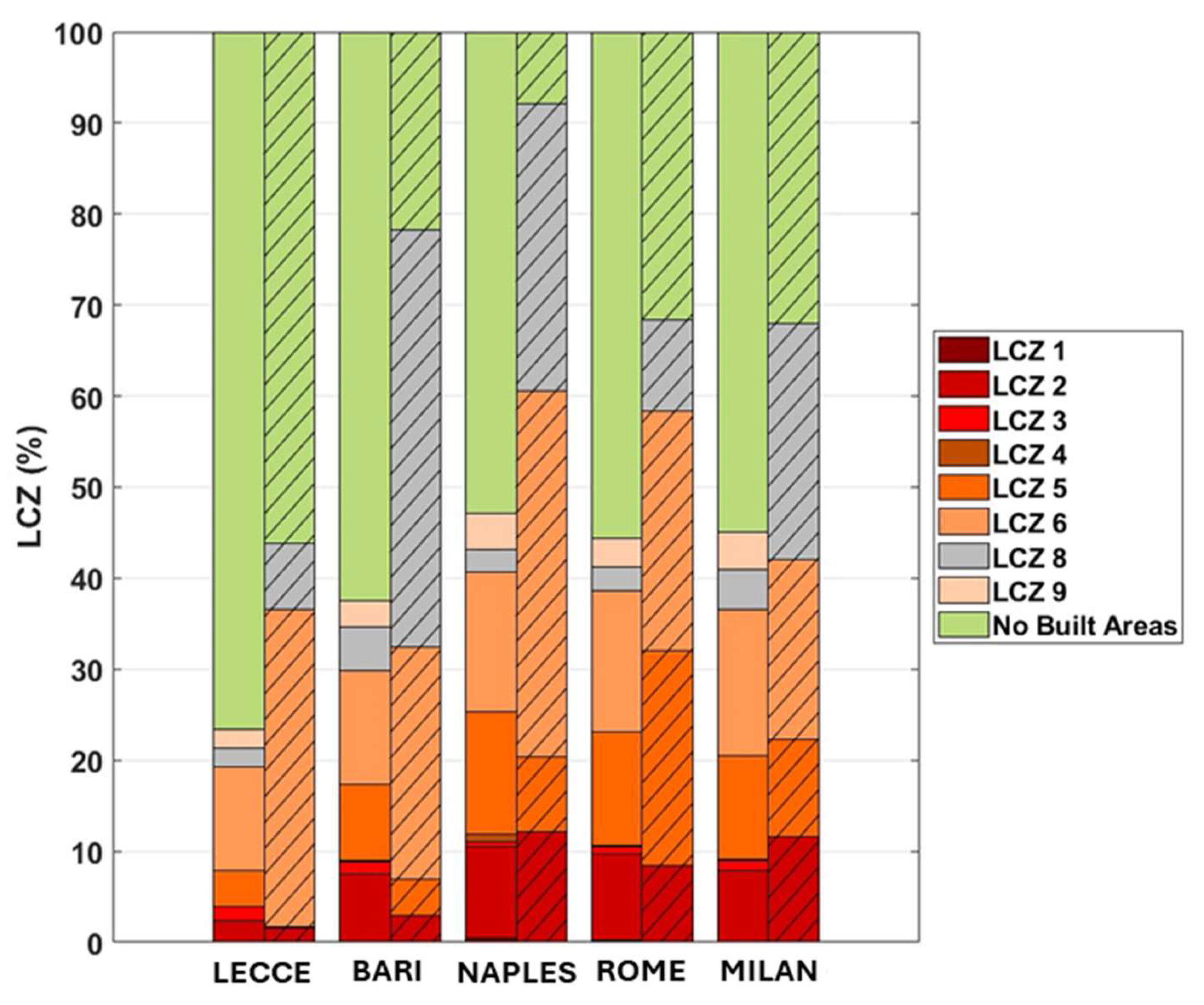
3.2. GIS-Based and WUDAPT European LCZ Map

In this section, the different distributions of LCZ classes from the two different maps were identified and quantified for all cities (Figure 4). The comparison of GIS and WUDAPT data shows significant discrepancies in the representation of LCZs in Italian cities (“No Built Areas” are not considered in the following analysis as it is idealized to make up for the lack of information of non-urban LCZs as explained in Section 2.4).

GIS data tend to present a more uniform distribution of LCZs, with a consistent presence of LCZ 2 (compact midrise), LCZ 5 (open midrise), and LCZ 6 (open low-rise) in all cities. For example, GIS data for Naples assign 10% to LCZ 2 and 13% to LCZ 5, while Rome similarly presents 9% for LCZ 2 and 12% for LCZ 5. In contrast, WUDAPT data show a more heterogeneous distribution, often attributing higher percentages to LCZ 6 (35% in Lecce and 40% in Naples) and LCZ 8 (46% in Bari and 32% in Naples).

Notably, LCZ 1 (compact high-density) and LCZ 4 (open high-density) are absent or minimally represented in both datasets, suggesting a low prevalence of these urban forms in the cities. LCZ 3 (compact low-density) also shows consistently low percentages, with GIS reporting a maximum of 2% in Lecce and WUDAPT recording almost negligible values in all cities. On the other hand, LCZ 9 (sparsely built-up industrial areas) shows strong differences, with GIS identifying significant contributions in Milan (4%), while WUDAPT reports values close to zero.

These discrepancies underscore the methodological differences in classification approaches between the GIS and WUDAPT datasets. GIS captures a finer granularity in urban morphology, while WUDAPT tends to emphasize broader classifications, with a focus on zones such as LCZ 6 and LCZ 8.

3.3. Diurnal Variability of LST in Different LCZs

This section compares the variability of LST across different LCZs, using both GIS and European LCZ map, for the cities of Lecce and Milan.

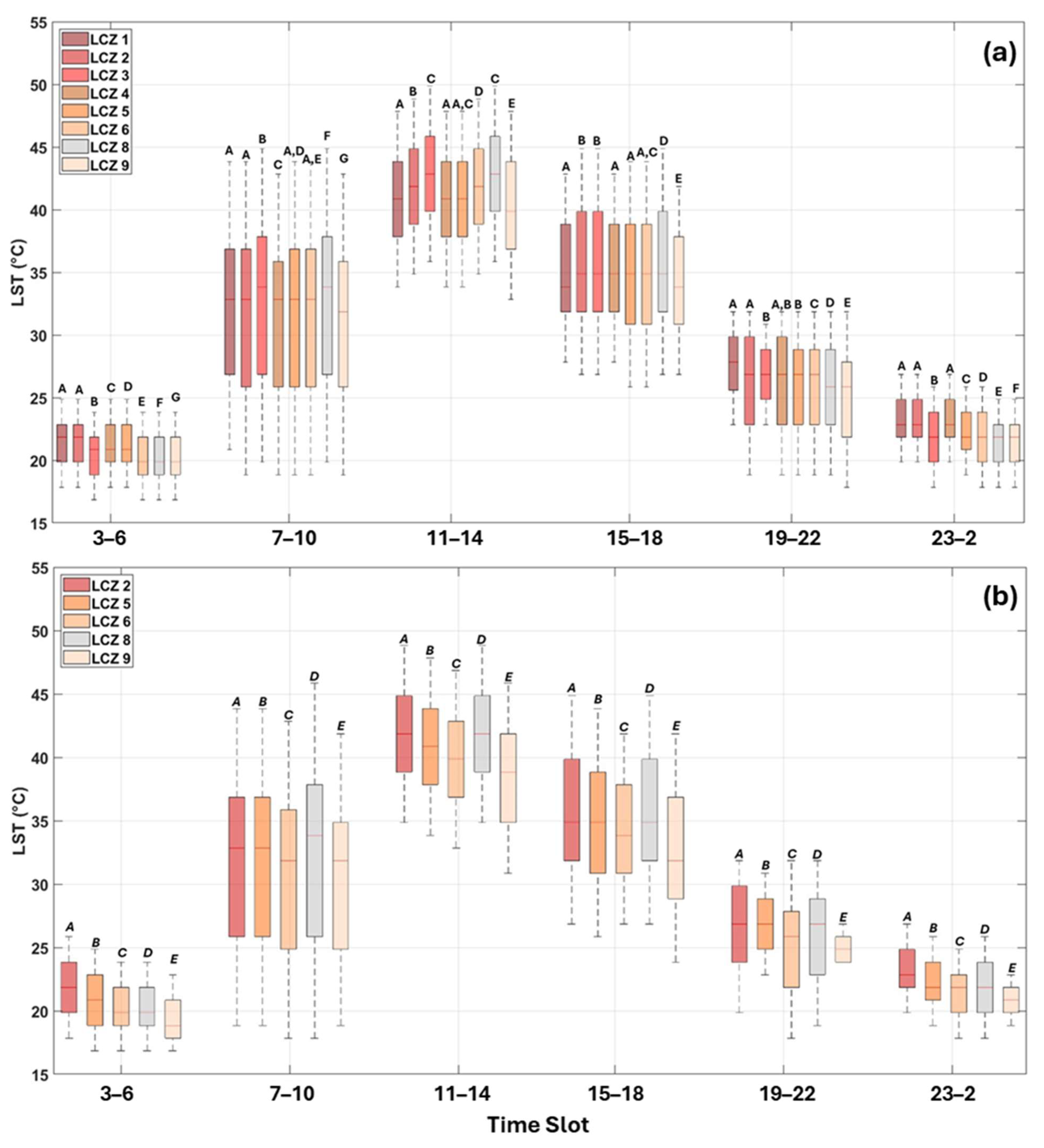
Statistical analysis with the nonparametric Kruskal–Wallis test identifies significant differences between the different LCZs, represented by the letters above each boxplot. The letters were assigned based on the p-values. Specifically, the first boxplot in each figure is always assigned the first letter of the sequence (i.e., “a/A”). Lowercase/uppercase characters are used to distinguish Lecce and Milan, respectively, while maintaining the same statistical significance. If the p-value for the second boxplot is less than 0.05, indicating a significant difference, it is assigned the next letter in the sequence. If the p-value is greater than 0.05, the second boxplot retains the same letter as the first, as no significant difference is detected. This method is applied throughout the entire sequence, ensuring a consistent assignment of letters based on statistical significance. In the case of mixed behavior (as in the case of Figure 5 for the WUDAPT European LCZ Map in Lecce), the box is assigned two letters, again based on the p-values. This letter assignment system clearly highlights the similarities and differences between the LCZs based on the statistical test performed.

3.3.1. Lecce

Figure 5a shows the diurnal cycle of LST for Lecce based on the GIS-based map, while Figure 5b presents the corresponding results using the WUDAPT map. Both figures show a characteristic diurnal trend, with the LST reaching its minimum values during the early morning hours and peaking between 11:00 and 14:00. There is a sharp rise in temperature in the morning, followed by a gradual decline in the afternoon and evening. These results validate the ability of ECOSTRESS satellite data to effectively capture the diurnal temperature cycle, accurately reflecting urban thermal dynamics.

Examining the differences between LCZs between 03:00 and 06:00, despite the general similarity of the median LST, specific patterns emerge. The classes of compact (LCZ2) and open (LCZ5) midrise have comparable LST values, as do the large low-rise (LCZ8) and sparsely built (LCZ9). However, significant differences are observed between the two low-rise building classes (LCZ3 and LCZ6), indicating that radiative cooling effects are more pronounced in these areas.

During the 07:00–11:00 period, substantial temperature differences emerge among all LCZs, underscoring the spatial heterogeneity of the urban thermal environment. This trend persists between 11:00 and 14:00, except for LCZ6 and LCZ9, which show no significant differences. LCZ2 records the lowest LST (43.6 °C), while LCZ8 reaches the highest value (45.8 °C), confirming that compact urban areas tend to experience slightly lower daytime peak temperatures than low-density areas. The urban core consistently records lower LST values than surrounding areas, a pattern consistent with Esposito et al. [14], who reported negative SUHI intensities in the Lecce core based on low-resolution satellite imagery. This urban cooling effect is particularly evident during the JJA season, probably due to reduced soil moisture in the suburban areas.

Between 15:00 and 18:00, the LST values of the compact (LCZ3) and large low-rise areas (LCZ8) converge (40.5 °C and 40.3 °C, respectively), while the low (LCZ5) and medium (LCZ6) open classes show similar temperatures (39.2 °C and 39.0 °C, respectively). During the evening transition (19:00 to 22:00), the two compacts midrise (LCZ2) and low-rise (LCZ3) areas follow comparable cooling rates, with average LSTs of 26.3 °C and 26.1 °C, respectively, while the other classes show more divergent thermal behaviors. This suggests that the compact zones experience prolonged heat retention due to accumulated energy during the day.

At night (23:00–02:00), LST distributions resemble those of the 03:00-06:00 period, albeit with slightly higher values, especially in denser urban areas. The highest LSTs are recorded in LCZ2 and LCZ3 (24.8 °C and 24.5 °C, respectively), while LCZ9 has the lowest values (23.2 °C).

Trend analysis of the WUDAPT-derived LSTs reveals similar temporal dynamics, except for the period 15:00–18:00, where LCZ6 aligns with LCZ3 instead of LCZ8. Throughout the day, statistical analysis confirms that the compact classes (LCZ2 and LCZ3) exhibit comparable LST trends, while the other LCZs show distinct thermal behaviors. During the 07:00-14:00 interval, compact areas maintain lower LSTs than openLCZs due to their higher heat storage capacity and increased shading due to dense building configurations. In contrast, nighttime conditions favor high LST in compact areas, as these areas release stored heat more gradually, potentially exacerbating nighttime overheating under certain environmental conditions. Overall, Figure 5a,b highlight the diurnal thermal response of different LCZs in Lecce, reinforcing the role of urban morphology in modulating LST dynamics. Compact urban areas generally have lower daytime temperature peaks but retain heat more efficiently at night, contributing to pronounced SUHI effects. The presence of vegetation further influences these patterns, with LCZ9 consistently showing lower temperatures due to evapotranspiration processes. In addition, coastal breezes from the Adriatic Sea likely enhance nighttime cooling, further modulating thermal contrasts between LCZs. These results underscore the complex interplay between urban structure, thermal properties, and microclimatic influences in shaping diurnal LST variations in Mediterranean cities.

3.3.2. Milan

Figure 6 shows the diurnal variation of LST in the different LCZs of Milan. The GIS-based map (Figure 6a) shows that during the early morning period (03:00–06:00), LCZ1 and LCZ2 have similar LST values, averaging about 21.00 °C. In contrast, LCZ9 records the lowest LST of 20.12 °C, highlighting the greater heat retention capacity of the compact urban areas (LCZ1 and LCZ2) compared to the stronger radiative cooling experienced in the less dense areas such as LCZ9. This difference can be attributed to the absence of high-rise buildings and narrow street canyons in LCZ9, which promote more efficient nighttime cooling.

During the morning period (07:00–10:00), LCZ1 and LCZ2 remain thermally similar, while LCZ3 and LCZ4 show distinct temperature trends. LCZ3 reaches the highest LST at 32.67 °C, followed closely by LCZ8 at 32.58 °C. LCZ9 remains the coolest, with an average temperature of 31.08 °C. In the midday hours (11:00 to 14:00), the disparities in LST between LCZs become more pronounced, with LCZ3 and LCZ8 recording the highest temperatures, with about 42.50 °C. In contrast, LCZ9 continues to record the lowest temperature, at 40.08 °C, underscoring the role of vegetated areas in mitigating temperature extremes during periods of peak warming. These results are in line with previous studies, which have shown that compact urban and industrial areas experience rapid temperature increases due to a high fraction of impervious surfaces [20,23].

The middle hours of the day present the greatest thermal heterogeneity, reflecting the different heating rates of different urban structures. In the afternoon period (15:00–18:00), LST values begin to decrease, although LCZ8 maintains the highest average temperature at 35.55 °C, while LCZ9 remains the coolest at 34.25 °C. As the evening progresses (19:00–22:00), LCZ1 and LCZ2 maintain high LST values, with recorded temperatures of 27.18 °C and 26.88 °C, respectively, while LCZ9 remains the coolest at 25.24 °C. Notably, a similar thermal pattern emerges between the compact and open LCZs, except for LCZ6 (open low-rise), suggesting that despite the variations in urban fabric, similar heat release occurs during this period.

During the nighttime period (23:00–02:00), differences in LST persist, with LCZ1 and LCZ2 having the highest temperatures (22.90 °C). This trend is very similar to that observed in the early morning hours (03:00–06:00), except for LCZ4, which shows a different cooling rate than the more compact zones. These observations are in line with literature findings indicating that denser LCZs retain heat more efficiently at night, while suburban and vegetated areas cool faster due to enhanced radiative cooling [17].

Figure 6b illustrates the distinct thermal behavior of LCZs, as captured by the European LCZ map, revealing pronounced temperature differences, particularly in the morning and midday hours. While the WUDAPT map effectively characterizes temperature variations among LCZs, the diurnal LST cycle shows substantial spatial heterogeneity. Overall, the most densely built-up classes (LCZ2 and LCZ5) show higher temperatures than the other LCZs, although these differences become less pronounced in the morning hours. LCZ8 consistently records high LST values during this period.

Comparative analysis of the results of the Kruskal–Wallis test between the GIS-based map and the European map of LCZs indicates variations in statistical differentiation and classification. The European LCZ map assigns greater variability to LCZs, suggesting greater statistical significance in LST distributions. This discrepancy is likely attributable to differences in classification methodologies and spatial resolution, which influence the statistical interpretation of temperature variations between LCZs.

Milan shows diurnal LST trends comparable to those observed in Lecce; however, the magnitude of the temperature variation between LCZs is more pronounced. Unlike Lecce, the composition of Milan’s land cover exacerbates temperature disparities, with the widespread use of concrete and asphalt—materials with high thermal inertia—contributing to prolonged heat retention, particularly in LCZ1 and LCZ3.

During the peak heating hours (11:00–14:00), the differences in LST become increasingly evident. The LCZ3 and LCZ8 reach the highest temperatures (42.50 °C), confirming that dense urban environments with minimal vegetation experience the most extreme warming. In contrast, LCZ9 remains cooler (40.08 °C), emphasizing the mitigating influence of green spaces during periods of intense solar radiation. These results are consistent with previous studies documenting rapid temperature escalation in urban environments due to extensive coverage of impervious surfaces [17,20].

In the afternoon cooling phase (15:00–18:00), LSTs decrease throughout the city, but differences between LCZs persist. LCZ8 maintains the highest mean temperature at 35.55 °C, while LCZ9 remains the coolest at 34.25 °C, highlighting the role of evapotranspiration in reducing heat retention. As the evening approaches (19:00–22:00), the compact urban LCZs (LCZ1 and LCZ2) continue to show high LSTs, indicative of prolonged heat accumulation and gradual nocturnal release by the impermeable surfaces. This trend extends into the early morning hours (03:00–06:00), where LCZ1 and LCZ2 show comparable LSTs, reinforcing their efficiency in retaining heat. Meanwhile, LCZ9, characterized by low-density development and substantial vegetation, experiences greater radiative cooling, resulting in lower temperatures in the absence of significant building structures.

3.3.3. Inter-City Comparison

Comparative analysis of the thermal responses of different Local Climate Zones (LCZs) in Lecce and Milan reveals distinct patterns, particularly in nighttime overheating. In Milan, denser LCZs (LCZ1, LCZ2, LCZ4, and LCZ5) experience higher nighttime temperatures, indicative of more pronounced urban heat retention. This trend contrasts with Lecce, where temperature variations among LCZs are less marked, except in the WUDAPT-generated map, probably due to the different distribution of LCZs. In Lecce, a well-defined temperature gradient is observed during the daytime period (07:00–14:00), with temperatures progressively increasing from denser to less dense LCZs. This pattern is less evident in Milan, where higher temperatures are primarily concentrated in high-rise areas (LCZ8 and LCZ3). The historic core of Lecce, mainly classified as LCZ2, maintains lower daytime temperatures due to the high albedo and thermal capacity of its historic buildings and paved roads, which limit heat peaks, consistent with findings in other Mediterranean cities [14,36]. In contrast, Milan’s larger size and higher urban density contribute to greater overheating, particularly during nighttime hours, intensifying the SUHI effect.

Despite sharing the same LCZ classifications, the thermal responses of corresponding LCZs differ between the two cities, underscoring the role of urban morphology, land cover composition, and climate in modulating LST variability. This aligns with findings from previous research in cities such as Valencia, Spain [23], and Xi’an, China [20], which highlight the influence of these factors on intra-LCZ temperature variations.

During the evening (19:00–22:00) and night (23:00–02:00) hours, both cities exhibit a progressive cooling trend, with urban LCZs retaining higher temperatures than suburban areas. However, this effect is more pronounced in Milan, likely due to its larger urban extent and higher building density in the high-midrise LCZs. The observed discrepancies between Milan and Lecce reinforce the importance of localized urban characteristics in shaping thermal responses, even within standardized LCZ classifications.

3.3.4. Contributions and Limitations

The findings contribute to a deeper understanding of SUHI dynamics in Mediterranean urban environments and emphasize the necessity of city-specific adaptation strategies to mitigate urban overheating effects. This research contributes to the broader understanding of urban climate adaptation by demonstrating the potential of high-resolution remote sensing for urban thermal assessments. The contributions gained can support data-driven policymaking and urban planning strategies aimed at mitigating the impacts of extreme heat in Mediterranean cities. The study also emphasizes the necessity of incorporating high-resolution thermal monitoring into climate adaptation policies, particularly in Mediterranean cities facing intensifying heat stress.

Despite the study’s contributions, several limitations must be acknowledged. While ECOSTRESS provides high-resolution thermal data, its irregular acquisition times limit temporal continuity, particularly during transitional periods such as early morning and late evening. Additionally, while the GIS-based approach offers improved classification accuracy, its scalability is constrained by the availability of high-resolution morphological data, limiting its applicability in regions with less detailed geospatial coverage. Furthermore, this study did not explicitly account for anthropogenic heat emissions, wind dynamics, and surface moisture, which are known to influence urban thermal behavior.

4. Conclusions

This study analyzed LST variability in Mediterranean cities using high-resolution ECOSTRESS data and two distinct LCZ classification methods: a GIS-based approach and the WUDAPT European LCZ map. This represents one of the first applications of ECOSTRESS data for diurnal thermal analysis in combination with LCZ classifications, offering a comprehensive assessment of urban heat dynamics during summer. The high spatial resolution and frequent temporal coverage of ECOSTRESS enable a more detailed analysis of urban thermal patterns compared to traditional in-situ measurements, which often lack representativeness in heterogeneous urban environments.

The primary objective was to evaluate classification accuracy and its impact on urban thermal analysis in Milan and Lecce. The GIS-based method, integrating high-resolution geospatial datasets, provided superior classification accuracy, particularly in cities with complex urban structures. In contrast, WUDAPT, which relies on satellite imagery and machine learning, exhibited broader classifications that sometimes misrepresented vertical variability, leading to lower accuracy in cities like Milan. The classification discrepancies between the two methods influenced the spatial distribution of LCZs: the GIS-based approach provided a more detailed representation, particularly for LCZ2, LCZ5, and LCZ6, whereas WUDAPT tended to overestimate LCZ6 and LCZ8. These differences directly affected the interpretation of LST patterns, with WUDAPT struggling to differentiate LCZs with similar urban morphologies.

The LST analysis revealed distinct thermal behaviors in Milan and Lecce, driven by differences in climate, urban form, and material properties. While LCZ classifications provided a useful framework for identifying thermal trends, results showed that identical LCZs can exhibit varying temperature responses depending on local conditions. This underscores the need to integrate LCZ classifications with localized climatic and morphological data for a more precise assessment of urban heat dynamics.

From a practical perspective, the findings offer important insights for urban heat mitigation strategies. The integration of high-resolution satellite data with detailed geospatial datasets allows for targeted identification of overheating zones, supporting climate adaptation planning. Urban policymakers can leverage this information to implement heat resilience strategies such as increasing vegetation cover, optimizing building materials, and enhancing urban ventilation.

Future research should consider additional variables related to the thermal properties of urban surfaces (e.g., roofs, walls, and roads) as well as meteorological forcings such as humidity, wind field, and anthropogenic heat fluxes to refine urban heat assessments. The greater spatial detail of remote sensing data should be enhanced by detailed land use mapping. Combining ECOSTRESS data within situ temperature measurements, reanalysis data (e.g., ERA5), and numerical modeling approaches would improve the robustness and generalizability of the results.