Construction and Application of Air Pollutants Emission Accounting Model for Typical Polluting Enterprises Based on Power Big Data

Abstract

Atmospheric pollution exacerbates climate change and ecosystem degradation. The accurate and timely calculation of emissions from various pollution sources is crucial for effective source control. This study is based on multi-source heterogeneous data from typical polluting industries, including electricity consumption, production load, and pollution emission data. It systematically analyzes multi-dimensional features and dynamic association mechanisms and constructs an Electricity–Production–Pollution recursive accounting model to quantify the response relationship between electricity consumption and pollutant emissions. The model establishes a theoretical framework and technical pathway for precise pollution source regulation driven by power big data. Using the emission accounting model, the annual PM_2.5 emission totals for cement, coking, brick, and ceramic industries in the pilot city were calculated. The relative error range compared to the urban emission inventory was −17.55% to 1.07%, and the emission calculation errors for individual companies were also within an ideal range (−19.31% to 15.63%). The model can perform real-time calculations of air pollutant emissions, such as daily emission changes, by monitoring an enterprise’s electricity consumption, thereby improving the precision of pollution source emission control.

1. Introduction

Globally, the rapid pace of industrialization and urbanization has led to increasingly severe air pollution issues, making it a critical challenge in environmental governance. Major pollutants, such as fine particulate matter (PM_2.5) and nitrogen oxides (NO_x), not only pose a serious threat to human health, but also further exacerbate climate change and ecosystem degradation. Against this backdrop, the accurate accounting of emissions from various sources is essential for the formulation of scientific and reasonable emission reduction policies and the optimization of air quality models.

Traditional air pollution emission accounting methods are mostly based on data declared by enterprises or rely on fixed emission factors for estimation, which have many problems, such as poor timeliness of data, low spatial and temporal resolution, and significant human errors. Traditional methods usually use provincial or municipal average emission factors, which are difficult for reflecting spatial heterogeneity. For example, the 2010 emission inventory of Guangdong Province showed that the NO_x emission density in the Pearl River Delta (PRD) region was four times higher than that in the western part of Guangdong, but the traditional accounting was unable to accurately locate the high-pollution grids (e.g., Dongguan and Foshan) [1]. A study of high-resolution emission inventories of anthropogenic sources of VOCs in Shaanxi Province also pointed out that the fixed emission factor method varies widely across regions and source types [2]. In the time dimension, fixed emission factors are mostly based on historical averages or laboratory measurements, which cannot adapt to technological advances and changes in fuel quality. Therefore, it is difficult to track short-term emission peaks and there is a lack of the ability to capture dynamic emission characteristics. For example, the study of SO₂ emission factor for thermal power plants in Guangdong Province shows that after the upgrade of desulfurization technology for coal-fired units, the actual emission factor is more than 30% lower than the default value of IPCC, but the traditional accounting still follows the old parameters, which leads to the overestimation of emissions [3]. In addition, the anthropogenic selection of activity level data directly affects the accounting results. Due to the lack of activity level data for solvent use sources, it is common to rely on empirical coefficients to estimate VOCs emissions, with uncertainties ranging from −25% to 42% [4]. The timeliness of the data declared by enterprises also directly affects the accuracy and timeliness of the accounting. As a result, it is difficult to meet the current requirements for dynamic supervision and refined management.

Electric power big data (EPBD) refers to massive, heterogeneous, and real-time datasets generated from power systems, including generation, transmission, distribution, consumption, and grid management processes. In recent years, EPBD, with its significant advantages of high spatial and temporal resolution, objectivity, and continuity, has brought brand new ideas and methods for environmental monitoring and pollution traceability. Studies at the provincial level in China have shown that there is a dual effect of electricity consumption as a secondary energy source on pollution. Such studies correlate provincial electricity consumption data with pollution indicators such as air quality index (AQI) and PM_2.5 by constructing regression models to provide a quantitative basis for policy formulation [5]. A study of the dynamic relationship between abrupt changes in electricity consumption patterns and air quality during COVID-19 verified the spatial shift of electricity consumption through high-resolution time-series data (e.g., daily electricity consumption and ground monitoring station data) on indirect effects on pollution, highlighting the need for data integration to incorporate sectoral categorization and geographic differences [6,7,8]. At the micro level, variables such as household electricity saving habits, income level and appliance ownership were included in the model to explain the heterogeneity of urban and rural electricity consumption and the difference in pollution contribution [9]. On the technology-driven side, the pollution assessment model under small samples is constructed by integrating electricity consumption, meteorological data, and pollution concentration at multiple monitoring points to improve the spatial coverage accuracy [10]. There exists a high degree of correlation between the production activities of industrial enterprises and their electricity consumption behaviors, especially the typical polluting enterprises with high energy consumption and high emissions, such as iron and steel, coking, cement, and other industries, whose electricity consumption data can indirectly reflect the dynamic correlation between the production intensity and the pollution emissions to a large extent. Through an in-depth mining of the coupling relationship between electricity big data and pollutant emissions, the construction of a data-driven emission accounting model is expected to break through the limitations of traditional accounting methods and realize real-time inversion and accurate assessment of emissions.

Taking typical polluting enterprises as the research object, this study proposes an air pollutant emission accounting model based on EPBD, which is dedicated to solving the deficiencies of existing accounting methods in terms of data timeliness, transparency, and traceability. By integrating the characteristics of electricity consumption, production process parameters, and environmental monitoring data of enterprises, we have systematically analyzed the characteristics of multi-dimensional data and the dynamic correlation mechanism. Combined with the machine learning modelling method, we constructed the Electricity–Production–Pollution (EPP) accounting model for typical polluting industries in the pilot city. It establishes a theoretical framework and technical path for the accurate supervision of pollution sources driven by electric power big data, and reveals the quantitative relationship between electric power consumption and pollutant emissions. The research results can achieve accurate the accounting and dynamic monitoring of emissions from typical polluting enterprises. It provides strong technical support for the tracking and control of air pollutant emission sources. It provides a solid scientific basis for enhancing the effectiveness of air pollution prevention and control, optimizing the means of environmental supervision and promoting energy saving and emission reduction in enterprises.

2. Current Research Status of Enterprise Pollution Supervision Based on EPBD

In today’s production and operational landscape, power energy has emerged as a cornerstone strategic resource and a critical production factor for businesses. Enterprise electricity consumption data serve as a precise reflection of economic activity and industrial operations, while EPBD holds significant potential for pollution monitoring across various industries. By constructing a pollutant emission accounting model based on EPBD, we can achieve rapid, accurate, and comprehensive monitoring, early warning, and control of industrial emissions, thereby providing robust support for environmental protection efforts.

2.1. Enterprise Pollution Monitoring and Prevention Based on EPBD

Yu Jin et al. [11] based on EPBD, constructed the enterprise pollution emission of abnormal electricity judgment model and enterprise stopping and reducing the production plan implementation monitoring model. Through the monitoring and early warning of pollution production, pollution control, and electricity consumption by enterprises, the rapid and accurate monitoring, early warning, and control of VOCs emissions can be realized. After on-site inspection, the model’s judgment accuracy rate was 100%. At present, the model has begun to deploy applications. It is of great significance in helping government departments quickly and accurately control VOCs emissions from enterprises and improve urban air quality. It can also eliminate the cost of purchasing VOCs online detection devices, which has great application prospects and broad market space. Hu Zhijun et al. [12] introduced EPBD to record the basic emissions of pollutants in the device by judging the detection threshold of pollution data; to realize the detection of VOCs pollution data by judging the detection limit value of pollution amount through the interval information of the warning segment; to establish a pollution propagation model by calculating the value of light source intensity and sunlight radiation intensity parameters to realize the quantitative analysis of pollution data; and to detect the different parameters through EPBD technology to realize integrated pollution prevention and control. The experimental results of the two studies show that the monthly emission of VOCs pollution within six months after the application of the method is reduced to less than 600,000 tons, and the prevention and control effect is obvious.

Relying on smart meters with existing hardware, Zhao L et al. [13] constructed an automatic monitoring system for polluting companies based on electric power data by combining the Internet of Things (IoT) technology, Convolutional Recurrent Neural Networks (CRNN) and Long Short-Term Memory Networks (LSTM). The system can automatically identify different types of equipment according to the load characteristics, and detect the illegal discharge behavior of enterprises in a timely manner by comparing and analyzing the operation of their pollutant production equipment and pollutant treatment equipment. Experimental validation shows that the overall identification mean square error of the model is only 0.5, and the accuracy of the model is higher than that of the RNN model and the LSTM model. The system can accurately and timely detect illegal behaviors and fill the loopholes in the supervision of enterprises by environmental regulators. Xi Zenghui et al. [14] obtained the enterprise air pollutant emissions based on the enterprise’s primary energy input and adopted smart meters to collect enterprise electricity consumption big data, combined with the results of enterprise pollutant emissions, to obtain enterprise pollution emission coefficients. Based on the enterprise pollution emission coefficients, the results of real-time total air pollutant emission measurement were obtained. This method can measure the total amount of air pollutant emissions from different industries using electricity data, which is convenient for providing the basis of environmental governance for the results of the total amount of air pollutant emissions, and is an important application of big data technology in the field of pollution prevention and control.

Ma Chunling et al. [15] proposed an enterprise short-term discharge monitoring and early warning method for power–environmental protection data fusion analysis. Based on high real-time power data, combined with environmental protection monitoring index data, supplemented by meteorological data and holiday data, the short-term emission prediction of each enterprise is realized through short-term power load data prediction. Chen et al. summarized the current research status of enterprise pollution emission modeling based on enterprise electricity consumption data, the identification and supervision of “scattered polluted” and “stealing and leaking” enterprises, the supervision and assessment of pollution emission during the special control period, as well as the construction of a refined emission inventory of air pollution sources at home and abroad [16]. The use of enterprise electricity consumption data can realize the accurate supervision of pollutant emissions from enterprises (especially small and micro enterprises).

However, most of the above studies only establish the quantitative relationship between EPBD and air pollutant emissions from the mathematical and theoretical point of view, but have not yet unearthed the potential physical relationship and logical correlation between the two, so that they cannot clarify the coupling principle and progressive relationship between EPBD and enterprise pollution monitoring and prevention. This is the fundamental problem that limits the scalability, interpretability, and regulatory scope of the model.

2.2. Enterprise Air Pollutant Emission Accounting Model

An algorithm study on electricity-based pollution accounting (EPA) was conducted in the field of enterprise pollutant emission accounting and forecasting. The research focuses on exploring the correlation between electricity data and pollution emissions, and is committed to constructing an accurate and efficient monitoring model, with a view to providing strong technical support for pollution control and environmental regulation. Various algorithms were used in this study. For example, the RBF neural network and BP neural network were used by Junhao Zhang et al. [17]; the former has a simple structure and strong learning ability, and the latter is good at dealing with nonlinear problems. Liu Zhonghui et al. [18] also used the BP neural network to identify equipment and determine the pollution emission status of the enterprise. LI G Y et al. [19] used the Apriori algorithm to analyze the correlation between electricity consumption and pollutant emissions, and combined it with the random forest (RF) algorithm to predict the emission concentrations; this has the advantages of high accuracy and fast training speed. Chi X et al. [20] explored the relationship between electricity data and air pollutant emissions in the foundry industry by building a cubic polynomial regression model. Zhao L et al. [13] combined the IoT technology, CRNN, and LSTMs to construct an automated monitoring system for polluting companies.

However, these algorithms have certain defects: RBF and BP neural networks may have problems of local extremes and slow training speed; the Apriori-RF algorithm has high computational complexity, which has an impact on the efficiency of big data processing; the CRNN and LSTM networks have complex structures and are prone to overfitting; and polynomial regression models are greatly affected by data distribution and outliers.

Consider that it is difficult for non-algorithmic researchers to address the inherent flaws of algorithms. Rather, it is the algorithm selection, model characterization, and data quality that can improve the final performance of the model. Therefore, consider choosing a more appropriate machine learning algorithm based on the logical needs of model construction.

2.3. Shortcomings of Current Studies

In summary, the enterprise pollutant emission accounting model based on EPBD still has the following deficiencies. Various model algorithms have different functional defects, which makes it difficult to meet the multiple needs of accounting; there are limitations in model adaptability, and the current pollution monitoring models may not be able to adapt to the pollution emission characteristics of different industries and enterprises; and some of the pollutant emission accounting models are overly complex, requiring a large amount of computational resources and data support, which makes it difficult to promote them in practical applications. It is evident that the emission accounting model requires further optimization. To expand the scope of the study and enhance the scalability of the model, it is necessary to increase the variety and number of modelling samples. To simulate and predict the emission situation in a more detailed way, it is essential to refine the data and information and model parameters to incorporate additional potential variables. Optimizing or innovating algorithms with higher computational power could improve the computational efficiency of the model and save computational costs. Finally, a comparative analysis of models in different industries should be strengthened to promote the application and development of pollutant emission accounting models.

We have already established an air pollutant accounting model for iron and steel enterprises based on electricity big data by refining the process-level electricity consumption and production data of iron and steel enterprises in our previous study, which initially elucidated the dynamic response relationship between electricity big data and pollution emissions, and to a certain extent improved the temporal refinement of emission accounting [21]. However, because China’s iron and steel industry is dominated by long-process iron and steel, the electricity consumption and pollution characteristics of different processes, such as coking, sintering/pelletizing, blast furnace ironmaking, and converter steelmaking, have large differences, and are affected by factors such as changes in the profits of iron and steel products and policies. The iron and steel industry is in a state of over-capacity, and usually iron and steel enterprises cannot produce at full design capacity, and therefore are not representative of other typical polluting industries. In addition, the study defaults to a linear relationship between the activity level of each process and the electricity consumption, and the accounting model thus constructed has some limitations.

Therefore, this study will take the cement, coking, brick, and ceramic industries as representatives, and study the construction, optimization, and application of the EPA model in other typical polluting industries, adjusting the methods and strategies of data collection, processing, analysis, and application, so as to make the logic of calculation closer to the actual production process, with a view to introducing more characteristic variables into the enterprise’s air pollutant emission accounting model. The purpose is to introduce more characteristic variables into the enterprise air pollutant emission accounting model, break through the constraints of a single industry, and enhance the scientific basis and interpretability of the model, so as to improve the accuracy of pollution emission accounting and the effect of emission dynamic monitoring.

3. Enterprise Air Pollutant Emission Accounting Model Construction

The process flow in the cement production, brick and tile production, coking industry, and ceramic products manufacturing industries is relatively short compared to that of the iron and steel industry, and the whole enterprise can be considered as a whole for this study in the process of constructing the model. It should be noted that the total power consumption in the production process of an enterprise, in addition to coming from purchased electricity, may also come from facilities such as the enterprise’s own power plant or waste heat power generation. As the electricity data used for modelling is purchased electricity data from the Electricity Big Data Centre, it does not include enterprise self-generation or waste heat generation. Enterprises that have confirmed the use of self-generated electricity or waste heat power generation through research are required to introduce an overall conversion factor based on the ratio of the total enterprise electricity consumption to the purchased electricity. In terms of model architecture, it mainly includes data collection and processing, feature extraction, and model prediction modules.

3.1. Data Acquisition and Processing

This study incorporates 2019 daily-scale electricity consumption data for each industry selected from the pilot city enterprise electricity data set, with enterprise Continuous Emission Monitoring System (CEMS) data obtained from the provincial ecological environment departments, as well as data from the pilot city air pollutant emission inventory and emergency emission reduction inventory. It also includes information on gross industrial output value, enterprise production capacity, enterprise energy consumption data, holidays, and data on the implementation of control measures. Because there are different types of data and different standards, the data need to be pre-processed.

Table 1. Basic information about variables.

Variable Name	Variable Type	Unit
Enterprise daily purchased electricity volume	Continuous input variables	Million KW·h
Corporate daily self-generated electricity output	Continuous input variables	Million KW·h
Industrial daily waste heat power generation capacity	Continuous input variables	Million KW·h
Corporate daily total electricity consumption	Continuous input variables	Million KW·h
Total industrial output value of enterprises	Fixed reference variables	10,000 yuan
Enterprise daily production capacity	Continuous reference variables	t
Enterprise annual production capacity	Continuous reference variables	t
Corporate annual energy consumption	Continuous reference variables	t (coal, oil, etc.)
Enterprise daily production load	Continuous output variables	%
Enterprise daily product output	Continuous output variables	t
Date	Continuous input variables
Holiday	Continuous reference variables	/
Weekday	Continuous reference variables	/
Pollution control measures	Continuous reference variables	/
Pollution control efficiency	Numeric variables	%
Pollutant emission factor	Numeric variables	kg/t
Enterprise pollution emissions (list)	Continuous output variables	t
Enterprise pollution monitoring (CEMS)	Continuous reference variables	t

is the list of the variables used and their statistical information. The fields of external data and internal data are unified according to the electric power basic code standard to avoid different coding forms for the same fields. The data types represented by data fields are maintained so that the fields correspond to the correct data types and avoid the phenomenon of storing numbers and times as strings. This is because there are differences in how different data types are called; secondly, it can improve the efficiency of data conversion when performing operations such as the aggregation of data; and thirdly, it is conducive to the screening of abnormal data and the discovery of abnormal data in advance. Null checking and format checking are performed on the data to form a standardized data format specification.

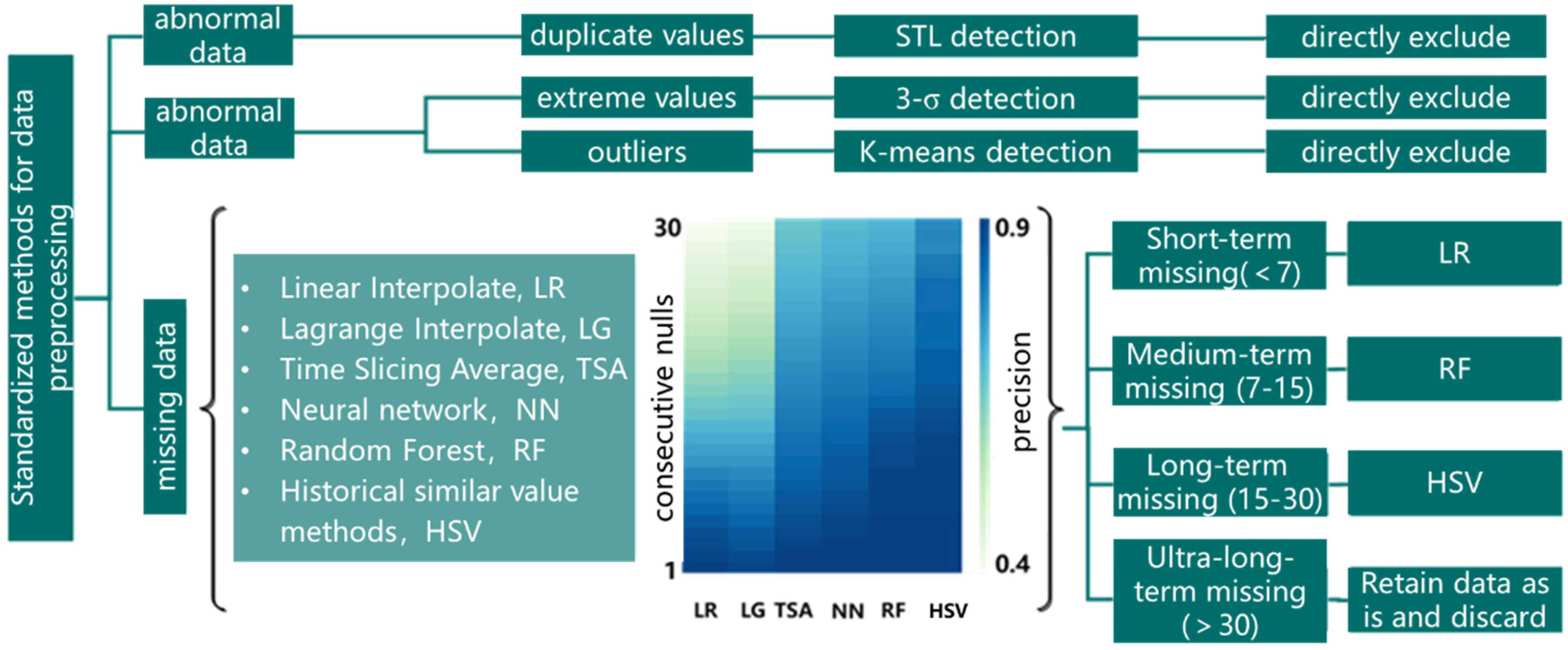
Through the application of statistical analysis, machine learning, and data mining methods, we explore the patterns, trends, and anomalies of data such as government public data, enterprise pollutant monitoring data, etc., study the governance algorithms of various types of data, realize the de-weighting, gap filling, and outlier processing of data, and standardize the data anomalies from the perspectives of qualitative and quantitative data. The method is shown in Figure 1. The 3-σ method, box-and-line diagram method, and K-means method, combined with the moving window method, are used to identify data outliers. The magnitude of data jumps is identified by moving the window, and if the magnitude of data jumps does not conform to the normal distribution, it represents an anomaly in the original data. The outliers can be effectively culled or corrected by empirical judgment. Duplicate tables in the dataset or duplicate data in the table are identified and eliminated by the STL tool. For missing values, it is necessary to categorize them based on the method of statistical analysis, use the combination strategy of multiple filling methods, and select the most suitable filling method according to the continuous length and characteristics of the missing data.

The number of consecutive nulls in the existing dataset ranges from 1 to 130. For short-term consecutive nulls (≤7 days), simple and efficient interpolation methods such as linear interpolation can be tried; for medium-term consecutive nulls (7 days < consecutive missing days ≤ 15 days), models such as limit gradient boosting algorithms are needed to achieve the filling; and for long-term nulls (15 days < consecutive missing days ≤ 30 days), the method of constructing the historical similarity values to fill them is tried. For consecutive missing days of more than 30 days, the original appearance is retained.

The historical similar value filling method constructed in this study is to use the data from similar days to supplement the missing data after extracting the recent one-year historical data. The steps are as follows. Construct the data set S′ = {A,B,C,D,E}, T = {T₁,T₂,T₃,…,T_n}, T ∈ A,B,C,D,E. Column A in the data set represents the original data, and column B is derived according to whether the data are missing, and column B is the missing label (0 means missing and 1 means is missing). It is assumed that there is a more similar periodicity of data fluctuations in the time period corresponding to consecutive missing data. The day labels are then calibrated based on the holiday, date, and weekday attributes. Column C contains the holiday labels (0 for holidays and 1 for being a weekday). Column D contains the date labels (1:31), and column E contains the weekday data (0:6). The values in column B are used to divide the S’ set of missing data and the S″ set of complete data. The single missing data f = {a_m, b_m, c_m, d_m, e_m} in S′ will be calculated separately from the complete data set S″ for similar days $d_i=\sqrt[2]{{\left(c_m-c_i\right)}^2+{\left(d_m-d_i\right)}^2+{\left(e_m-e_i\right)}^2}$. Arrange the d_i from largest to smallest to obtain d_j′. The selection of the number of similarity days has a more important impact on data completion; a single similarity day involves uncertainty, and too many similarity days will increase data uncertainty. Based on the 95% confidence interval test, this method sets the number of non-similar days to be 95% of the overall number of days. The similar day distance threshold d_limit = d_m′, where m is j × 95% rounded to the nearest whole number, dynamically selects N similar days with d_i < d_limit. At this time, to fill $a_m={\displaystyle \frac{\sum _1^N a_j}{N}}$, a_j is the day data corresponding to d_j. Repeat, moving data f to S″ until S′ is empty, completing the data fill as needed with the complete data set S″.

Through data optimization and cleaning, the daily scale EPP data of 27 cement enterprises, 4 coking enterprises, 10 brick enterprises, and 8 ceramics enterprises in the pilot city were obtained. Among the 27 cement enterprises, there are 23 grinding stations, accounting for 85% of the total number of cement enterprises. The 4 coking enterprises are all independent coking companies using mechanized coke ovens and ancillary equipment for coking. The brick and tile industry has various types of furnaces and due to different statistical caliber, the capacity unit is different, divided into 10,000 t/year, 10,000 pieces/year, and 10,000 m²/year. Ceramic industry product categories are different, and capacity units are also divided into 10,000 t/year and 10,000 pieces/year.

3.2. Model Building

The use of fossil energy affects, to a certain extent, the linear relationship between electricity consumption—production load—pollution emission. In order to further investigate the feasibility of the EPA model, it is necessary to first examine the correlation between industry emissions and electricity consumption. To facilitate the comparison between different industries, it is necessary to consider the consistency of data sources and the characteristics of industry emissions. In grinding station companies, SO₂, NO_x, CO, VOCs, and NH₃ emissions are rare, and there is a significant difference, so this study selected PM_2.5 and PM₁₀ as representative pollutants, and fitted the annual scale electricity consumption data to the particulate (PM_2.5 and PM₁₀) emission data in the 2019 pilot city emergency emission reduction inventory, followed by Pearson correlation analysis (see Equation (1)).

$$r={\displaystyle \frac{\sum _{i=1}^n\left(X_i-\bar{X}\right)\left(Y_i-\bar{Y}\right)}{\sqrt{\sum _{i=1}^n{\left(X_i-\bar{X}\right)}^2}\sqrt{\sum _{i=1}^n{\left(Y_i-\bar{Y}\right)}^2}}}$$

(1)

where $\bar{X}$ and $\bar{Y}$ are the sample means of variables X and Y, respectively.

The correlations between particulate matter emission and electricity consumption in the cement industry, coking industry, brick industry, and ceramic industry are calculated as 0.72, 0.97, 0.65, and 0.63, respectively. The correlation criteria are shown in

Table 2. Basis for determining Pearson’s correlation.

Correlation Coefficient	Degree of Correlation
0 < |r| < 0.3	weak correlation
0.3 < |r| < 0.7	correlation
0.7 < |r| < 1	strong correlation

, which shows that the electricity consumption and pollutant emissions for four typical polluting industries in the pilot city are strongly correlated, strongly correlated, correlated, and correlated. Therefore, it is feasible to use electricity consumption data to construct the pollutant emission model.

The sample size for correlation analysis is increased, and Pearson correlation analysis is performed between the daily scale electricity consumption data of enterprises in typical polluting industries in the pilot city and the daily scale emission data calculated based on CEMS, to investigate the feasibility of constructing the EPA model based on the EPBD and CEMS data. The results are shown in

Table 3. Correlation analysis results.

Industries	Electricity Consumption–Production Linear Correlation	Electricity Consumption–CEMS Linear Correlation
cement	strong correlation	correlation
coking	correlation	weak correlation
brick	correlation	weak correlation
ceramic	correlation	weak correlation

, with a weak correlation pattern. Further correlation analysis of the activity level (product output) data from the monthly statistical reports of enterprises in typical polluting industries with the monthly scale electricity consumption data, shows a correlation between the two, and it is significantly stronger than the correlation between electricity consumption and CEMS (Table 3).

The reason should be that the pollutant emissions of enterprises not only include the organized CEMS emissions, but also include the unorganized emissions and the organized emissions without CEMS installation. Constructing a relationship between electricity consumption data and CEMS data directly will leave out a portion of enterprise emissions and fail to characterize the true level of enterprise emissions. According to the previous analysis, it is clear that the pollutant emissions of the industry are strongly correlated with the electricity consumption data, so the electricity consumption–CEMS correlation analysis will show a weak correlation result.

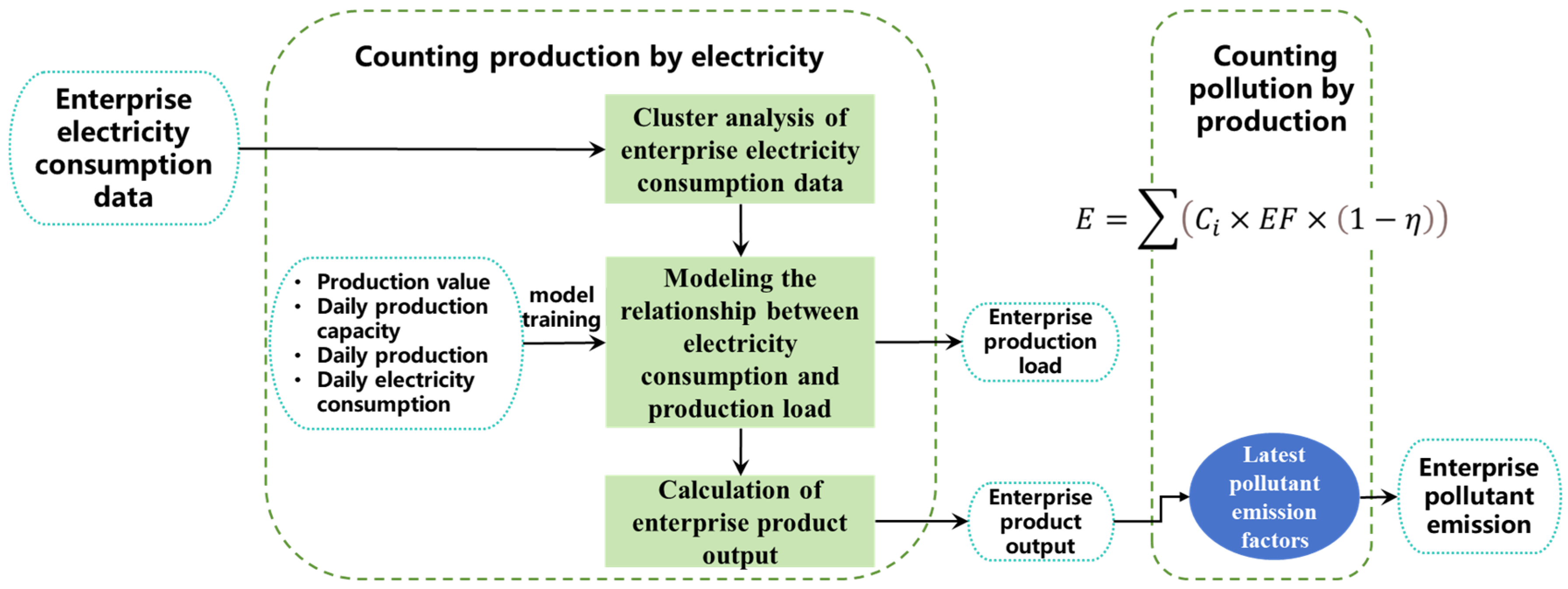
Therefore, in order to ensure the accuracy of data transmission and the comprehensiveness of the accounting link, the model first constructs the electricity–production (EP) relationship model based on the enterprise’s electricity consumption data and product output data, and then introduces the emission factor to accurately connect the production–pollution (PP) relationship. The EPP model of the enterprise is constructed according to the idea of “counting production by electricity and counting pollution by production”. The model architecture is shown in Figure 2. In the part of counting production by electricity, the production load of enterprises is more stable in different power zones. Based on clustering analysis, the electricity consumption data of different enterprises are graded to obtain the range of each electricity consumption zone. Subsequently, the production load analysis model is obtained by training the model with the eigenvalues of graded electricity consumption, industrial output value, enterprise production capacity, and daily scale production. Finally, the output is calculated based on the production load. In the part of calculating pollution by production, the daily scale air pollutant emissions of the enterprise are calculated based on the product output data and the latest pollutant emission factors.

3.3. Counting Production by Electricity

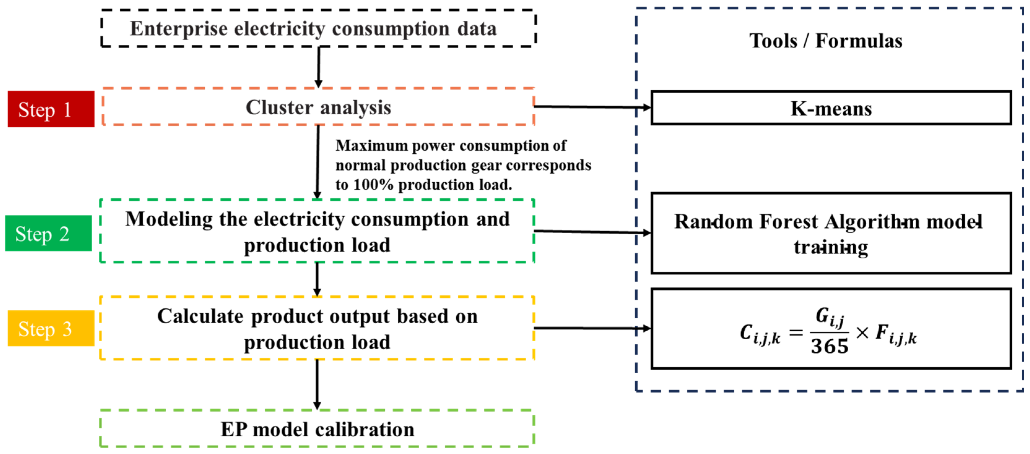
Counting production by electricity is the most important part of the enterprise EPP model, as shown in Figure 3, including three steps. Step 1 is the cluster analysis of enterprise electricity consumption data, using the Python 3.8.10 cluster analysis program to classify the day-by-day electricity consumption data of each enterprise. Step 2 constructs the relationship model between electricity consumption and production load. Step 3 calculates the enterprise product output, multiplying the process capacity and daily production load to derive the enterprise daily scale sub-process product output data.

The main purpose of constructing the relational model in Step 2 is to build a complex mathematical correspondence between the enterprise electricity consumption data and the production load data through machine learning algorithms. The random forest (RF) model captures complex nonlinear relationships in the data and is suitable for problems that are difficult to model with a linear model; it can effectively deal with large and high-dimensional data with high computational efficiency; it is robust to noisy data and outliers, and has high computational stability; it integrates multiple decision trees, which usually have higher prediction accuracy than a single decision tree; it is validated by out-of-bag (OOB) data, which reduces the risk of overfitting and improves the generalization ability of the model; and it provides feature importance indicators to help identify key features and facilitate feature selection and model interpretation. In view of these multiple advantages, this study utilizes the RF algorithm to train a production load forecasting model based on EPBD.

Step 1: Cluster analysis of enterprise electricity consumption data.

By mining the electricity consumption information of typical enterprises in different industries, this study finds that the electricity consumption of enterprises has obvious step-like characteristics. The actual production status of each enterprise can be roughly categorized into several kinds: in the stable production period, the production load is high, the power consumption is high, and the volatility of load and power is not large; in the control production period, the load level decreases, and the theoretical volatility of load and power is large, especially in some industries that contain processes that can be started and stopped at any time; and in the shutdown stage, the production load is low and the power consumption is low, and the load and power curves during the shutdown period show a smooth nature. There are also some special states, such as the cement industry, where there is an overloaded production state.

Due to the differences in the process and control measures of enterprises in various industries, it is not only a large amount of work but also a poor theoretical basis for the division of the state if the production state is divided for each enterprise individually. Therefore, according to the characteristics of each enterprise’s electricity consumption, the cluster analysis method is used to classify the electricity consumption, so as to characterize the different production states of enterprises every day.

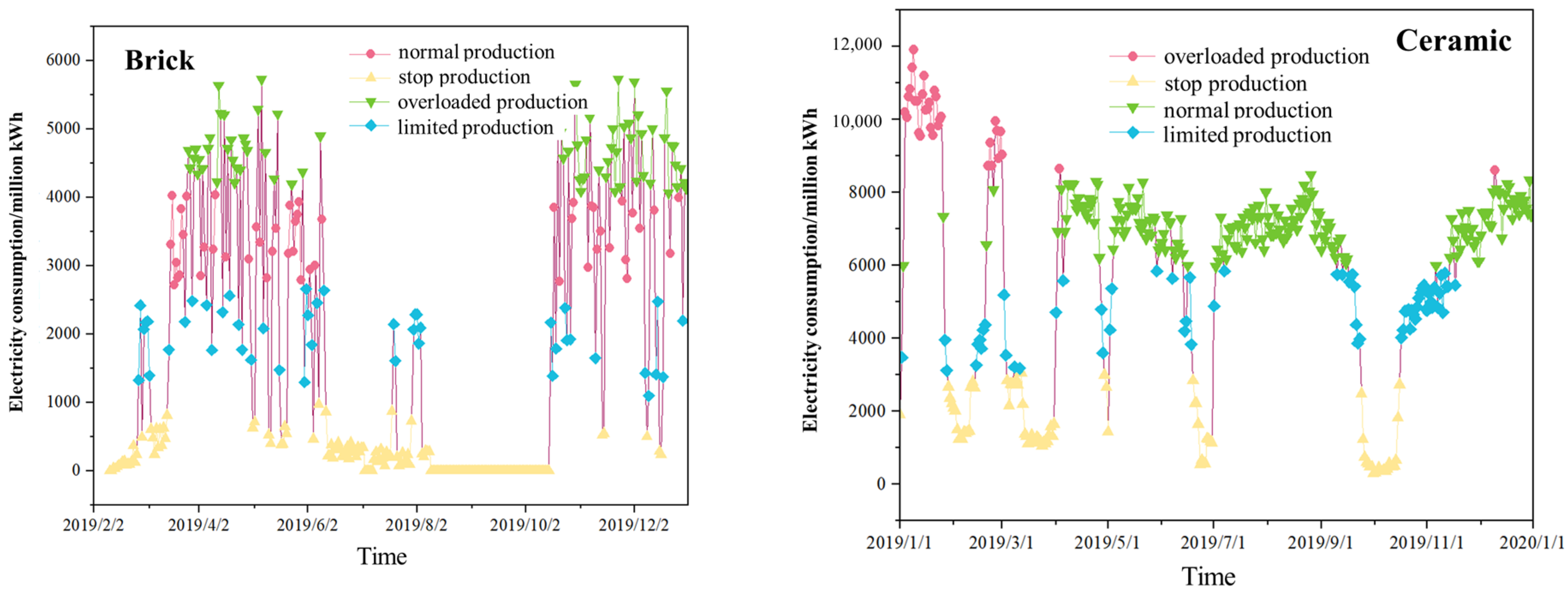
Specifically, the K-means algorithm, a python cluster analysis program in machine learning, is used to adaptively determine the number of power consumption clusters for each enterprise to differentiate between the different power consumption states of the enterprises. Based on the classification results, the electricity consumption of each industry can be categorized into four classes (Figure 4), i.e., normal production, production restriction, production stoppage, and overloaded production.

Step 2: Modeling the relationship between electricity consumption and production load.

Based on the capacity, production, and total industrial output values of different enterprises in the emergency emission reduction inventory, machine learning algorithms are used to clarify the specific functional relationship between electricity consumption and production load and to capture the nonlinear relationship and complex interaction effects among the data. A model is constructed of the relationship between electricity consumption and production load.

Due to statistical caliber and other reasons, there are differences in the capacity units based on the emergency emission reduction inventory. Therefore, this study establishes the load relationship model for different product units in typical industries separately. In the cement industry, the main pollutants come from clinker and powder mill, so the RF model of the cement industry only considers the clinker and powder mill enterprises in it, and the production capacity unit is 10,000 t/year. The brick and tile industries are classified into four levels according to the furnace type, and the production capacity units of different furnace types are different, so they are divided into 10,000 t/year, 10,000 pieces/year, and 10,000 m²/year for the establishment of the RF model, respectively.

The specific process of model construction is as follows. Obtain the day-by-day product output data of enterprises. When it is difficult to obtain day-scale data, the Litterman method from the field of econometric analysis can be considered [22]. High-frequency indicator information such as weekly data, holiday information, and information on the implementation of control measures are introduced as explanatory variables, and the low-frequency monthly-scale product output data are converted into high-frequency daily-scale data by estimating high-frequency interpolated series data. The daily production capacity of enterprises is taken as the daily average of annual or monthly production capacity. The ratio of daily production and daily capacity is then calculated to obtain the daily-scale production load data of the enterprise. The daily scale production load data and the clustered and graded daily electricity consumption data (with the graded logo) are taken as the main features, and the industrial output value, enterprise production capacity, enterprise energy consumption data, holiday information, and information on the implementation of control measures are taken as the other input features, which are inputted into the RF algorithm, to train the “Electricity Consumption—Production Load” model, namely EP model.

In this algorithm, 70% of the data is randomly used as the training set and 30% as the validation set. The RF algorithm in this study is based on the sklearn data package in scikit-learn (version 1.0. 1) and scipy (version 1.8.1). Due to the version issue, the output results need to be parameter corrected. The training set data is input into the above RF for continuous training. Each parameter is adjusted so that the forecasts calculated using the staggered power data of the validation set are constantly close to the true value of production loads.

The introduction of multiple other features and the high-frequency transformation of product yield data increases the uncertainty of the model’s prediction results while correcting the model accuracy and refining the time scale. Thus, the stability of the model was assessed by global sensitivity analysis, and the Sobol index method was used to quantify the contribution of each feature and its interaction to the model output.

Suppose the computational model is Y = f(X), where X = (X₁,X₂,…,X_n) is the input feature, Y is the output variable, and f is the model function. Each input feature Xi independently obeys its probability distribution P(X_i). Sample points are generated using random sampling or low-discrepancy sequences (e.g., Sobol sequences). Assume that N samples are generated, each containing n input features. For each sample point X^(j) = (X₁^(j),X₂^(j),…,X_n^(j)), calculate the output Y^(j) = f(X^(j)). The expected value E[Y] and variance D[Y] of the output variable Y are as follows:

$$E\left[Y\right]={\displaystyle \frac{1}{N}}\sum _{j=1}^N Y^{\left(j\right)}$$

(2)

$$D[Y]=E[Y^2]-(E[Y]{)}^2={\displaystyle \frac{1}{N}}\sum _{j=1}^N (Y^{\left(j\right)}{)}^2-(E[Y]{)}^2$$

(3)

The first order Sobol index $S_i$ measures the separate contribution of the input features${ X}_i$ to the output Y. The calculation starts by generating N auxiliary samples for each feature variable $X_i$, where $X_i$ varies independently from the other feature variables. The conditional expectation of Y at fixed ${ X}_i$ is $E\left[Y|X_i\right]$:

$$E\left[Y|X_i=x_i\right]={\displaystyle \frac{1}{N}}\sum _{j=1}^N{Y}^{(j)}{|}_{X_i=x_i}$$

(4)

The variance of conditional expectation $D\left[E\left[Y|X_i\right]\right]$ is as follows:

$$D\left[E\left[Y|X_i\right]\right]={\displaystyle \frac{1}{N}}\sum _{j=1}^N{\left(E\left[Y|X_i=x_i^{\left(j\right)}\right]-E\left[Y\right]\right)}^2$$

(5)

Then the index $S_i$ is as follows:

$$S_i={\displaystyle \frac{D\left[E\left[Y|X_i\right]\right]}{D\left[Y\right]}}$$

(6)

The second-order Sobol index $S_{i,j}$ measures the contribution of the interaction between the input variables $X_i$ and $X_j$ to the output Y. The calculation generates N auxiliary samples for each variable pair $\left(X_i,X_j\right)$, where$X_i$ and $X_j$vary independently from the other variables. Calculate the conditional expectation $E\left[Y|X_i,X_j\right]$ for Y when fixing${ X}_i$ and $X_j$:

$$E\left[Y|X_i=x_i, X_j=x_j\right]={\displaystyle \frac{1}{N}}\sum _{k=1}^N{Y}^{(k)}{|}_{X_i=x_i,X_j=x_j}$$

(7)

Calculate the variance of the conditional expectation $D\left[E\left[Y|X_i,X_j\right]\right]$:

$$D\left[E\left[Y|X_i,X_j\right]\right]={\displaystyle \frac{1}{N}}{\sum }_{k=1}^N{\left(E\left[Y|X_i=x_i^{\left(k\right)},X_j=x_j^{\left(k\right)}\right]-E\left[Y\right]\right)}^2$$

(8)

Then the second-order Sobol index $S_{i,j}$ is as follows:

$$S_{i,j}={\displaystyle \frac{D\left[E\left[Y|X_i,X_j\right]\right]-D\left[E\left[Y|X_i\right]\right]-D\left[E\left[Y|X_j\right]\right]}{D\left[Y\right]}}$$

(9)

The first-order Sobol index $S_i$ denotes the individual contribution of the variable ${ X}_i$. The second-order Sobol index $S_{i,j}$ denotes the interaction contribution of the variables${ X}_i$ and $X_j$. The sum of all Sobol indices should satisfy Equation (10) to verify the correctness of the calculation.

$$\sum _{i=1}^n{S}_i+\sum _{1\le i<j\le n}{S}_{i,j}+\cdots =1$$

(10)

Through the above steps, the contribution of each input variable and its interaction to the output is quantified, thus a global sensitivity analysis is performed.

Step 3: Calculation of enterprise product output.

Different enterprises in the cement industry contain different processes (single process for grinding or clinker only, or double process for both), and the different processes of an enterprise must be measured separately. The annual production capacity of the enterprise is evenly distributed to 365 days to obtain the theoretical value of daily production capacity; by multiplying the daily production capacity of each process with the corresponding date and the production load of the corresponding process, the measured value of its daily output can be obtained.

The product output for each process of an enterprise can be calculated by the following formula:

$$C_{i,j,k}={\displaystyle \frac{G_{i,j}}{365}}\times F_{i,j,k}$$

(11)

Style:

i, j, k represent firm, process, and date, respectively;

C represents real-time production accounting results (t);

G represents the annual capacity data of different processes of the enterprise (t);

F represents the production load (%).

3.4. Counting Pollution by Production

The correlation between the production load and electricity consumption of polluting enterprises is obvious, and real-time output can be obtained based on the calculation of production load, so this study uses the emission factor method to construct the pollutant emission accounting model of typical polluting industries. The production load data used in the accounting model come from the output of the relationship model between electricity consumption and production load of enterprises in various industries.

In addition, it should be noted that cement enterprises can be divided into grinding, clinker and dual-process categories according to the process, which need to be combined with the proportion of different processes for model construction. Dual-process enterprises are analyzed based on the literature [23,24] by folding the electricity consumption by clinker electricity consumption: grinding electricity consumption = 0.684211; other industries are considered by a single production line.

The formula for counting pollution by production is as follows:

$$E=\sum \left(C_{i,j,k}\times EF\times \left(1-\eta \right)\right)$$

(12)

E is the air pollutant emissions from the process of a company in a typical industry of air pollution, EF is the emission factor, C is the real-time production, η is the pollutant control and emission reduction efficiency, and i, j, and k represent the company, process, and date, respectively.

In particular, the installation of pollutant control measures in each enterprise was obtained from enterprise surveys and other environmental public reports. Pollution control efficiency η for each industry comes from the Manual for Preparation of Urban Air Pollutant Emission Inventory (

Table 4. Pollution control efficiency η for typical polluting industries (%).

Pollution Control Measures	SO2	NOx	VOCs	PM2.5	PM10	BC	OC
Flue gas circulating fluidized bed method	50	0	0	0	0	0	0
In-pile calcium injection method	50	0	0	0	0	0	0
Limestone/lime-gypsum method	80	0	0	57	75	57	57
Bisulfite method	80	0	0	57	75	57	57
Marine Law	80	0	0	57	75	57	57
Magnesium oxide method	80	0	0	57	75	57	57
Ammoxidation	80	0	0	57	75	57	57
Phase-locked coherent method	50	0	0	0	0	0	0
Rotary spray drying method	50	0	0	0	0	0	0
Other desulfurization technologies	40	0	0	0	0	0	0
Normal low nitrogen burner	0	22	0	0	0	0	0
High-efficiency low-nitrogen burner	0	42	0	0	0	0	0
Selective non-catalytic reduction method	0	30	0	0	0	0	0
Selective catalytic reduction method	0	42	0	0	0	0	0
Other denitrification technologies	0	20	0	0	0	0	0
Gravity settlement method	0	0	0	10	70	10	10
Inertia dust removal method	0	0	0	10	70	10	10
Wet dust removal method	20	0	0	50	90	50	50
Conventional electrostatic dust removal method	0	0	0	93	98	93	93
High-efficiency electrostatic dust removal method	0	0	0	96	99	96	96
Filtering dust removal method	0	0	0	99	99.5	99	99
Electrostatic baghouse dust removal method	0	0	0	96	99	96	96
Single-tube cyclone dust removal method	0	0	0	10	70	10	10
Multi-tube cyclone dust removal method	0	0	0	10	70	10	10
Unorganized dust general control technology	0	0	0	10	15	10	10
Unorganized dust efficient control technology	0	0	0	30	50	30	30
Other dust removal technologies	0	0	0	10	70	10	10

). The emission factor EF is the latest industry emission factor obtained by cumulative updating and expansion based on the nine technical guidelines for the compilation of pollution source inventories issued by the Ministry of Ecology and Environment, based on the results of the National Atmospheric Special Project and other research projects, and combined with the current production and pollution control processes, and the emission factors of key industries such as cement, coking, and iron and steel can be refined by the process. It is more comprehensive and detailed than the emission factors announced by the state, and is led by Tsinghua University and jointly researched by 7 universities and scientific research institutions, and released in the form of a group standard [25].

3.5. Validation of Model Results

3.5.1. EP Model Validation

The daily electricity consumption data are extracted from the calibration set, based on the established EP model, to forecast the production load of the enterprises. They are compared with the true value of production load corresponding to the electricity consumption data in the calibration set. The validation indicators are mainly standardized mean deviation NMB, absolute mean deviation NME, mean deviation MB, root mean square error RMSE, and the coefficient of determination R². The prediction results and errors of each industry are shown in Figure 5 and

Table 5. Validation indicators for EP models for typical polluting industries.

Parameters	NMB	NME	MB	RMSE	R2
Cement—10,000 t	1.514	14.021	0.517	6.477	0.972
Coking—10,000 t	0.959	10.569	0.372	5.602	0.975
Ceramics—10,000 pieces	−0.042	12.299	−0.016	6.373	0.970
Ceramics—10,000 t	−0.110	10.986	−0.047	6.829	0.971
Bricks—10,000 m2	−0.317	12.160	−0.140	7.275	0.966
Bricks—10,000 pieces	0.460	14.223	0.146	6.541	0.971
Bricks—10,000 t	0.530	13.745	0.186	6.463	0.973

. From the R², the fitting effect of the RF model is excellent; from the model validation results, the model can realize the enterprise production load forecasting based on electricity consumption data.

3.5.2. EPP Model Validation

Based on the established EPP model, this study calculates the 2019 air pollutant emissions of each industry and compares them with the 2019 urban inventory to verify the accuracy of the modeling results. Based on the EPP model, the total PM_2.5 emissions of the pilot city in 2019 are calculated as 2373.50 t in the cement industry, 194.43 t in the coking industry, 89.73 t in the brick industry, and 9.91 t in the ceramic industry, and the relative errors with the results of the urban inventory are −5.31%, −17.55%, −2.00%, and 1.07%, respectively. Among them, the coking industry results may be due to the small number of enterprises, the insufficient sample size available for the model of the relationship between electricity consumption and production load, and the larger error in the calculation of production load, thus leading to a larger error in the relevant emission accounting results.

In the cement industry, the clinker-cement dual-process enterprises allocate electricity to each process according to the clinker process/grinding process = 0.684211 after the introduction of the overall conversion factor for purchased electricity. The comparison of air pollutant emissions from three typical clinker-cement enterprises included in the EPP model with the urban inventory is shown in Figure 6. Comparing Figure 6A–C, the absolute errors of Enterprises A and C are both less than 1%, and the absolute error of Enterprise B is the largest, but still within 20%. From Figure 6D, the modeling error of cement dual-process enterprises mainly comes from the clinker process, due to the fact that the electricity consumption is concentrated in the grinding process, and the correlation between electricity and the grinding emissions is high. The clinker process needs to use a certain amount of fossil energy, resulting in a lower correlation between electricity and emissions. Overall, the air pollutant emission accounting model based on power big data can well account for the air pollutant emission level of cement enterprises.

Taking PM_2.5 as an example, the modeling results of air pollutant emissions from different enterprises in the coking, brick, and tile and ceramic industries and their error levels with the results of the urban inventory are all within the ideal range, as shown in Figure 7, with the relative errors ranging from −18.53% to 15.63%. Among 10 brick enterprises or 8 ceramic enterprises, only one enterprise has a large error, and the absolute errors of other enterprises are less than 5%.

In summary, the air pollutant emission accounting model based on EPBD can well portray the emission characteristics of air pollutants in the cement, coking, brick, and ceramic industries, and it can provide a reference basis for the accurate identification of emission sources and early heavy pollution warnings.

4. Model Application and Effectiveness Evaluation

Based on the EPP model constructed in the above study, the annual air pollutant emission characteristics of a dual-process cement enterprise (annual clinker production capacity of about 1.5 × 10⁶ t and annual grinding production capacity of about 1.8 × 10⁶ t) in the pilot city were analyzed for the year of 2019. By inputting the enterprise’s daily-scale purchased electricity data into the model, the enterprise’s air pollutant emission accounting is derived as shown in Figure 8. The annual emission accounting values of CO, SO₂, NO_x, TSP, PM₁₀, PM_2.5, BC, and OC are 32312.13 t, 2615.87 t, 26.02 t, 845.68 t, 469.26 t, 194.65 t, 1.76 t, and 2.85 t, which are similar to the relevant assessment results of the urban inventory, and the absolute error is within 1%.

In terms of pollution monitoring, the model can accurately capture the monthly change rule of the enterprise’s air pollutant emissions. From Figure 8, it can be seen that the enterprise’s air pollutant emissions in 2019 show obvious seasonal fluctuation characteristics, the emissions first decreased and then increased in the second quarter, and reached a peak in the fourth quarter. There is a high degree of consistency with the cement price fluctuation trend shown on the cement big data platform of the China Cement Network (https://data.ccement.com/, accessed on 1 January 2025), and the cement price fell first and then rose in 2019, with the rise mainly concentrated in the fourth quarter. In addition, it is obvious from the figure that the enterprise’s monthly emissions of various types of air pollutants have consistent fluctuation trends, so the fluctuation of a typical pollutant (e.g., PM_2.5) can be used to reflect the overall change rule of the enterprise’s air pollutant emissions. The model analysis shows that the pollutant emissions peaked in November and were at a lower level in April. Although emissions are lowest in February, the model selects April as the lowest-emission month to more accurately assess daily-scale emission differences, taking into account the factor of production days.

In terms of emission reduction management, the model demonstrates powerful analytical capabilities. By analyzing the daily emission data of PM_2.5 (Figure 9), the model is able to clearly identify changes in the production status of enterprises. It is found that the production activities of enterprises are significantly affected by the fluctuation of market cement prices, with production stopping or limiting in April, and normal or overloaded production in November. It can be inferred from the changes in the emission values in Figure 9 that if a company takes measures to stop production, it can reduce PM_2.5 emissions by about 0.8 t per day compared to the maximum production load condition. If the enterprise adopts production restriction measures, the daily PM_2.5 emissions can be reduced by about 50%. More importantly, the model can reflect the implementation effect of the emission reduction measures in real time, providing real-time monitoring tools for environmental regulators.

From Figure 10, the enterprise’s pollutant emissions mainly come from the clinker process, which is because the clinker production consumes more energy and uses more fossil fuels. The model’s identification of the main pollutant-emitting processes can provide a scientific basis for the enterprise to formulate accurate emission reduction strategies.

The practical application of the model demonstrates the following advantages: first, it is able to carry out high time-resolution pollutant emission accounting through power data, providing a reliable basis for the daily pollution monitoring of enterprises that have not installed CEMS; second, it can provide accurate emission reduction accounting for the emergency control of polluted days and the protection of major events.

5. Conclusions and Recommendations

This study constructs an air pollutant emission accounting model for polluting enterprises based on EPBD. By analyzing the heterogeneous data (electricity consumption, production load, and pollution emission indicators) from multiple sources of cement, coking, brick, and tile and ceramic industries in the pilot city, we systematically analyze the multidimensional features and dynamic correlation mechanism, and clarify the model structure of “electricity–production–pollution”, which is “counting production by electricity and counting pollution by production”. Based on the electricity–production coupling mechanism, machine learning algorithms are used to construct a high-precision mapping model of electricity consumption and production load. Combined with the real-time emission factor database, a production–emission transformation module is constructed to quantitatively characterize the daily scale pollutant emissions of enterprises. The research results can achieve accurate accounting and dynamic monitoring of emissions from typical polluting enterprises.

The model can accurately account for enterprise air pollutant emissions. Based on the emission accounting model, the total PM_2.5 emissions of the pilot city in 2019 were calculated as 2373.50 t in the cement industry, 194.43 t in the coking industry, 89.73 t in the masonry industry, and 9.91 t in the ceramic industry, and the relative errors with the urban emission inventory were −5.31%, −17.55%, −2.00%, and 1.07%, respectively. The error in comparing the emission accounting results of each enterprise with the existing urban emission inventory was within the desired range (−19.31% to 15.63%).

The model enables real-time, high-resolution enterprise emissions monitoring. Inputting the 2019 daily-scale purchased electricity data of a cement dual-process enterprise into the model can quickly account for the enterprise’s air pollutant emission results. By analyzing the daily PM_2.5 emission data, the model can clearly identify the characteristics of changes in the production status of the enterprise. When the emergency management of heavily polluted weather requires enterprises to take pollution reduction measures, the enterprise can reduce its daily PM_2.5 emissions by about 0.8 t by adopting shutdown measures, and the daily PM_2.5 emissions by about 50% by adopting production restriction measures. The model can complete real-time accounting of air pollutant emissions by monitoring the enterprise’s electricity consumption, improving the accuracy of the emission control of pollution sources. It helps enterprises to save energy and reduce emissions, and provides data support for policy making.

Despite the notable achievements and cross-industry generalization of the model achieved by this study, there are still some limitations that must be acknowledged. There are differences in the number and size of typical polluting enterprises between cities. The model does not introduce inter-regional differences as a modelling feature for the time being. The limited sample size in terms of spatial scale may also have a detrimental effect on the generalization of the model. The utilization of diverse data sources, accompanied by the varying statistical accuracy of each data type, necessitates the implementation of standardization governance and high-frequency data conversion, which in turn impacts data accuracy and, by extension, the reliability of the model. Future research should therefore explore the following aspects in depth: (1) expanding the sample size to cover more typical polluting enterprises in more regions to improve the universality of the model and (2) deepening the depth of cooperation between electric power big data and enterprises, establishing mutual trust in data, and obtaining more real values of the data through the integrated data sharing platform to alleviate the difficulty of data quality management and improve the accuracy of the data.

References

1. Pan, Y.Y.; Li, N.; Zheng, J.Y.; Yin, S.S.; Li, C.; Yang, J.; Zhong, L.J.; Chen, D.H.; Deng, S.X.; Wang, S.S. Study on Emission Inventory and Characteristics of Anthropogenic Air Pollutants in Guangdong Province. J. Environ. Sci. 2015, 35, 2655–2669. [Google Scholar] [CrossRef]
2. Lu, Q.Q.; Li, W.; Huang, G.Q. High-resolution and spatiotemporal distribution of VOCs anthropogenic sources in Shaanxi Province. J. Fujian Norm. Univ. (Nat. Sci. Ed.) 2018, 34, 32–43. [Google Scholar]
3. Dai, P.H. Establishment and uncertainty analysis of SO2 and NOx emission factors of thermal power plants based on CEMS data. Master Thesis, South China University of Technology, Guangzhou, China, 2016. [Google Scholar]
4. Bian, Y.H.; Fan, X.L.; Li, C.; Ye, X.; Wang, X.L.; Huang, Z.J.; Zheng, J.Y. Emission Inventory and Uncertainty of Non-road Mobile Machinery in Guangdong Province. J. Environ. Sci. 2018, 38, 2167–2178. [Google Scholar] [CrossRef]
5. Zhong, S.; Fang, Y.A.; Jing, H.J. Evaluation the impact of electricity consumption on China’s air pollution at the provincial level. PLoS ONE 2024, 19, 1537. [Google Scholar] [CrossRef]
6. Jang, M.; Jeong, H.C.; Kim, T.; Suh, D.H.; Joo, S.K. Empirical Analysis of the Impact of COVID-19 Social Distancing on Residential Electricity Consumption Based on Demographic Characteristics and Load Shape. Energies 2021, 14, 7523. [Google Scholar] [CrossRef]
7. Zheng, Y. Air pollution and post-COVID-19 work resumption: Evidence from China. Environ. Sci. Pollut. Res. 2022, 29, 17103–17116. [Google Scholar] [CrossRef]
8. Shanableh, A.; Al-Ruzouq, R.; Khalil, M.A.; Gibril, M.B.A.; Hamad, K.; Alhosani, M.; Stietiya, M.H.; Al Bardan, M.; Al Mansoori, S.; Hammouri, N.A. COVID-19 Lockdown and the Impact on Mobility, Air Quality, and Utility Consumption: A Case Study from Sharjah, United Arab Emirates. Sustainability 2022, 14, 1767. [Google Scholar] [CrossRef]
9. Li, Q.Y.; Yang, L.; Huang, S.; Liu, Y.Q.; Guo, C.Y. The Effects of Urban Sprawl on Electricity Consumption: Empirical Evidence from 283 Prefecture-Level Cities in China. Land 2023, 12, 1609. [Google Scholar] [CrossRef]
10. Chao, B.; Qiu, H.G. Air pollution concentration fuzzy evaluation based on evidence theory and the K-nearest neighbor algorithm. Front. Environ. Sci. 2024, 12, 1243962. [Google Scholar] [CrossRef]
11. Yu, J.; Yuan, H.H.; Wang, L.; Yan, D.; Xu, G.H.; Chen, C. Comprehensive Early Warning Control Analysis Method for Pollution Prevention and Control of VOCs Enterprises Based on Electric Power Big Data. Electr. Big Data 2022, 25, 71–75. [Google Scholar] [CrossRef]
12. Hu, Z.J.; Guo, Y.C.; Cheng, L. Research on the comprehensive prevention and control method of VOCs pollution supported by big data of electric power. Environ. Sci. Manag. 2024, 49, 97–101. [Google Scholar]
13. Zhao, L.; Wang, H.; Zhang, Z.Y.; Feng, S.M.; Gu, W.; Shi, X.X.; Miao, J.W. Enterprise Pollution Emission Monitoring System Based on Deep Learning of Power Data. In Proceedings of the 2022 International Conference on Automation, Robotics and Computer Engineering (ICARCE), Wuhan, China, 16–17 December 2022; pp. 1–5. [Google Scholar]
14. Xi, Z.H.; Wang, W.B.; Hong, Y.Q.; Yao, R.; Qu, Z.J. Study on real-time total emission measurement of air pollutants based on electric power big data. Environ. Sci. Manag. 2022, 47, 77–81. [Google Scholar]
15. Ma, C.L.; Wang, J.; Sun, C.X.; Chang, L. Power-environmental protection data fusion analysis for short-term enterprise emission monitoring and early warning. Electronic World. 2021, 15, 37–38. [Google Scholar] [CrossRef]
16. Chen, J.H.; Li, Z.; Liu, H.Q.; Gao, J.; Yang, Y.; Zhu, S. Progress of Research on Air Pollution Prevention and Control Based on Electricity Consumption Data of Enterprises. J. Environ. Eng. Technol. 2023, 13, 510–516. [Google Scholar]
17. Zhang, J.H.; Yang, X.L.; Han, X.M.; Ou Yang, L.; Liu, X.C. Comparison of the accuracy of enterprise pollutant emission intelligent measurement methods based on electric power big data. Ind. Heat. 2024, 53, 52–58. [Google Scholar]
18. Liu, Z.H.; Cai, G.Y.; Liang, B.J.; Luo, D.H.; He, J.F. Research on Pollutant Emission Monitoring Methods Based on Electricity Data Analysis. Inf. Technol. Netw. Secur. 2021, 40, 52–55+73. [Google Scholar] [CrossRef]
19. Li, G.Y.; Zhang, J.X.; Wen, X.; Xu, L.M.; Yuan, Y. Electric Power Consumption and Pollutant Emission: A Study Based on Big Data and Machine Learning Algorithm. In Proceedings of the 2022 34th Chinese Control and Decision Conference (CCDC), Hefei, China, 15–17 August 2022; pp. 200–205. [Google Scholar]
20. Chi, X.; Li, Z.; Liu, H.; Chen, J.; Gao, J. Predicting air pollutant emissions of the foundry industry: Based on the electricity big data. Sci. Total Environ. 2024, 917, 170323. [Google Scholar] [CrossRef]
21. Zhou, W.Q.; Yang, J.Q.; Ning, L.; Wu, H.C.; Bo, Y.; Zhang, Q.; Tian, H.Z. Construction and Application of Air Pollutant Emission Accounting Model for Iron and Steel Enterprises Based on Electricity Big Data. Environ. Sci. Res. 2024, 37, 299–307. [Google Scholar] [CrossRef]
22. Zhang, C.H.; Gao, T.M.; Chen, F. Research and application of frequency transformation method for economic time series. Stat. Res. 2017, 34, 92–100. [Google Scholar] [CrossRef]
23. Ghalandari, V.; Esmaeilpour, M.; Payvar, N.; Reza, M.T. A Case Study on Energy and Exergy Analyses for an Industrial-Scale Vertical Roller Mill Assisted Grinding in Cement Plant. Adv. Powder Technol. 2021, 32, 480–491. [Google Scholar] [CrossRef]
24. Ghalandari, V. A comprehensive study on energy and exergy analyses for an industrial-scale pyro-processing system in cement plant. Clean. Energy Syst. 2022, 3, 100030–100042. [Google Scholar] [CrossRef]
25. Chinese Society for Environmental Science. Technical Guidelines for the Preparation of an Inventory of Urban Air Pollution Sources: T/CSES 144-2024 [S]. 2024. Available online: https://www.ttbz.org.cn/StandardManage/Detail/108461/. (accessed on 1 February 2025).
Figure 1. Data preprocessing methods.
Atmosphere 16 00375 g001
Figure 2. EPP model architecture.
Atmosphere 16 00375 g002
Figure 3. Steps and methods of counting production by electricity.
Atmosphere 16 00375 g003
Figure 4. Examples of clustering and classification of enterprise’s electricity consumption.
Atmosphere 16 00375 g004aAtmosphere 16 00375 g004b
Figure 5. EP model validation for typical polluting industries. (AG) represent the prediction results of the cement, coking, ceramic, and bricks industries respectively. The abscissa represents the electricity consumption data of various industries (the calculation method of production load is different when the production units are different).The red dots indicate the prediction production load of the EP model. The blue bar chart represent actual production load.
Atmosphere 16 00375 g005
Figure 6. Results and error analysis of the EPP model for cement enterprises. (AC) represent the results of cement enterprises A, B and C respectively. (D) takes PM2.5 as the representative pollutant to compare and analyze the sub-process error results and total error results of the three cement enterprises.
Atmosphere 16 00375 g006
Figure 7. Results and error analysis of the EPP model for other industries. (AC) represent the results of coking enterprises, brick enterprises, and ceramic enterprises respectively.
Atmosphere 16 00375 g007
Figure 8. Monthly air pollutant emission accounting for a cement company.
Atmosphere 16 00375 g008
Figure 9. Daily air pollutant emission accounting from a cement company.
Atmosphere 16 00375 g009
Figure 10. Air pollutant emission accounting by process for a cement company.
Atmosphere 16 00375 g010