A Comparative Study on the Methods of Predictor Extraction from Global Sea Surface Temperature Fields for Statistical Climate Forecast System

Abstract

Statistical climate forecast systems typically do not use preceding global gridded sea surface temperature (SST) data directly; instead, they extract a single predictor (e.g., the Niño3.4 index) or multiple predictors (e.g., time series of several SST spatial modes). In this study, four different SST predictor extracting methods (one single-predictor method and three multiple-predictor methods) are comparatively analyzed within the same climate forecast platform incorporating either the linear regression (LR) model or the neural network (NN) forecast model. Rolling forecast experiments with the LR model show that, compared to a single strong SST predictor, only multiple predictors with more high-quality information (high signal-to-noise ratio) could improve the forecast skill. Sensitivity experiments also show that the influence of multiple-predictor extracting methods on forecast skill from the NN model is much weaker than that from the LR model. Moreover, whether or not multiple SST predictors are orthogonal might also affect the forecast skill. The above analyses provide a reference for establishing statistical climate forecast system based on preceding SST data.

1. Introduction

As a crucial component of the climate system, the ocean profoundly influences global climate through the exchange of heat, momentum, and matter with the atmosphere [1,2,3]. Meanwhile, the latest ocean state serves as a crucial foundation for short-term climate forecasts due to its large heat capacity and slower changes compared to atmospheric processes [4,5,6]. Particularly for a climate forecast with a lead time of more than three months, indicative signals mostly come from the ocean state [7,8,9]. Therefore, the sea surface temperature (SST), as a key variable representing ocean conditions, has been an essential input physical variable for statistical climate forecast systems [10,11,12].

Previous theoretical studies usually focus on the influence mechanism of a single SST variable (e.g., the Niño3.4 index) on climate forecasts [13,14,15]. A single SST variable (i.e., single predictor) is insufficient for a statistical climate forecast system to capture valuable indicative signals provided by global SST data [16,17]. Moreover, a statistical climate forecast system typically does not directly use all globally gridded SST variables [18,19]. One primary reason is the high correlation among the SST variables at adjacent grid points, which implies the presence of redundant information within the global gridded SST data. Additionally, if all the SST grid variables were employed as input predictors, the number of predictors (exceeding 1000) would be excessively high relative to the limited sample size of climate observations (less than 100), possibly giving rise to a severe overfitting issue. Consequently, it is of great significance for a statistical climate forecast system to extract a certain number of suitable predictors from the global SST data.

Although previous studies introduced many statistical forecast models with a few SST predictors [20,21,22,23,24,25], few focused on methods for extracting SST predictors. This study will compare four different extracting methods (one single-predictor method and three multiple-predictor methods) based on the same climate forecast system, which encompasses both linear and nonlinear regressions. Through comparative experiments, we endeavor to explore the following issues. Firstly, does the multiple-predictor lead to a notably enhanced forecast skill as compared to the single-predictor? Secondly, do different extracting methods exert a pronounced influence on forecast skill? Finally, are the aforementioned analyses dependent on the specific forecast model employed?

Here, we developed a forecast system for the June Western Pacific Subtropical High Ridge Line (WPSHRL) based on the preceding winter SST, using both the traditional linear regression (LR) model and the commonly used neural network (NN) model. Using this climate forecast system, the influence of the SST predictor extracting method was investigated. This paper is organized as follows: Section 2 presents the SST data and predictor extracting methods. Section 3 introduces the forecast system and related techniques. Section 4 illustrates the comparison among these different extracting methods. Finally, Section 5 presents the discussion and Section 6 provides the conclusions of the paper.

2. Data and Preprocessing

2.1. Data and Preliminary Analyses

The monthly SST data from 1961 to 2022 were downloaded from the Physical Sciences Laboratory [26]. In this study, only the winter SST anomaly, encompassing December of the previous year, January, and February, was used to extract predictors. The June WPSHRL data, representing the mean latitude position of the isoline where 500 hPa zonal wind u = 0 and ∂u/∂y > 0 surrounded by the 588 dagpm contour [27], were obtained from the National Climate Center of China. Due to the unavailability of data after 2016, the June WPSHRL data for recent years were manually calculated based on ERA5 reanalysis data, following the same definition.

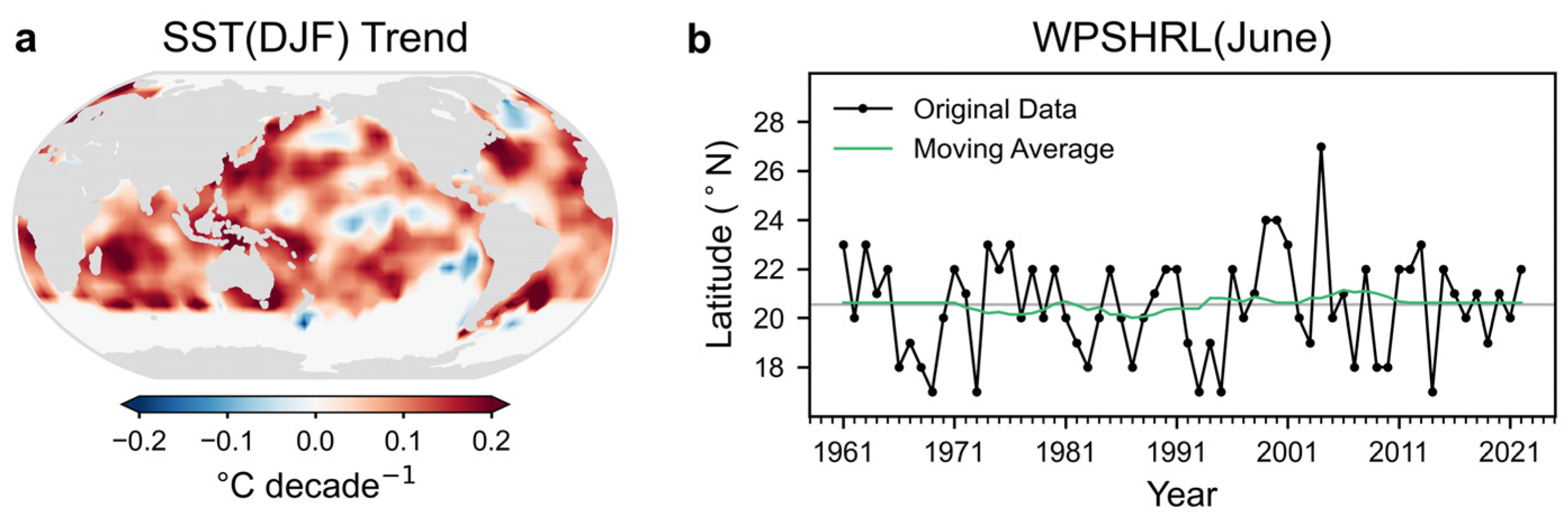
The winter SST displays notable decadal trends associated with global warming, whereas the June WPSHRL does not exhibit such trends (Figure 1). Before incorporating these variables into the forecast system, both the winter SST anomalies and the June WPSHRL were detrended using a 21-point moving average. Additionally, the detrended June WPSHRL data were normalized to the range of −1 to 1 (i.e., June WPSHRL index, hereafter referred to as WPSHRL). Based on the ranking of the WPSHRL from 1961 to 2022, the lowest and highest ~1/4 of years were identified as anomaly events. Among these 31 anomaly events, 16 were classified as low-WPSHRL years and 15 as high-WPSHRL years.

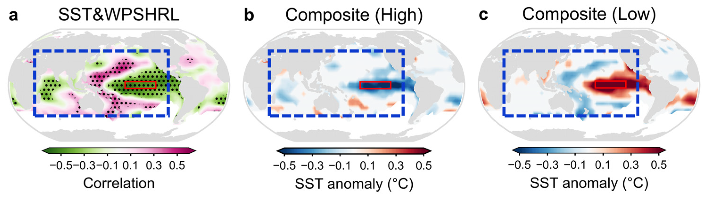
To better understand the design concept underlying SST predictor extracting methods, an analysis is first conducted on the correlations between the detrended preceding winter SST anomalies (hereafter referred to as SST) and WPSHRL (Figure 2). Consistent with previous studies, the Niño3.4 region (red-boxed area in Figure 2) provides the strongest indicative signal [28,29,30,31,32], and the linear correlation coefficients between SST and WPSHRL can reach −0.48. This is the reason the single-predictor method chooses the Niño3.4 index as the predictor. Furthermore, it is noteworthy that the SST indicative signals are predominantly located in the Pacific and Indian oceans (blue-boxed area in Figure 2). Consequently, one multiple-predictor method extracts SST predictors from these regions instead of from the entire global oceans.

2.2. SST Predictor Extracting Methods

There might be many approaches to extracting multiple SST predictors. In this study, we only explore two common and feasible ones: the ZONE approach and the EOF approach. Similar to the representative station [33,34,35], the ZONE approach selects 20 representative regions from the global SST field. The specific procedure is as follows: First, the SST grid with the largest year-to-year fluctuation is selected as the representative grid. Next, this representative grid and surrounding highly correlated grids (correlation > 0.6) are clustered together to form a single zone. Subsequently, this demarcated zone is taken out from the global SST field. This process is repeated until a total of 20 representative zones are established. The average SST of each zone serves as the candidate predictors. Principal component analysis, also known as empirical orthogonal function (EOF) analysis, is a commonly used tool in climate studies [36,37,38]. Here, the EOF analysis is used to select SST predictors (i.e., EOF approach). The time series of 20 leading EOF spatial modes (i.e., EOF principal components) serve as candidate predictors. The predictors derived from the EOF approach are sourced from two different SST spatial areas: the entire global oceans (EOFg) and the preliminarily selected regions (blue-boxed area in Figure 2, EOFp). For convenience in comparison and reference, the four SST predictor extracting methods used in this study are listed in

Table 1. Four SST predictor extracting methods.

Name	Number of Predictors	Extracting Approach	SST Spatial Area
Niño3.4	single	Niño3.4 index	Niño3.4 region
ZONE	multiple	representative zone	global oceans
EOFg	multiple	EOF	global oceans
EOFp	multiple	EOF	Pacific and Indian oceans

.

Figure 3 illustrates the 20 zones selected by the ZONE method, along with the corresponding SST time series. To clearly display the SST time series, only six representative zones that have the best correlation with WPSHRL are demonstrated. Because the ZONE approach prioritizes selecting the zone with the strongest SST fluctuation first, the ZONE number reflects the intensity of SST fluctuation. Consequently, the time series of ZONE1 and ZONE2 show relatively stronger amplitudes than the other zones. ZONE1 and ZONE2 are local in the central-eastern equatorial Pacific and typically exhibit consistent signs of fluctuation. In addition, ZONE1 and ZONE2 have strong correlations with WPSHRL (−0.48 and −0.54), while ZONE7, ZONE9, ZONE11, and ZONE18 also show relatively strong correlations (an absolute value more than 0.25). Because ZONE7, ZONE9, ZONE11, and ZONE18 are located far apart, their time series differ obviously from each other.

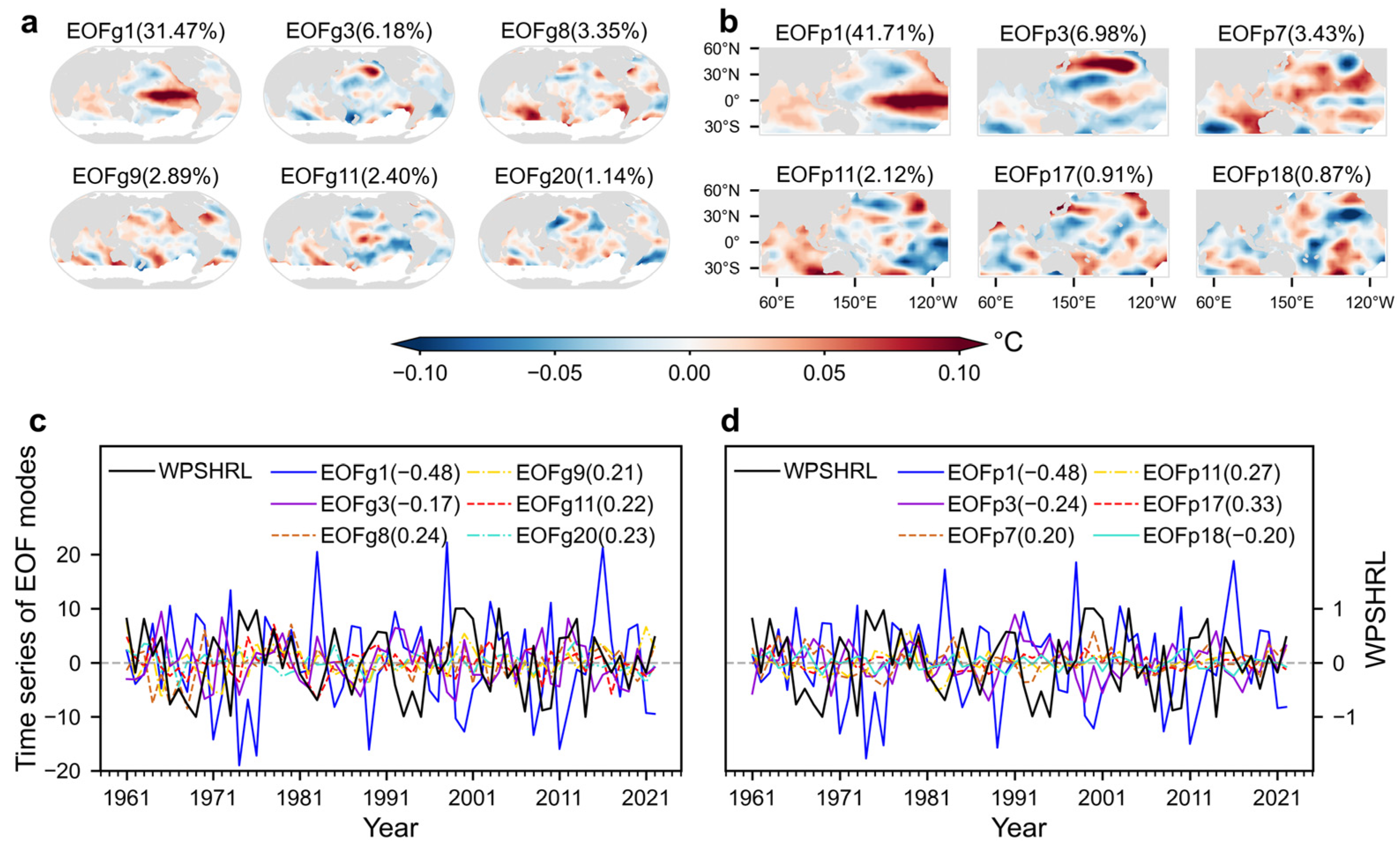
Figure 4 illustrates the SST predictors extracted by the EOF approach. Regarding the global SST field (i.e., EOFg), the leading 20 EOF modes can explain 87.55% of the original SST field. Focusing on the area of the Pacific and Indian oceans (i.e., EOFp), the leading 20 EOF modes can explain 93.02% of the original field. Here, only the six EOF modes that have the best correlation with WPSHRL are shown. The first and third EOF modes from the EOFp method (i.e., EOFp1 and EOFp3) are generally consistent with those from the EOFg method (i.e., EOFg1 and EOFg3). Compared to EOFg1 (31.47%) and EOFg3 (6.18%), EOFp1 (41.71%) and EOFp3 (6.98%) contribute more to the original SST field. The linear correlation between EOFp3 and WPSHRL (−0.24) is slightly stronger than that of EOFg3 (−0.17). Taken overall, the time series of EOFp modes exhibit slightly stronger correlations with WPSHRL than that of EOFg modes. This can be explained by the fact that the preliminarily selected SST regions (i.e., Pacific and Indian oceans) used in the EOFp method exclude those SST regions lacking obvious indicative signals. Finally, it is important to note that the EOF modes and their corresponding time series are mutually orthogonal. This differs from the ZONE approach.

3. Forecast System and Estimating Method

The influence of SST predictor extracting methods on forecast skill may depend on the specific forecast model employed. To test this, two different regression models are employed in our forecast system: linear regression (LR) and neural network (NN). Given the potential for overfitting due to small sample sizes, forecast skill is estimated using rolling forecast experiments. Additionally, the forecast skill for anomaly events is also analyzed, as climate forecasts focus more on such events.

3.1. Forecast System

The climate forecast system developed by this study is a framework (i.e., the model parameters to be determined) that incorporates either LR or NN. Prior to conducting forecasts, these undetermined parameters (excluding hyperparameters) are established based on all available samples (i.e., samples before the predicted year). In other words, the relationship between SST and WPSHRL in the forecast system is continuously updated due to newly added samples from the latest year.

When using multiple-predictor methods, it is necessary to consider selecting a set of optimal predictors from the 20 SST variables. In the LR framework, this problem is solved by the stepwise regression method. Only predictors with a significant improvement on the predictand (i.e., WPSHRL) are retained while minimizing the number of predictors as much as possible to reduce the possibility of overfitting [39,40]. The technical details of stepwise regression can be found in the statistical textbooks [41,42].

The fundamental theory of the NN model can be found in the textbook about machine learning [43]. Here, we focus on illustrating how to use the NN model. Considering the limitation of sample size, the number of NN model parameters (i.e., the weights and biases associated with each layer) cannot be too large. Therefore, a shallow NN model with one hidden layer is chosen. There are two architecture hyperparameters for this NN framework: the number of input variables (Nin) and the number of neurons in the hidden layer (Nhid). The first Nin (Nin ≤ 20) SST variables that have the best correlation with WPSHRL are chosen as input predictors. Unlike the LR framework, which can calculate how many SST predictors (similar to Nin) are optimal for establishing a forecast model, the architecture hyperparameters for the NN framework (i.e., Nin and Nhid) need to be preset based on previous experience. We tested several architectures of the NN framework (hereafter Nin-Nhid), such as 4-2, 4-3, 6-2, 6-4, 8-4, 8-6, 10-4, 10-6, 12-4, and 12-6. The experiment results indicate that once Nin exceeds 6, there is no substantial enhancement in the forecast skill. Meanwhile, the influence of Nhid on the forecast skill is negligible. Therefore, the NN architecture is set to 6-4 for all the experiments shown in this study. It is noteworthy that, under the condition of small sample sizes, the performance of the NN model is unstable and sensitive to the random seeds for initialization [44]. Thus, using some techniques [24,45], this NN framework first selects 10 good seeds from 200 random seeds. Then, 10 NN models can be trained with these 10 good seeds, and the final output predictand is the average of the 10 corresponding predictands (i.e., ensemble mean). The stability of forecast results with the NN framework is shown in Figure A1.

3.2. Estimating Method

The rolling forecast technique is often used to estimate the forecast system [46,47,48]. Considering the limitation of sample years (1961 to 2022), the rolling forecast experiment used in this study consists of two parts: forward rolling forecast experiment (from 1992 to 2022) and backward rolling forecast experiment (from 1991 to 1961). In the forward rolling forecast experiment (i.e., the commonly used rolling forecast), all available samples (from 1961 to the year before the predicted year) are used for the establishing forecast model. As for the backward rolling forecast experiment, the order of sample years is assumed to be reversed (from 2022 to the predicted year). To summarize, all sample years can be predicted by the rolling forecast experiment.

Forecast skill is usually quantified by the linear correlation coefficient (Cor) between observations and forecasts [49,50,51,52]. In this study, the probability of detection (POD) and false alarm rate (FAR) for anomaly events are also analyzed. The POD is defined as the ratio of the number of successfully predicted anomaly years to the total number of observed anomaly years and the FAR is defined as the ratio of the number of contradictory predicted anomaly years to the total number of anomaly years predicted by the forecast system [53,54,55]. Taken overall, the forecast skill is estimated by three scores (i.e., Cor, POD, and FAR).

4. Results and Analysis

Here, each SST multiple-predictor extracting method has a pair of rolling forecast experiments via both the LR and NN frameworks. Only the LR framework applies to the single-predictor method (i.e., univariate linear regression). For the convenience of expression, the names of SST extracting methods (i.e., Niño3.4, ZONE, EOFg, and EOFp) and the names of frameworks (i.e., LR and NN) are often used to label the corresponding experiments. We first show the comparison of these four SST extracting methods (Section 4.1), then explain these results through the sensitivity of the output predictand to input predictors described by forecast models (Section 4.2).

4.1. Forecast Skills

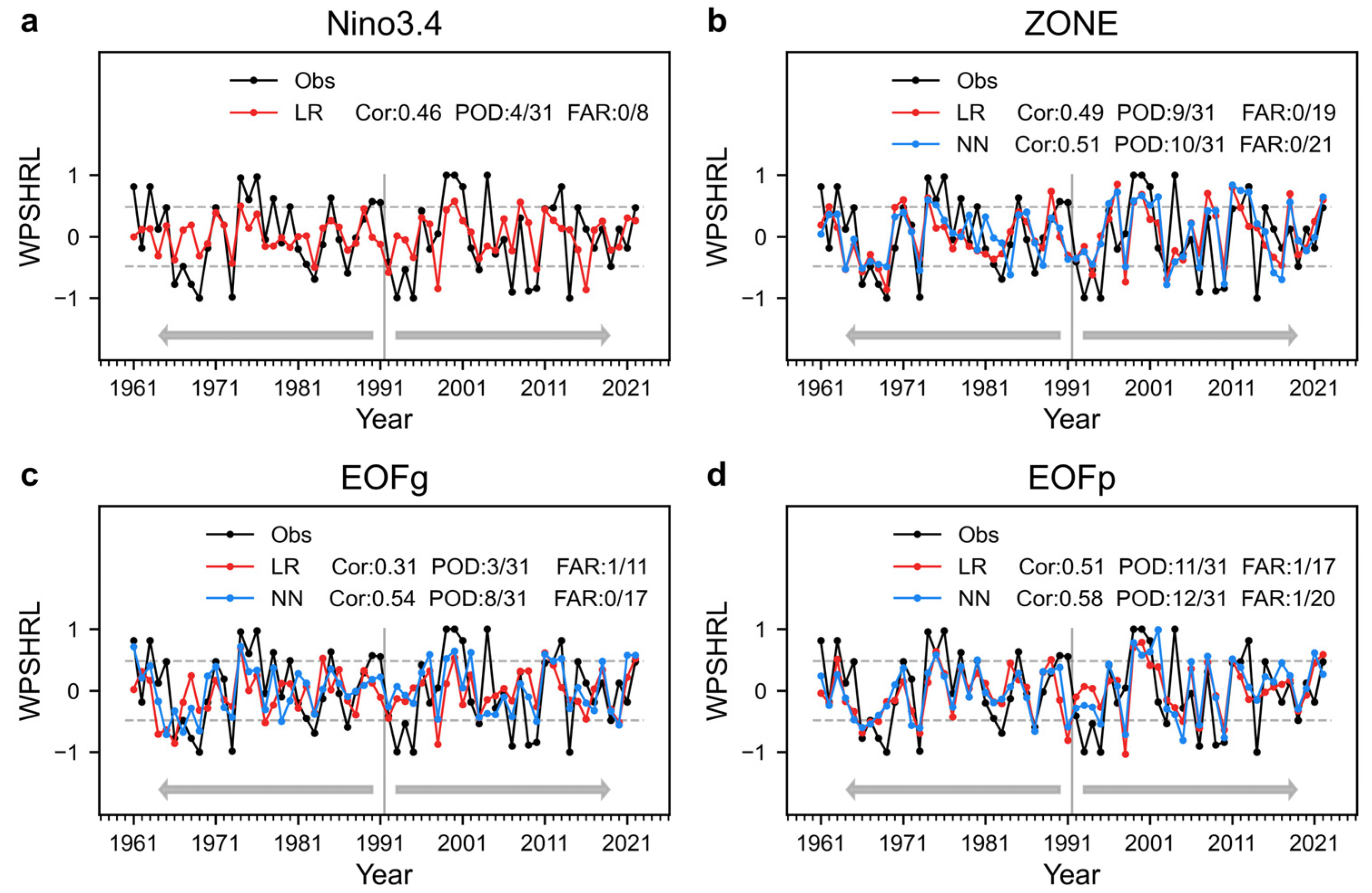
Figure 5 shows the influence of SST extracting methods on forecast skills. The LR experiments (i.e., based on the LR framework) show that one SST predictor (i.e., Niño3.4 index) could give a not-bad forecast once this predictor has a strong correlation with WPSHRL. The Niño3.4 experiment gives a better forecast skill (Cor 0.46, POD 4/31, FAR 0/8) than that from the EOFg experiment (Cor 0.31, POD 3/31, FAR 1/11). The main reason is that those SST areas without any indicative signals are put into every EOFg predictor (the entire global oceans). Unlike the EOFg predictors, the EOFp predictors do not have this disadvantage because they focus on the predominant signal regions (Pacific and Indian oceans). Therefore, the EOFp experiment improves the LR forecast skill (Cor 0.51, POD 11/31, FAR 1/17). The forecast skill from the LR experiment with ZONE predictors (Cor 0.49, POD 9/31, FAR 0/19) is also much better than that with EOFg predictors. One main reason is that only a few ZONE predictors significantly related to WPSHRL are incorporated into the LR forecast models even though these 20 zones are distributed globally. In summary, multiple SST predictors include not only more indicative signals but also more useless signals. As compared to a single strong predictor, the LR forecast skill based on multiple predictors might be improved due to more indicative signals. On the contrary, the forecast skill might worsen if too many useless signals are incorporated into the predictors.

The forecast performance of three multiple-predictor methods under two forecast frameworks are compared in Figure 5b–d. Both are based on the EOFg predictors, the forecast skill from NN models (Cor 0.54, POD 8/31, FAR 0/17) is much better than that from LR models (Cor 0.31, POD 3/31, FAR 1/11). It seems that the NN model can reduce the impact of useless signals mixed in the EOFg SST predictors. The ZONE and EOFp experiments also show that the forecast skills from NN models (Cor 0.51, POD 10/31, FAR 0/21; Cor 0.58, POD 12/31, FAR 1/20) are higher than those from LR models (Cor 0.49, POD 9/31, FAR 0/19; Cor 0.51, POD 11/31, FAR 1/17), especially for anomaly events. Taken overall, these analyses are consistent with previous studies, indicating that the NN model is more effective at exploiting the information provided by input predictors. Regarding the NN framework, there is a certain difference between the forecast skills of the ZONE and EOFp experiments. This might be caused by the fact that the EOFp SST predictors (the Pacific and Indian oceans) contain more information than the ZONE predictors (six zones in Figure 3a), and the orthogonal EOFp SST predictors are relatively easier to use. Taken overall, as compared to the LR models, the NN models could provide higher forecast skills and the differences in the NN forecast skills caused by multiple-predictor extracting methods (i.e., ZONE, EOFg, and EOFp) become small.

4.2. Sensitivity Analysis

The forecast skills only estimate the forecast system from the perspective of the final output predictands. Moreover, the relationship between the input predictors and the output predictand, which is characterized by the regression equation (i.e., the forecast model), constitutes an equally significant consideration. Here, the input–output relationships are investigated by the sensitivities of WPSHRL to the SST field, which can be calculated based on the established forecast model (i.e., model parameters have been determined). During the rolling forecast experiment, the forecast model undergoes an annual update (i.e., the model parameters differ each year) since the available samples used for model establishment are perpetually updated. Consequently, the sensitivity calculated based on the forecast model likewise demonstrates year-to-year variation.

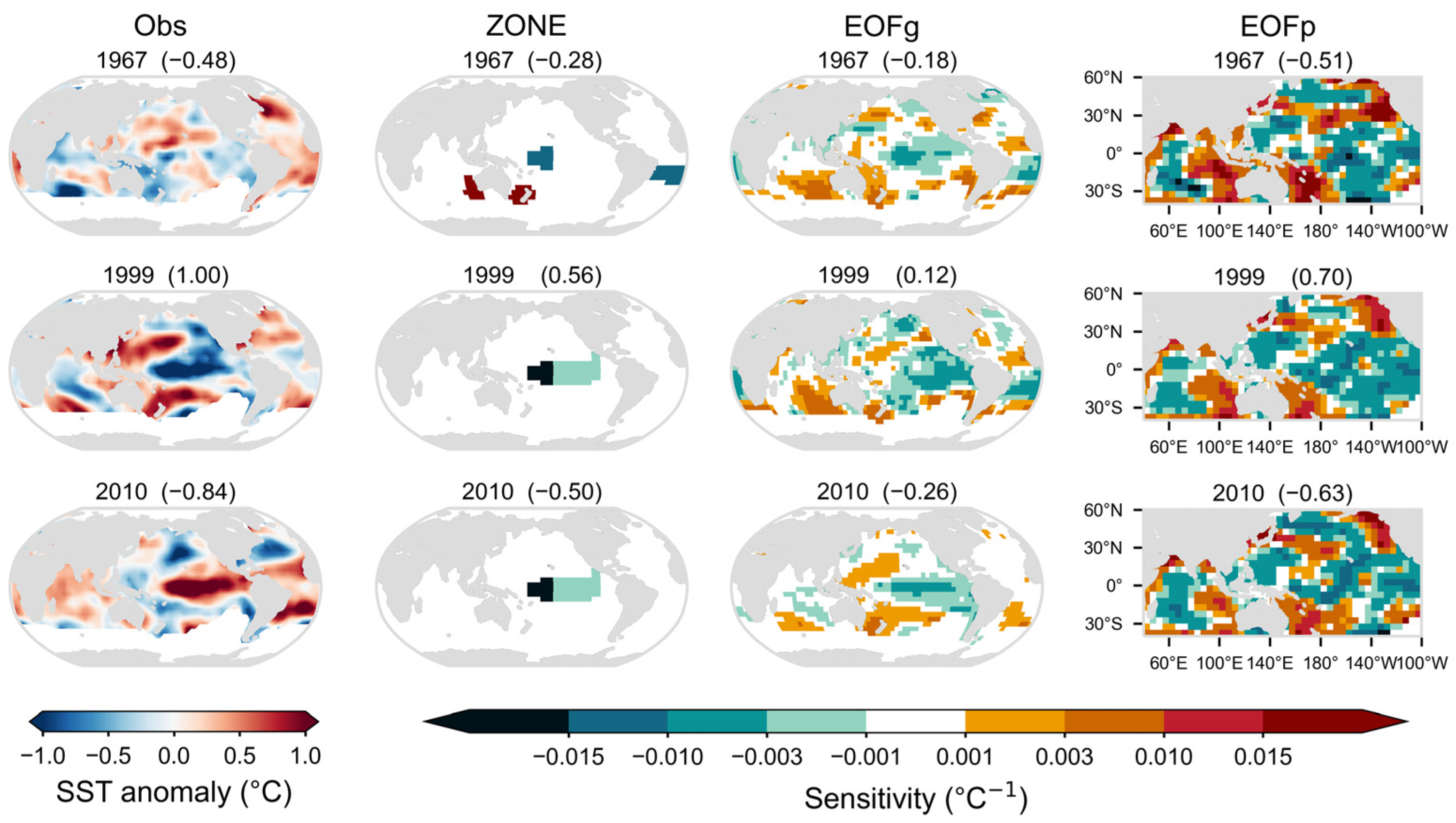
The sensitivities derived from the LR forecast models of three years are presented in Figure 6. Typically, a handful of predictors are selected via the stepwise regression approach, and the predictors employed in the forecast model usually vary from year to year (Figure A2). This phenomenon is manifested in the ZONE experiments. Take the year 2010 as an example, two zones are used in the forecast model. The sensitivities of these two zones are negative, and the two ZONE predictors (i.e., observed SST) exhibit positive values. The inner product of input predictors and corresponding sensitivities determines the value of the output predictand (−0.50, a negative value). The sensitivities from the ZONE experiments indicate that the indicative information predominantly stems from the central-eastern equatorial Pacific region. This is in agreement with the highly correlated regions illustrated in Figure 2. Similarly, in the EOFg and EOFp experiments, the predicted value of WPSHRL is equivalent to the inner product of the observed SST field and the corresponding sensitivity field. Owing to the disparity in the spatial area between the EOFg and EOFp modes, the sensitivity fields from EOFg experiments are comparatively weak and fail to highlight the role of the central-eastern equatorial Pacific region. Consequently, in years with significant abnormalities (e.g., the years 1967 and 1999), the predicted WPSHRLs from the EOFg experiments are substantially weaker than those from the EOFp experiments. This constitutes the primary cause for why the LR experiment with EOFg predictors gives the poorest forecast skill in Figure 5. Overall, the SST-WPSHRL relationships represented by the sensitivity fields in Figure 6 exhibit certain differences among themselves; nonetheless, none of these relationships violate the linear statistical characteristic shown in Figure 2 (i.e., the common pattern from most years).

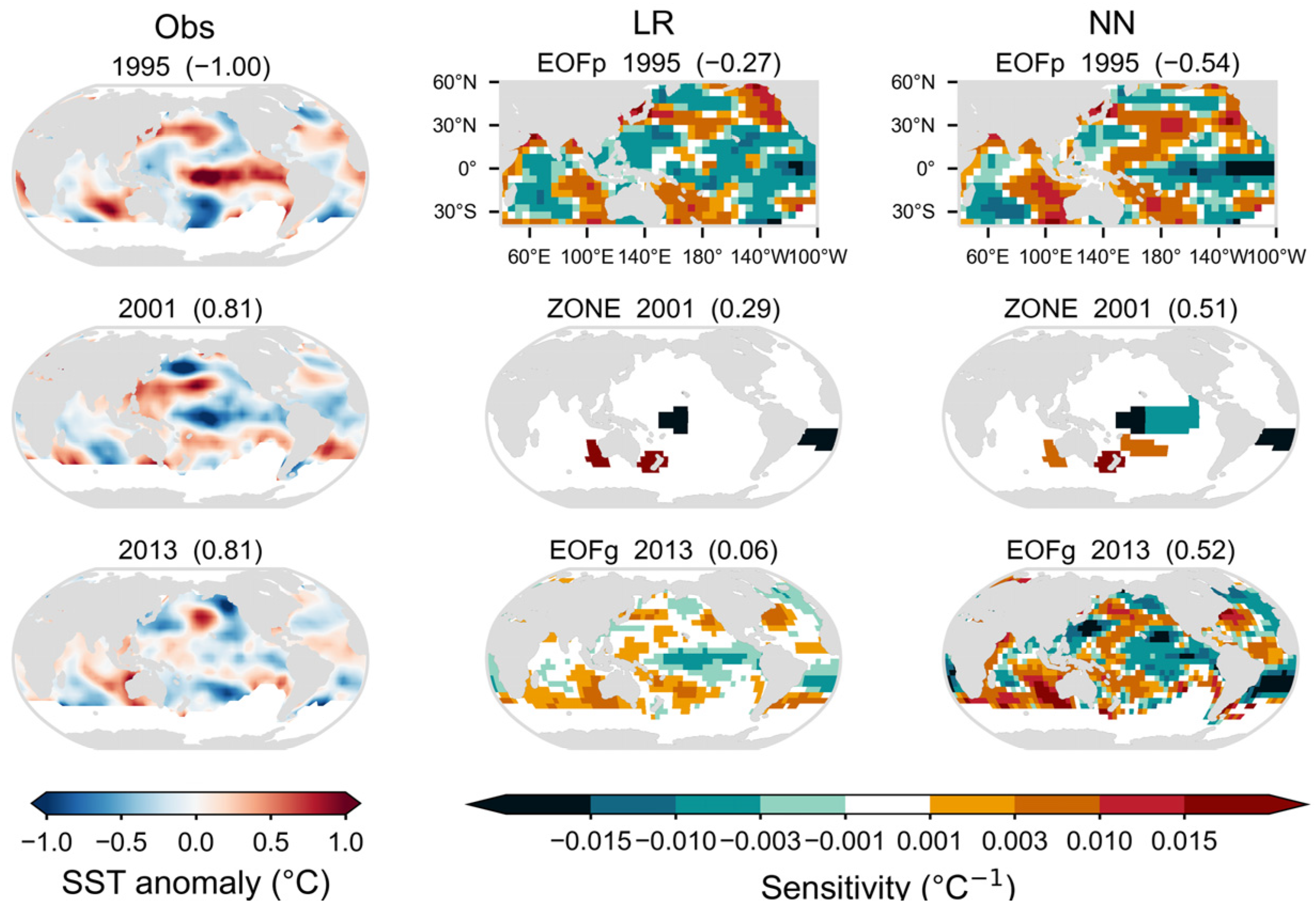
Unlike the sensitivity from LR models, which only depends on LR models themselves, the sensitivity from NN models also depends on the input predictors’ state (i.e., the SST field used for the predicted year). For instance, in one established NN model, the Niño3.4 region sensitivity is influenced by the values of input SST over both the Niño3.4 region and other regions. This is consistent with the fact that the NN model can exploit more SST information for prediction (e.g., the coordination of each predictor). Figure 7 presents a comparison between LR models and NN models. In reference to the 1995 EOFp experiments, the sensitivity pattern from the NN model is somewhat similar to that from the LR model. Nevertheless, the NN model sensitivity is stronger than the LR model sensitivity, particularly over the central-eastern equatorial Pacific (the preceding SST indicative signal is very strong over there). Consequently, the NN model predicts a strong WPSHRL in comparison with the LR model. For the same reason, the 2013 EOFg experiments show a more obvious comparison between the LR model and the NN model. Regarding the 2001 ZONE experiments, both LR and NN models show positive sensitivity over the eastern Indian Ocean near Australia. The preceding negative SST in this region induces a negative WPSHRL. In comparison with the LR model, the less positive NN model sensitivity is one reason for the higher WPSHRL predicted by the NN model. This also suggests that the NN model could flexibly incorporate the preceding SST information, subsequently improving the predicted WPSHRL.

5. Discussion

In this study, the predicted object (i.e., output predictand) is an atmospheric circulation index. To test the robustness of the research conclusions here, we also conducted experiments based on other predictive objects (e.g., the July precipitation over the middle-lower reaches of the Yangtze River). Compared to the WPSHRL, the influence of the SST predictor extracting method is similar, although the forecast skills are decreased to some extent.

6. Conclusions

This study aims to provide valuable insights into extracting SST predictors for the statistical climate forecast system. Within the same climate forecast system, a comparison is made among different methods of extracting SST predictors. To improve the robustness of research conclusions, two kinds of commonly used forecast models are employed in the climate forecast system: linear regression (LR) model and neural network (NN) model. This study investigates four predictor extracting methods: one single-predictor method (Niño3.4 index) and three multiple-predictor methods. The multiple predictors extracted from the EOF approach are orthogonal. In contrast to the multiple predictors extracted from the Pacific and Indian oceans, the multiple predictors extracted from the entire global oceans contain much more useless information for climate forecasting. Unlike the EOF approach, the multiple predictors extracted from the ZONE approach are non-orthogonal but have clear physical meaning.

As compared to a single strong SST predictor, multiple SST predictors contain not only more useful indicative information but also more useless information. Consequently, while multiple SST predictors can offer more information in comparison to a single predictor, the LR forecast model struggles to fully exploit this advantage. Meanwhile, the forecast skill from the LR model is sensitive to the choice of multiple-predictor extracting methods. A primary determinant is whether these multiple predictors contain high quality information, so that the useful information far outweighs the useless information. Unlike the LR model, the NN model shows lower sensitivity to extracting methods because the NN model has a greater capacity in exploiting the useful information provided by input predictors. Moreover, the NN model could provide better forecast skills, especially for anomaly events. The comparison among these three sets of multiple predictors also suggests that whether multiple SST predictors are orthogonal might affect forecast skills. Among these three sets of multiple predictors investigated in this study, the orthogonal multiple predictors extracted from high-quality information regions show the best performance. In conclusion, this study offers valuable insights into the establishment of statistical climate forecast systems based on preceding SST data.

References

- Zhou, T.; Yu, R. Atmospheric water vapor transport associated with typical anomalous summer rainfall patterns in China. J. Geophys. Res. Atmos. 2005, 110, D8. [Google Scholar] [CrossRef]
- Ault, T.R.; Cole, J.E.; Evans, M.N.; Barnett, H.; Abram, N.J.; Tudhope, A.W.; Linsley, B.K. Intensified decadal variability in tropical climate during the late 19th century. Geophys. Res. Lett. 2009, 36, L08602. [Google Scholar] [CrossRef]
- Ren, H.; Zhang, F.; Luo, J.; Wang, R.; Liu, M.; Zhang, W.; Zhou, T.; Zhou, G. A Review of Research on Tropical Air-Sea Interaction, ENSO dynamics, and ENSO prediction in China. J. Meteorol. Res. 2020, 34, 43–62. [Google Scholar] [CrossRef]
- McPhaden, M.J.; Zebiak, S.E.; Glantz, M.H. ENSO as an integrating concept in earth science. Science 2006, 314, 1740–1745. [Google Scholar] [CrossRef]
- Chen, L.; Yuan, Y.; Yang, M.; Zuo, J.; Li, W. A review of physical mechanisms of the global SSTA impact on EASM. J. Appl. Meteorol. Sci. 2013, 24, 521–532. (In Chinese) [Google Scholar]
- Wang, H.; Ren, H.; Chen, H.; Ma, J.; Tian, B.; Sun, B.; Huang, Y.; Duan, M.; Wang, J.; Wang, L. Highlights of climate prediction study and operation in China over the past decades. Acta Meteorol. Sin. 2020, 78, 317–331. (In Chinese) [Google Scholar]
- Ding, Y. Progress and prospects of seasonal climate prediction. Adv. Meteorol. Sci. Technol. 2011, 1, 14–27. (In Chinese) [Google Scholar]
- Wei, F. Physical basis of short-term climate prediction in China and short-term climate objective prediction methods. J. Appl. Meteorol. Sci. 2011, 22, 1–11. (In Chinese) [Google Scholar]
- Kosaka, Y.; Chowdary, J.S.; Xie, S.; Min, Y.; Lee, J. Limitations of seasonal predictability for summer climate over East Asia and the Northwestern Pacific. J. Clim. 2012, 25, 7574–7589. [Google Scholar] [CrossRef]
- Zhou, B.; Wang, H. Relationship between the boreal spring Hadley circulation and the summer precipitation in the Yangtze River valley. J. Geophys. Res. 2006, 111, 1–14. [Google Scholar] [CrossRef]
- Yun, K.; Seo, K.; Ha, K. Relationship between ENSO and northward propagating intraseasonal oscillation in the east Asian summer monsoon system. J. Geophys. Res. Atmos. 2008, 113, D14. [Google Scholar] [CrossRef]
- Jiang, W.; Huang, G.; Huang, P.; Wu, R.; Hu, K.; Chen, W. Northwest Pacific anticyclonic anomalies during post-El Niño summers determined by the pace of El Niño decay. J. Clim. 2019, 32, 3487–3503. [Google Scholar] [CrossRef]
- Huang, R.; Wu, Y. The influence of ENSO on the summer climate change in China and its mechanism. Adv. Atmos. Sci. 1989, 6, 21–32. [Google Scholar] [CrossRef]
- Wang, B.; Wu, R.; Fu, X. Pacific-East Asian teleconnection: How does ENSO affect east Asian climate? Am. Meteorol. Soc. 2000, 13, 1517–1536. [Google Scholar] [CrossRef]
- Lin, Z.; Lu, R. The ENSO’s effect on eastern China rainfall in the following early summer. Adv. Atmos. Sci. 2009, 26, 333–342. [Google Scholar] [CrossRef]
- Wei, F. Progresses on climatological statistical diagnosis and prediction methods-in commemoration of the 50 anniversaries of CAMS establishment. J. Appl. Meteorol. Sci. 2006, 17, 736–742. (In Chinese) [Google Scholar]
- Cao, J.; Lu, R.; Hu, J.; Wang, H. Spring Indian Ocean-Western Pacific SST contrast and the East Asian summer rainfall anomaly. Adv. Atmos. Sci. 2013, 30, 1560–1568. [Google Scholar] [CrossRef]
- Zhao, H. Analysis and prediction of the spatiotemporal characteristics of the interaction between the subtropical high and sea surface temperature. Meteorol. Mon. 1986, 12, 21–23. (In Chinese) [Google Scholar]
- Chen, C.; Georgakakos, A.P. Seasonal prediction of East African rainfall. Int. J. Climatol. 2015, 35, 2698–2723. [Google Scholar] [CrossRef]
- Liu, Y.; Fan, K. A new statistical downscaling model for autumn precipitation in China. Int. J. Climatol. 2013, 33, 1321–1336. [Google Scholar] [CrossRef]
- Zhang, W.; Jin, F.; Stuecker, M.F.; Andrew, T.; Wittenberg, A.T.; Ren, H.; Kug, J.; Cai, W.; Cane, M. Unraveling El Nino’s impact on the East Asian monsoon and Yangtze River summer flooding. Geophys. Res. Lett. 2016, 43, 11375–11382. [Google Scholar] [CrossRef]
- Qian, D.; Guan, Z.; Xu, J. Prediction models for summertime Western Pacific Subtropical High based on the leading SSTA modes in the tropical Indo-Pacific sector. Trans. Atmos. Sci. 2021, 44, 405–417. (In Chinese) [Google Scholar]
- Huang, C.; Li, Q.; Xie, Y.; Peng, J. Prediction of summer precipitation in Hunan based on machine learning. Trans. Atmos. Sci. 2022, 45, 191–202. (In Chinese) [Google Scholar]
- Sun, C.; Shi, X.; Yan, H.; Jiang, Q.; Zeng, Y. Forecasting the June Ridge Line of the Western Pacific Subtropical High with a Machine Learning Method. Atmosphere 2022, 13, 660. [Google Scholar] [CrossRef]
- Jiang, Q.; Shi, X. Forecasting the July Precipitation over the middle-lower reaches of the Yangtze River with a flexible statistical model. Atmosphere 2023, 14, 152. [Google Scholar] [CrossRef]
- Kaplan, A.; Cane, M.A.; Kushnir, Y.; Clement, A.C.; Blumenthal, M.B.; Rajagopalan, B. Analyses of global sea surface temperature 1856–1991. J. Geophys. Res. 1998, 103, 18567–18589. [Google Scholar] [CrossRef]
- Liu, Y.; Li, W.; Ai, W.; Li, Q. Reconstruction and application of the monthly western Pacific subtropical high indices. J. Appl. Meteorol. Sci. 2012, 23, 414–423. (In Chinese) [Google Scholar]
- Chen, L. Interaction between the subtropical high over the north pacific and the sea surface temperature of the eastern equatorial pacific. Sci. Atmos. Sin. 1982, 6, 148–156. (In Chinese) [Google Scholar]
- Zhao, Z.; Chen, G. The cause and forecast of long-term change of the latitudinal position of west pacific subtropical high in early summer. J. Trop. Meteorol. 1995, 11, 223–230. (In Chinese) [Google Scholar]
- Ying, M.; Sun, S. A study on the response of subtropical high over the Western Pacific on the SST anomaly. Chin. J. Atmos. Sci. 2000, 24, 193–206. (In Chinese) [Google Scholar]
- Yao, Y.; Yan, H. Relationship between proceeding pacific sea surface temperature and subtropical high indexes of main raining seasons. J. Trop. Meteorol. 2008, 24, 483–489. (In Chinese) [Google Scholar]
- Kim, J.E.E.; Yoo, C.; Park, S.H. Interdecadal change in the relationship between the western North Pacific subtropical high and the ENSO. Theor. Appl. Climatol. 2023, 151, 1435–1447. [Google Scholar] [CrossRef]
- Zhang, R.; Jiang, G.; Yu, Z.; Jiang, Q. Establishment of prediction model for the pacific subtropical high using neural network calculation method. Q. J. Appl. Meteorol. 2000, 11, 474–483. (In Chinese) [Google Scholar]
- Qian, D.; Guan, Z.; Tang, W. Joint impacts of SSTA in tropical Pacific and Indian Oceans on variations of the WPSH. J. Meteorol. Res. 2018, 32, 548–559. [Google Scholar] [CrossRef]
- Wu, X.; Guo, S.; Ba, H.; He, S.; Xiong, F. Long-range precipitation forecasting based on multipole sea surface temperature. ShuiLi XueBao 2018, 49, 1276–1283. (In Chinese) [Google Scholar]
- Richman, M.B. Principal component analysis in meteorology and oceanography. Am. Meteorol. Soc. 1990, 71, 212–214. [Google Scholar]
- Storch, H.; Zwiers, F.W.; Livezey, R.E. Statistical analysis in climate research. Nature 2000, 404, 544. [Google Scholar]
- Mo, R.; Straus, M.D. Statistical-dynamical seasonal prediction based on principal component regression of GCM ensemble integrations. Am. Meteorol. Soc. 2002, 130, 2167–2187. [Google Scholar] [CrossRef]
- Zhang, J.; Zhao, Q.; Xu, X. Methods for Combining Predictors in Statistical Forecasting. Sci. Atmos. Sin. 1978, 2, 48–54. (In Chinese) [Google Scholar]
- Wilks, D.S. Statistical Methods in the Atmospheric Sciences, 3rd ed.; Academic Press: London, UK, 2006; pp. 235–312. [Google Scholar]
- Derksen, S.; Keselman, H.J. Backward, forward and stepwise automated subset selection algorithms: Frequency of obtaining authentic and noise variables. Br. J. Math. Stat. Psychol. 1992, 45, 265–282. [Google Scholar] [CrossRef]
- Kutner, M.H.; Nachtsheim, C.J.; Neter, J.; Li, W. Applied Linear Statistical Models; McGrawhill: New York, NY, USA, 2005. [Google Scholar]
- Goodfellow, I.; Bengio, Y.; Courville, A. Deep Learning; MIT Press: Cambridge, CA, USA, 2016; pp. 89–223. [Google Scholar]
- Dodge, J.; Ilharco, G.; Schwartz, R.; Farhadi, A.; Hajishirzi, H.; Smith, N. Fine-tuning pretrained language models: Weight initializations, data orders, and early stopping. arXiv 2020, arXiv:2002.06305. [Google Scholar] [CrossRef]
- Snieder, E.; Abogadil, K.; Khan, U.T. Resampling and ensemble techniques for improving ANN-based high-flow forecast accuracy. Hydrol. Earth Syst. Sci. 2021, 25, 2543–2566. [Google Scholar] [CrossRef]
- Mao, W.; Chen, Y.; Bai, S.; Li, W. Experiment of running prediction of precipitation in flood period in China with ensemble analysis of physical-statistic prediction. Meteorol. Mon. 2011, 37, 547–554. (In Chinese) [Google Scholar]
- Huang, X.; He, L.; Zhao, H.; Huang, Y.; Wu, Y. Application of shapley-fuzzy neural network method in long-time rolling forecasting of typhoon satellite image in South China. Acta Meteorol. Sin. 2021, 79, 309–327. (In Chinese) [Google Scholar] [CrossRef]
- Tian, W.; Song, P.; Chen, Y. Short-term rolling prediction of tropical cyclone intensity based on multi-task learning with fusion of deviation-angle variance and satellite imagery. Adv. Atmos. Sci. 2024, 42, 111–128. [Google Scholar] [CrossRef]
- Zhu, C.; Park, C.K.; Lee, W.S.; Yun, W.T. Statistical downscaling for multi-model ensemble prediction of summer monsoon rainfall in the Asia-Pacific region using geopotential height field. Adv. Atmos. Sci. 2008, 25, 867–884. [Google Scholar] [CrossRef]
- Ke, Z.; Zhang, P.; Dong, W.; Wang, J. An application of optimal subset regression in seasonal climate prediction. Chin. J. Atmos. Sci. 2009, 33, 994–1002. (In Chinese) [Google Scholar]
- Ren, H.L.; Jin, F.F.; Song, L.; Lu, B.; Tian, B.; Zuo, J.; Liu, Y.; Wu, J.; Zhao, C.; Nie, Y.; et al. Prediction of primary climate variability modes at the Beijing Climate Center. J. Meteorol. Res. 2017, 31, 204–223. [Google Scholar] [CrossRef]
- Liu, Y.; Ren, H.; Zhang, P.; Zuo, J.; Tian, B.; Wan, J.; Li, Y. Application of the hybrid statistical downscaling model in summer precipitation prediction in China. Clim. Environ. Res. 2020, 25, 163–171. Available online: http://www.iapjournals.ac.cn/qhhj/cn/article/pdf/preview/10.3878/j.issn.1006-9585.2019.18168.pdf (accessed on 10 January 2025). (In Chinese).
- Chen, F.; Li, X. Evaluation of IMERG and TRMM 3B43 monthly precipitation products over mainland China. Remote Sens. 2016, 8, 472. [Google Scholar] [CrossRef]
- Chen, C.; Chen, Q.; Duan, Z.; Zhang, J.; Mo, K.; Li, Z.; Tang, G. Multiscale comparative evaluation of the GPM IMERG v5 and TRMM 3B42 v7 precipitation products from 2015 to 2017 over a climate transition area of China. Remote Sens. 2018, 10, 944. [Google Scholar] [CrossRef]
- Frnda, J.; Durica, M.; Nedoma, J.; Zabka, S.; Martinek, R.; Kostelansky, M. A weather forecast model accuracy analysis and ECMWF enhancement proposal by neural network. Sensors 2019, 19, 5144. [Google Scholar] [CrossRef]