Article

Characteristics of Aerosol Number Concentration Power Spectra and Their Influence on Flux Measurements

1
School of Mathematics and Physics, Anhui Jianzhu University, Hefei 230601, China
2
School of Earth and Space Science, University of Science and Technology of China, Hefei 230026, China
*
Author to whom correspondence should be addressed.
Atmosphere 2025, 16(3), 332; https://doi.org/10.3390/atmos16030332
Submission received: 10 January 2025 / Revised: 28 February 2025 / Accepted: 12 March 2025 / Published: 15 March 2025
(This article belongs to the Section Aerosols)

Abstract

:
In this paper, a water-based aerosol particle counter was used to measure aerosol number concentrations with high temporal resolution at a meteorological tower and on the ground, and the ultrasonic anemometer on the meteorological tower measured the data of the three-dimensional wind speed. The power spectrum of the aerosol particle number concentration fluctuation was obtained by using a Fourier transform, and the characteristics of the power spectrum were deeply analyzed. The results show that the aerosol concentration fluctuation power spectrum satisfies the Monin–Obukhov law in the low-frequency (0.02–0.25 Hz) part of the inertial subregion, which is consistent with the characteristics of atmospheric turbulent motion. Significant attenuation occurs in the high-frequency (0.3–5 Hz) range, which is mainly caused by the attenuation of the aerosol concentration by the intake pipe. Using the similarity of the power spectrum in the low-frequency part, using the “−5/3” line as a standard, the characteristic time of the measurement system is obtained by fitting the transfer function. The results show that in the flux measurement experiments in this paper, the characteristic time is usually less than 1 s. Finally, this paper uses the Fourier transform and wavelet transform to correct the high-frequency attenuation in the fluctuation of aerosol concentration and obtains the corrected aerosol flux. The results show that the effect of high-frequency attenuation on the flux is approximately 1–4% in this experiment.

1. Introduction

Aerosols are important pollutants in the atmosphere, not only affecting climate change but also having a significant impact on human health [1,2]. Various methods such as the eddy covariance, gradient method, relaxed eddy accumulation, mass balance method, and large aperture scintillator are used to observe changes in aerosol concentrations and emissions [3,4,5]. Among them, the eddy correlation method and large aperture scintillator are the two main methods, which can obtain accurate real-time aerosol emission data [6]. Using a large aperture scintillometers to observe aerosol flux requires the assumption that aerosol concentration, like other scalar gasses such as CO2, conforms to the motion law of atmospheric turbulence and satisfies the Monin–Obukhov law which is a “−5/3” slope in the inertial subregion of the power spectrum [7,8,9]. In fact, aerosols are mixed in the atmosphere in the form of particles, and physical processes and chemical reactions take place frequently [10]. Atmospheric conditions affect these physical processes and chemical reactions and thus the concentration of aerosols. For example, radiation will affect the generation of new particles, humidity will affect the hygroscopic process of hydrophilic aerosols, wind direction, and speed, and atmospheric stability will change the concentration of aerosols at the observation point by affecting the source area of the aerosol. Rapid changes in these meteorological conditions can affect aerosol concentrations to varying degrees [3,11]. Observations in the Amazon basin and Stockholm show that the aerosol power spectrum satisfies the “−5/3” law in the inertial subregion according to Kolmogorov’s similarity theory within a certain margin of error [12,13]. The cause of the deviation of the power of aerosol number concentration from the Monin–Obukhov law is still not clear. Therefore, whether the changes in the aerosols in the atmosphere conform to the law of scalar motion still needs to be further studied.
The eddy correlation method (EC) has been widely used in the measurement of mass flux and energy flux [14], and in recent years, it has also been used in the measurement of aerosol flux. The EC system is usually a closed circuit or semi-open circuit, and the air is drawn into the instrument through the intake pipe to measure the concentration of the aerosol [15]. Aerosol flux observation experiments were carried out in Stockholm [13] and Helsinki [16]. The intake ducts used were 10 m and 40 m long and 1/4 inch and 8 mm in diameter. Aerosol particle deposition observations were carried out in the Amazon rainforest [12]. The air intake pipe used was 2.5 m long and had an inner diameter of 1/4 inch. In the flux observation experiment, due to the effect of the intake pipe, the measured power spectrum will inevitably be affected by the intake pipe, which will correspondingly affect the fluctuation intensity of the aerosol and introduce errors to the flux measurement. Therefore, in the measurement of aerosol flux, it was necessary to analyze the characteristics of the aerosol concentration power spectrum and to correct the error of the aerosol flux. At present, the effect of closed-loop eddy-correlated systems on high frequencies is usually represented by a transfer function [15,17,18]. The observations of fluxes are often accompanied by noise, and noisy signals can affect the calculation of the transfer function. Ibrom et al. removed the noise signal before calculating the characteristic time [19]. Aslan et al. further developed a method for directly fitting noisy signals [14]. Correction using a wavelet transform on the high-frequency part of the power spectrum compensates for an underestimation in water vapor flux measurements [20]. This study shows that in the measurement of aerosol flux, the aerosol concentration fluctuation spectrum also has attenuation in the high-frequency part. Enroth et al. measured the characteristic time of a condensation particle counter in laboratory [21]. Oosterwijk et al. discussed the attenuation and correction of aerosol spectra in aerosol flux measurements and used different fitting schemes to quantitatively describe the high-frequency attenuation in two aerosol flux measurement experiments [22]. The results show that the aerosol flux is attenuated by 4–35% in the measurement. The study concluded that only spectral densities greater than the peak frequency would be affected by the intake duct. In fact, the intake duct has an impact on the spectral density at all frequencies, and the impact of low frequencies is relatively small compared to high frequencies, but it cannot be completely ignored.
In this paper, by carrying out aerosol flux observation experiments, the characteristics of the fluctuation spectrum of aerosol concentration in the atmosphere are studied and analyzed, the high-frequency attenuation caused by the intake pipe is calculated, and the high-frequency flux loss is compensated by Fourier transform and wavelet transform. The effect of high-frequency attenuation on flux measurements is obtained. The experimental conditions and data processing methods are described in Section 2. The basic characteristics of the spectrum are given in Section 3.1. In Section 3.2, the high-frequency attenuation was compensated by two methods, and the corrected aerosol flux was obtained.

2. Experiment and Data Processing Methods

2.1. Experiment

The experimental site is located on the roof of a 4-story building on the campus of the University of Science and Technology of China, Hefei, Anhui Province, China. A three-dimensional ultrasonic anemometer and a condensation particle counter were used to carry out aerosol vertical flux observation experiments on a meteorological tower. Two observation experiments were carried out in different time periods. Another control experiment was carried out at 1 m above the bottom of the tower without the intake pipe. The experimental conditions are shown in Table 1.
As a comparison, in Experiment 2, aerosol number concentration observations were carried out on the ground for a long time to obtain the characteristics of aerosol concentration fluctuations when the intake pipe was not connected. In experiment 2, a comparative experiment was carried out. In the ground observation, the intake pipe was first connected for one hour, and then the intake pipe was removed and observed for one hour, repeated several times to obtain the influence of the aerosol number concentration power spectrum caused by the intake duct under similar atmospheric conditions.
The tower is located on the top of the 4-story building, and its bottom end is 3 m above the canopy level. Two ultrasonic anemometers of type CSAT3 were installed on the top of the tower, the sampling frequency is 10 Hz, and they were located 15 and 18 m away from the bottom of the tower to ensure reliable data for comparative analysis. Five levels of RM Young 03002 anemometers and HMP155A temperature and humidity sensors (located at 21 m, 15.5 m, 11 m, 7.5 m, and 5 m above the canopy plane) were also installed on the weather tower to obtain the vertical gradient of wind speed, wind direction, air temperature, and air relative humidity. At the same time, a four-component radiometer was installed at a distance of 8 m from the bottom of the tower. The time resolution was 1 min.
The aerosol particle number concentration was measured by a TSI3788 water-based condensate particle counter produced by TSI Corporation (Shoreview, MN, USA). The sampling frequency of the instrument is up to 10 Hz, and the smallest detectable particle size is 2.5 nm. Using this instrument, rapid changes in particle number concentration can be obtained. To measure the vertical flux of aerosols on the iron tower under all weather conditions, the instrument is installed in a sealed box fixed on the iron tower, approximately 1.5 m from the vertical distance of the ultrasonic anemometer, and air sampling is carried out through a stainless-steel tube. The air inlet with a length of 2 m is 20 cm away from the ultrasonic anemometer, and the inner diameter of the stainless-steel tube is 4 mm.

2.2. Data Quality Control

Since the experiment is conducted outdoors, there are many interference factors in the measurement, and the high-frequency sampling aerosol particle concentration data and three-dimensional wind data often have data outliers, which will affect the results of the experimental observation. To ensure the validity and accuracy of the data, this paper first performs quality inspection and outlier correction on the collected raw data. First, the data are divided into 36,000 pieces of data for 1 h, and the time series Δ x of the difference is obtained by calculating the difference between two adjacent points. The data in this time series that are greater than 4 times the standard deviation belong to the outliers, that is, | Δ x | > 4σ. Here, σ is the standard deviation of the difference series for this hour. When the number of outliers in an hour exceeds 1%, that is, 360 data points, the data for that hour are considered invalid and do not participate in subsequent calculations. When the number of outliers is less than 1%, we use adjacent data points for interpolation and repeat the above process after interpolation until the outliers are completely corrected.

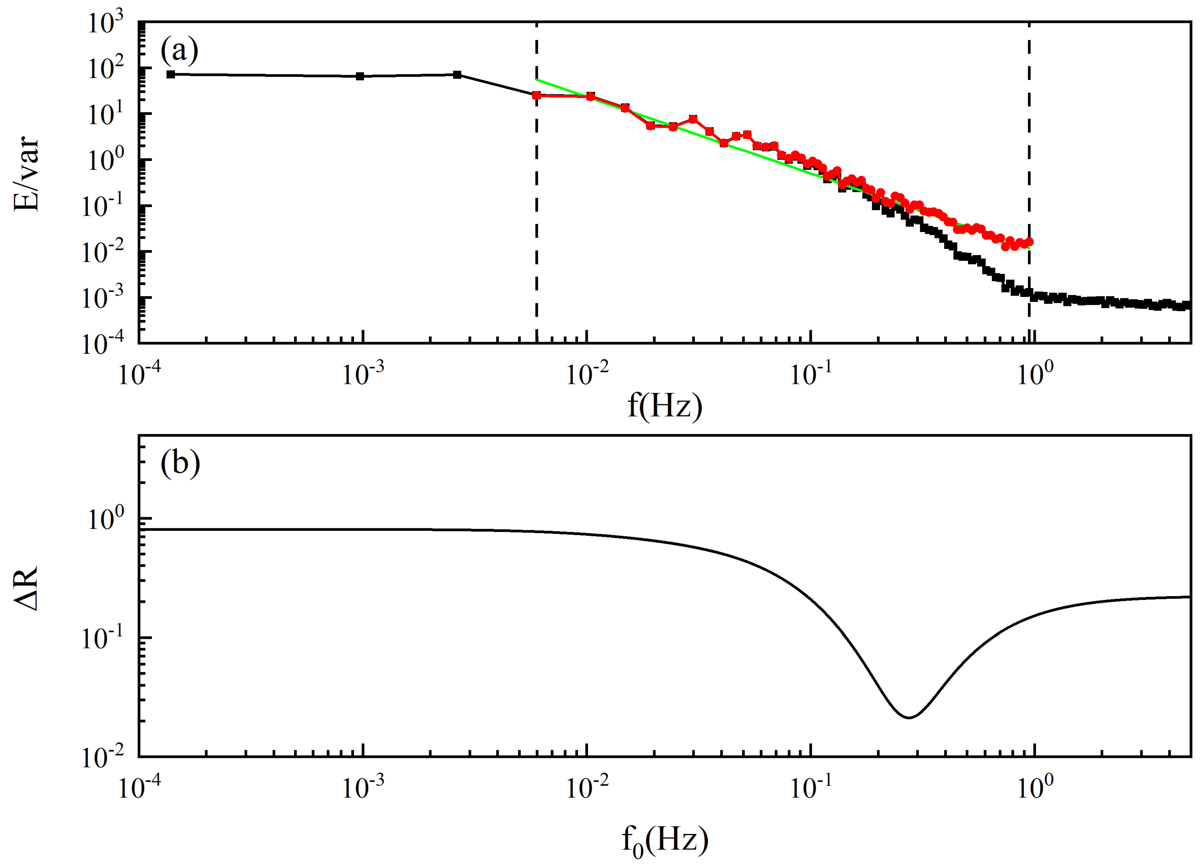
2.3. A Description Method of the High-Frequency Attenuation Characteristics of the Aerosol Concentration Fluctuation Power Spectrum

The aerosol concentration fluctuation power spectrum usually has attenuation at high frequencies. To quantitatively describe the high-frequency attenuation, the aerosol measurement system can be regarded as a measurement system with a first-order delay response, which satisfies
C t = C C τ
where τ is the characteristic time of the measurement system, C is the value measured by the instrument, and C is the actual concentration in the atmosphere. A transfer equation can be derived to describe the attenuation of the spectrum in the measurement system:
T f = 1 1 + 2 π f τ 2
where f is the frequency, and the transfer function can quantitatively describe the high-frequency attenuation of the spectrum. The real aerosol concentration fluctuation spectrum E a f and the observed concentration fluctuation spectrum E m f in the atmosphere should satisfy
T f = E m f E a f
The normalized aerosol power spectrum and the standard spectrum should be roughly the same, that is, E a f N a and E s f N s should be fairly close, where Na and Ns are the integral of the power spectral density within a certain frequency interval.
N a = f 1 f 2 E a f d f
N s = f 1 f 2 E s f d f
Theoretically, the integral interval should be the full frequency domain of the experimental measurement, that is, f 1 = 0 , f 2 = 5   Hz . Since the power spectrum obtained in the actual measurement is always discrete, it needs to be smoothed, and the smoothed power spectrum is represented by E a , t , w n . Since the first few points of the low-frequency part are less smoothed and will be affected by the detrending method, their values are unstable, so in this paper, the lower limit of the integration interval f 1 is set as the fourth point of the smoothed power spectrum, and the value is 0.006 Hz. There is a noise signal in the high-frequency part of the aerosol concentration fluctuation power spectrum, so considering the similarity between the two, it is necessary to remove this part; that is, the upper limit of integration f 2 should be set to the minimum frequency of noise.
When the normalized aerosol power spectrum E s f f 1 f 2 E s f d f and the standard spectrum after transfer function compensation E m f T f f 1 f 2 E m f T f d f are the closest, the corresponding τ is the characteristic time of the measurement system. The calculation process of τ is as follows. For a specific τ , the corresponding transfer function and corrected power spectrum E m f T f are obtained. To quantitatively describe the deviation between the compensated power spectrum and the standard spectrum, the following formula was used to obtain the logarithmic root mean square error Δ R :
Δ R = ( log 10 E A n N A log 10 E S n N S ) 2 ¯
where E A n is the discretized E a f = E m f T f , N A is the integral of the correction interval, and E S n and N S are the same. The τ corresponding to the minimum value of Δ R is the characteristic time required in this paper. f 0 = 1 2 π τ , that is, the frequency at which the T f value is 1/2, and its value can intuitively reflect the attenuation of the power spectrum in the high-frequency range. When f 0 is small, the aerosol power spectrum reaches 1/2 of the standard spectrum at a lower frequency, and it can be considered that the attenuation is stronger. When the value of f 0 obtained by fitting exceeds the minimum frequency of noise occurrence, that is, the attenuation does not reach 1/2 in the effective fitting interval, it can be considered that no attenuation has occurred in the inertial subregion during this time period.

2.4. Correction Methods for High-Frequency Power Spectra of Aerosol Concentration Fluctuation

When performing aerosol flux measurement, to protect the precise aerosol measuring instrument and reduce the interference to the ultrasonic anemometer and the installation requirements, the air extraction measurement is usually carried out through several meters of intake pipes. However, the existence of the intake pipe brings some measurement problems, mainly including the time delay between the ultrasonic anemometer and the aerosol measuring instrument and the attenuation of the aerosol concentration by the intake pipe.
For the time delay, the approximate time delay is calculated by the extraction flow rate, and the exact delay time is determined by the extreme value of the delay of the aerosol concentration and the vertical wind speed. In the measurement, the intake pipe not only attenuates the mean concentration but also attenuates the high-frequency part of the aerosol number concentration fluctuation spectrum. To explore the attenuation of the aerosol concentration fluctuation spectrum by the intake pipe and its influence on the flux measurement, the obvious way is to calculate the aerosol number concentration fluctuation spectrum and flux separately from the aerosol concentration time series before and after passing through the intake pipe. However, in the actual measurement, we lack such measurement conditions, and the particle counter will also interfere with the measurement of the ultrasonic anemometer.
A feasible method is to obtain the unattenuated aerosol concentration time series through the measured aerosol concentration time series. That is, the attenuated high-frequency signal is compensated, and the influence of the intake pipeline on the flux measurement is obtained by comparing the aerosol flux before and after compensation. Since there are no measured aerosol flux data for the unconnected intake pipe, this paper uses two methods to compensate for the high-frequency attenuation for comparison and correction based on the FFT method and the wavelet method for comparison and verification. The parameters that need to be determined in the correction scheme are mainly the lowest frequency of correction and the amplitude of correction in the high-frequency interval.

2.4.1. Correction Based on the FFT Method

As seen previously, the characteristic time can quantitatively characterize the strength of the high-frequency attenuation. Therefore, the transfer function represented by the characteristic time can reversely compensate for the high-frequency attenuation, and the compensation amplitude is the reciprocal of the transfer function.
1 T f = 1 + 2 π f τ 2
The unsmoothed power spectrum will be directly multiplied by the inverse of the transfer function to obtain the compensated power spectrum. It is worth noting that the transfer function is only used for the correction of the inertial subregion, mainly because the noise signal does not contribute to the flux. Different spectra such as the standard spectrum will make the characteristic time different. In this paper, the transfer function obtained by different spectra is used as the compensation amplitude. The compensated aerosol concentration can be obtained from the compensated power spectra through the inverse Fourier transform, and the corrected aerosol flux can be obtained.

2.4.2. Correction Based on the Wavelet-Based Method

Refer to the correction method for water vapor flux [20]. This method performs wavelet transform on aerosol concentrations, compensates for its high-frequency wavelet coefficients, and obtains the corrected sequence through inverse transform. This paper uses the Haar wavelet as the basis function to perform discrete wavelet transform on high-frequency data and obtains the wavelet coefficients W w , C a j , b j , where a j is the wavelet scale factor, b j is the position factor, and the wavelet scale is a j = 2 j , j = 1 : 15 . b j = 2 15 j wavelet coefficients are obtained for each scale, the value of the position factor is [1:215−j], and the frequency corresponding to the scale factor is f j = 2 15 j 2 15 f s , where f s is the sampling frequency. The wavelet spectral density at each scale is determined by the following formula:
P w , C j = W w , C a j , b 2 ¯ f s l n 2
The wavelet scale ( a j 0 ) corresponding to the extreme point of f P w / σ w is set as the lower limit of the high-frequency range that needs to be adjusted; that is, the wavelet coefficient whose scale is larger than a j > a j 0 ( j > j 0 ) in the wavelet coefficient W C a j , b j corresponding to the aerosol concentration needs to be adjusted. The frequency interval whose scale is a j j 0 2 j j 0 will be used as the unattenuated part to obtain the unattenuated spectral density of the high-frequency interval and then determine the adjustment range of the high-frequency interval. A straight line is fitted; when the slope is between [−1.8 and −1.3], it is considered reasonable, and it will be extended to the high-frequency range to obtain an unattenuated spectral density. When outside this range, a straight line with a slope of −5/3 is used as the standard. After determining the interval to be adjusted and the adjustment range, the position factor to be adjusted must be further determined. The intake duct attenuation not only attenuates the magnitude but also affects the phase angle. The position of the wavelet coefficients is also distorted, so all small-scale wavelet coefficients cannot simply be adjusted in a similar manner or proportional to their energy content, which cannot be achieved using Fourier transform adjustment. Then, we select W w a j , b j with larger energy and adjust W C a j , b j with the same scale and location factor. The W w 2 a j , b j in a scale that needs to be adjusted is arranged from large to small, the cumulative contribution of 90% of the total energy of the scale will be determined as the threshold, and the W C a j , b j corresponding to the W w 2 a j , b j that exceeds the threshold will be adjusted. The adjusted wavelet coefficients can reconstruct the fluctuation signal of aerosol concentration through inverse wavelet transform and obtain the corrected aerosol flux.

3. Results

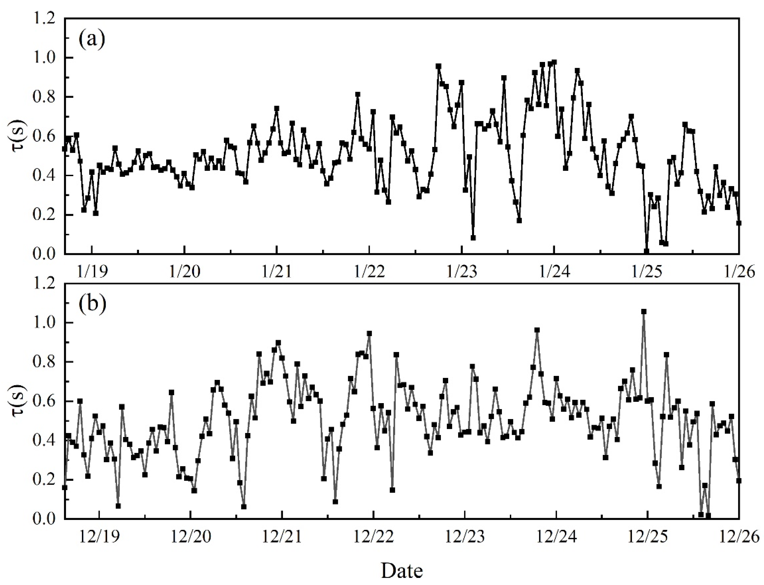
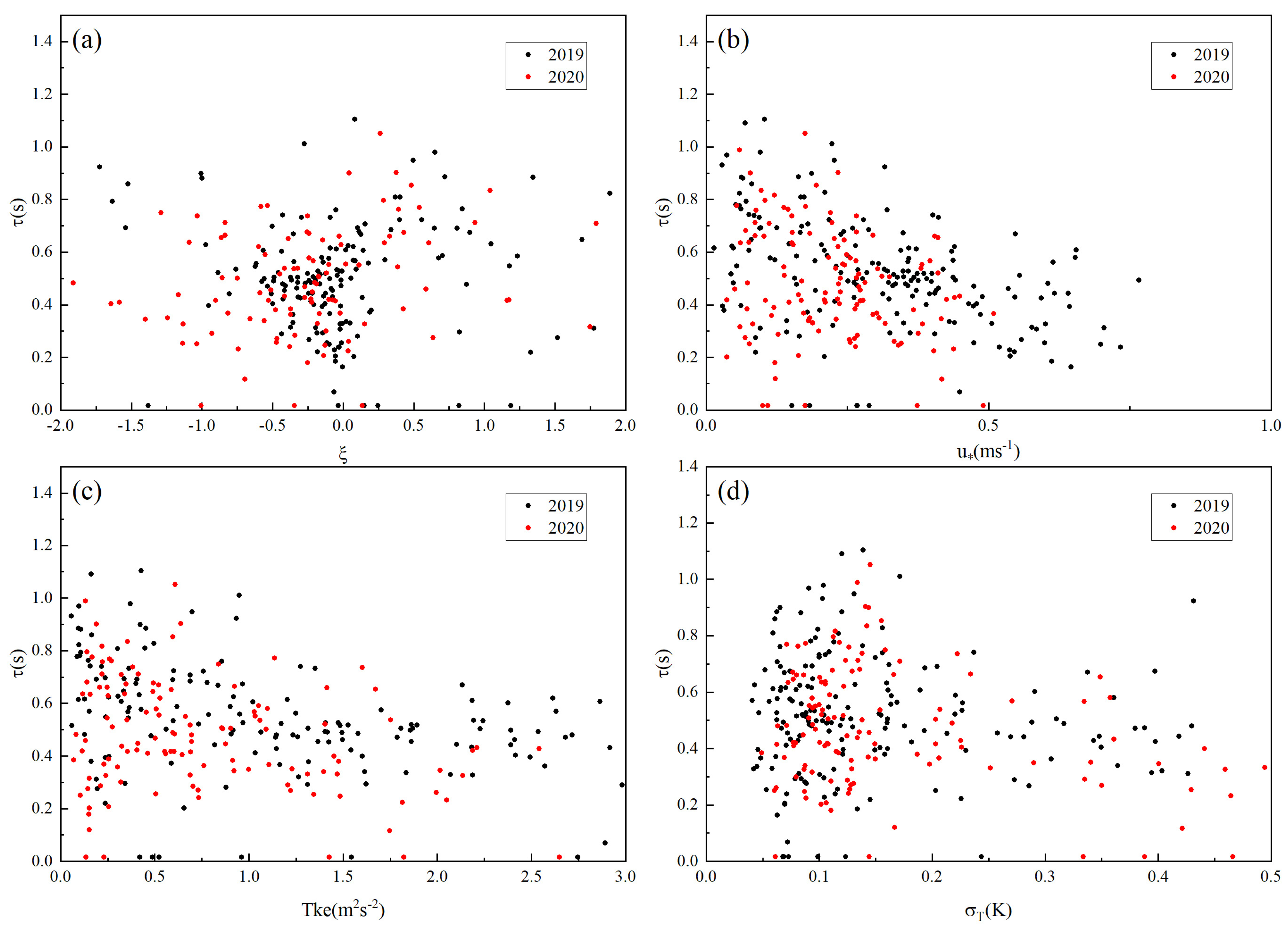
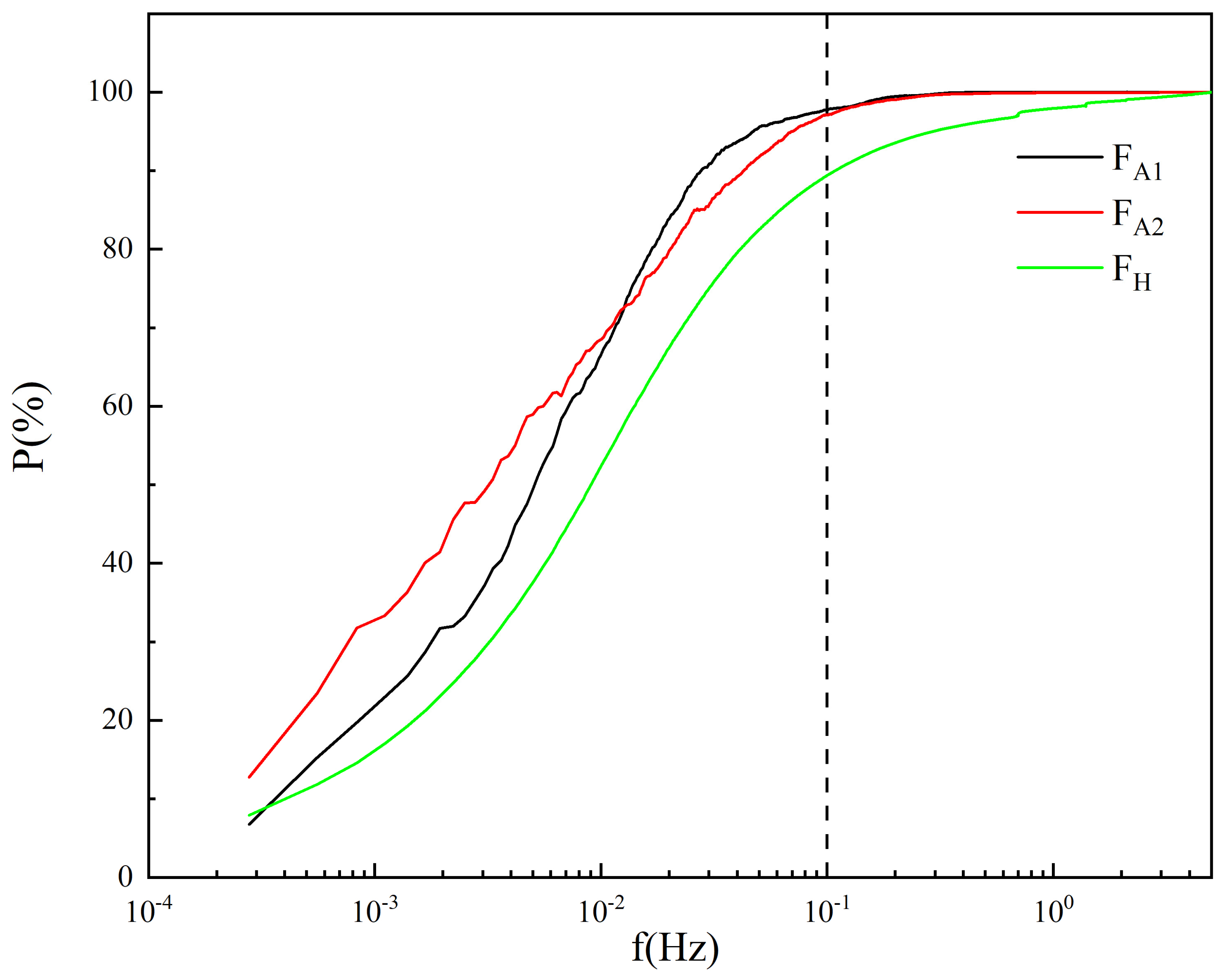
3.1. Characteristics of Aerosol Number Concentration Spectrum

First, the power spectrum characteristics of the concentration fluctuation of the aerosol instance number are given. The measurement times in Figure 1 are 12:00 on 20 January 2019 (a), 15:00 on 23 January 2019 (b), and 16:00 on 29 March 2019 (c). The measurement time of Figure 1d was measured for two adjacent hours, from 14:46 on 19 April 2021 to 16:56 on 19 April 2021, including ten minutes of replacement of the intake pipe. According to the degree of high-frequency attenuation, aerosol power spectral density can be divided into two categories, as shown in Figure 1a,b, which are strong attenuation and almost no attenuation, respectively. Among them, the aerosol number concentration power spectrum with strong attenuation satisfies the ‘−5/3’ law in the low-frequency part of the inertia subregion, and the higher-frequency part has obvious attenuation, accounting for approximately 93.1%; the power spectrum with almost no attenuation satisfies the ‘−5/3’ law well in the inertia subregion. The aerosol number concentration power spectrum with strong attenuation can be divided into four parts, as shown in Figure 1a: the outer scale region, the low-frequency part of the inertial subregion, the high-frequency part of the inertial subregion, and the noise region. The dividing point between the outer scale region A1 and the inertial subregion can be determined by the peak value of the power spectrum, and the cutoff point between the inertial subregion and the noise region is the noise point, which is usually determined by the very low value of the high-frequency range. The inertia subregion can be divided into two parts, A2 and A3. In the lower-frequency A2 region, its power spectral density conforms to the “−5/3” law, and in the higher-frequency A3 region, its slope is significantly less than −2/3, that is, the spectral density in this part is low. In the inertia subregion, it is difficult to determine the boundary point between the A2 part and the A3 part. It can be seen from the description of the transfer function that the attenuation amplitude gradually increases, and the A2 part also has a small degree of attenuation. A rough dividing point is given in the figure as a reference.
When measuring on the ground, the air intake pipe is not connected, and the aerosol number concentration power spectrum is shown in Figure 1c, which satisfies the “−5/3” law well in the inertial subregion, and there are some noise signals in the high-frequency part. The black line in Figure 1d is the power spectrum of the unconnected intake pipe when measured on the ground, and the red line is the power spectrum of the connected intake pipe. As seen from the figure, when the intake duct is connected, the high-frequency part has obvious attenuation.
Figure 1a shows the main type of aerosol power spectrum in the flux measurement. The main difference between it and the usual three-dimensional wind speed, temperature, and aerosol concentration fluctuation power spectrum shown in Figure 1c is that the ground is not connected to the air intake pipe. The noise signal is pronounced and attenuated in the high-frequency part of the inertial subregion. Figure 1d shows the power spectra of the aerosol concentration fluctuations in two adjacent time periods, indicating that these attenuations are mainly caused by the intake duct, which is similar to the water vapor concentration fluctuations when the water vapor flux is measured using the closed-circuit eddy correlation method.
In experiments 1 and 3, the instrument was placed in a box on the iron tower, the air was drawn into the instrument through the intake pipe to measure the aerosol concentration in the air, and its spectrum was significantly attenuated at high frequencies. In experiment 2, when the instrument was installed on the ground for measurement, most of the high-frequency part of the aerosol power spectrum did not show obvious attenuation.
Figure 2 shows an example of calculating the characteristic time of the aerosol concentration fluctuation power spectrum using the method in Section 2.3. The standard spectrum in this paper is shown by the green line in Figure 2a, which is the standard “−5/3” line, the black line is the normalized aerosol concentration fluctuation power spectrum, and the red line is the normalized and corrected aerosol concentration fluctuation power spectrum E m f T f f 1 f 2 E m f T f d f . As mentioned in Section 2.3, the upper and lower limits of the correction interval are taken as 0.0060 Hz and 0.9469 Hz, respectively, and different τ values are taken to obtain different errors ∆R. The f 0 when ΔR takes the minimum value corresponds to the correct feature time.
Figure 3 shows that the characteristic time of the aerosol fluctuation power spectrum is not fixed; that is, its transfer function is not uniquely determined by the measuring instrument system. Atmospheric turbulent motion and the fluctuating characteristics of the aerosol itself are factors that may affect its characteristic time.
Figure 4 shows the relationship between the characteristic time and some atmospheric parameters, which are atmospheric stability ξ, friction velocity u * , turbulent kinetic energy TKE, and temperature variance δ.
ξ = z L
L = u * 3 k g w θ ¯ θ ¯
u * = u w ¯ 2 + v w ¯ 2 1 4
TKE = u 2 + v 2 + w 2 1 2 ¯
where z is the height of the observation point above the canopy, the two experiments are 21 m and 18 m, respectively, k is the Karman constant, k = 0.4, g is the acceleration of gravity, g = 9.8 m/s2, u, v and w are the three-dimensional wind speeds, θ is the potential temperature,’represents the fluctuation, and—represents the mean value.
Figure 4b shows that the characteristic time of the aerosol concentration fluctuation power spectrum is affected by friction velocity u * . As the friction velocity increases, the characteristic time decreases. In Figure 4a,c,d, the effect of turbulence parameters is not very significant.
In the experimental results of this paper, noise signals generally exist in the high-frequency range, and the mean value of the spectral density of 3 Hz to 5 Hz in the fluctuating power spectrum of aerosol concentration is taken as the intensity of the noise. Figure 5a shows that the intensity of the noise increases with increasing standard deviation. Taking the integral of the noise intensity in the power spectrum interval, the total energy of the noise can be obtained, and then the proportion of the noise energy in the variance can be obtained. Figure 5b shows that the energy proportion of the noise increases as the standard deviation (variance) increases and decreases. This in turn leads to an increase in the minimum frequency at which the noise signal can be observed in the power spectrum as the standard deviation (variance) increases. That is, as shown in Figure 5d, when the variance is small, the high-frequency attenuation signal is more likely to be covered by noise, and the obtained characteristic time is also smaller. When the variance is larger, the calculated characteristic time is also larger. When the variance is larger, noise appears more frequently. The attenuation is more obvious.

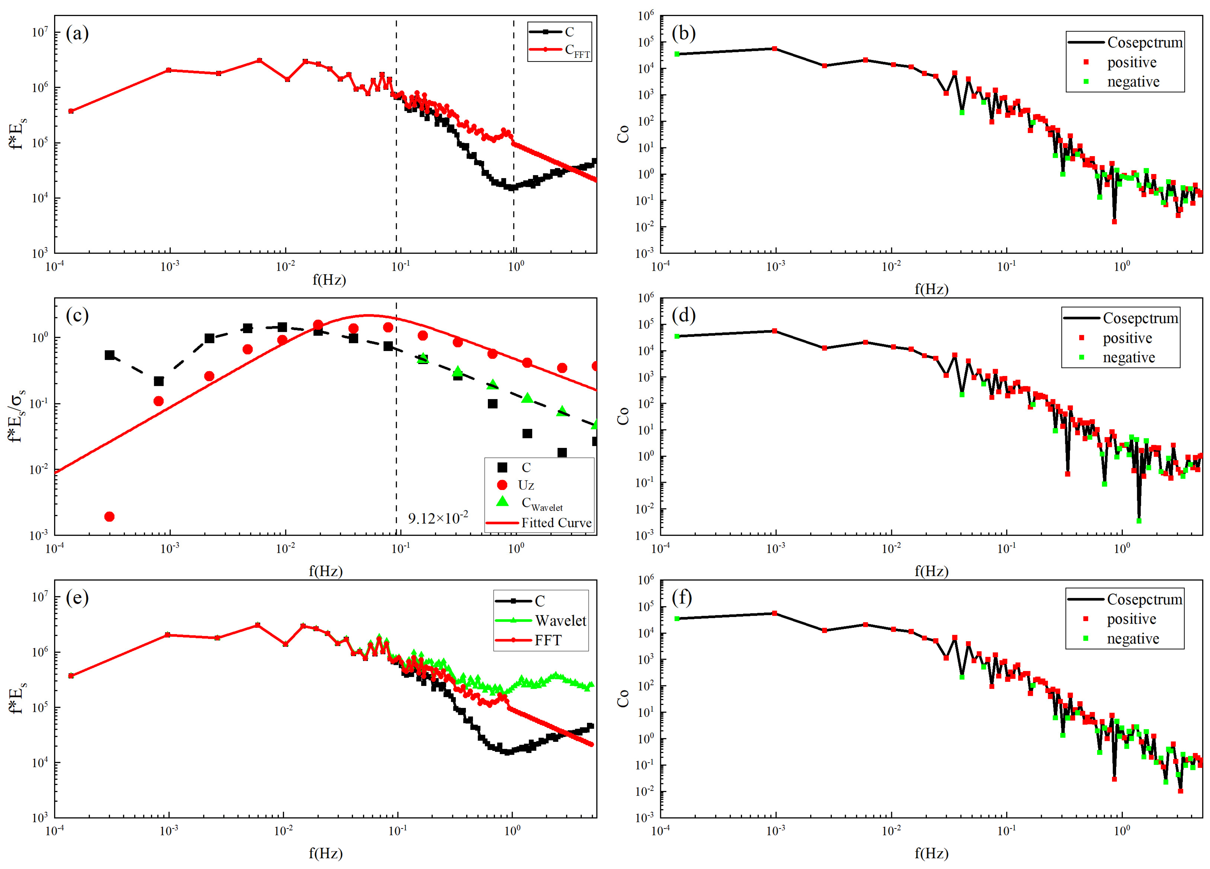
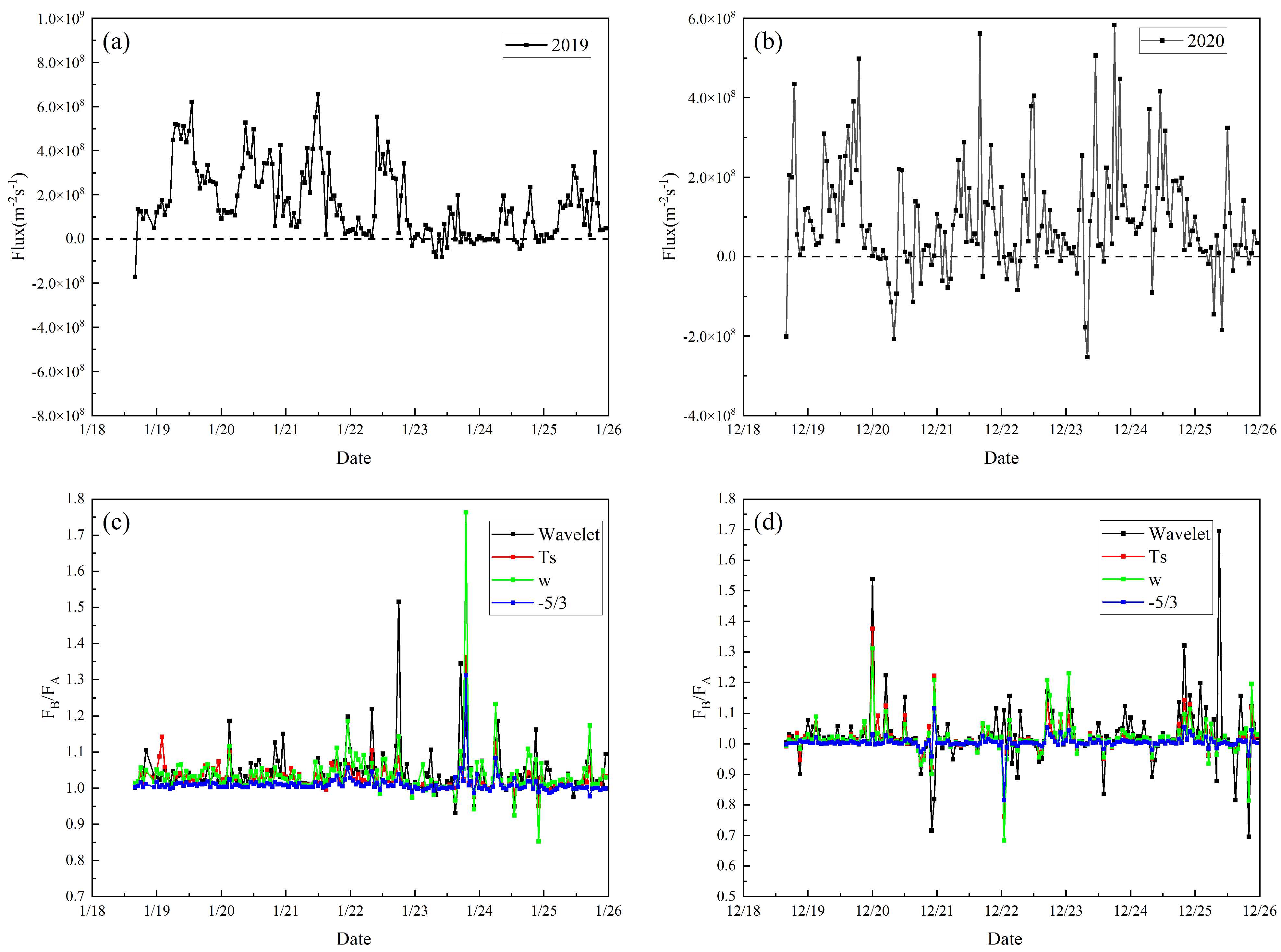
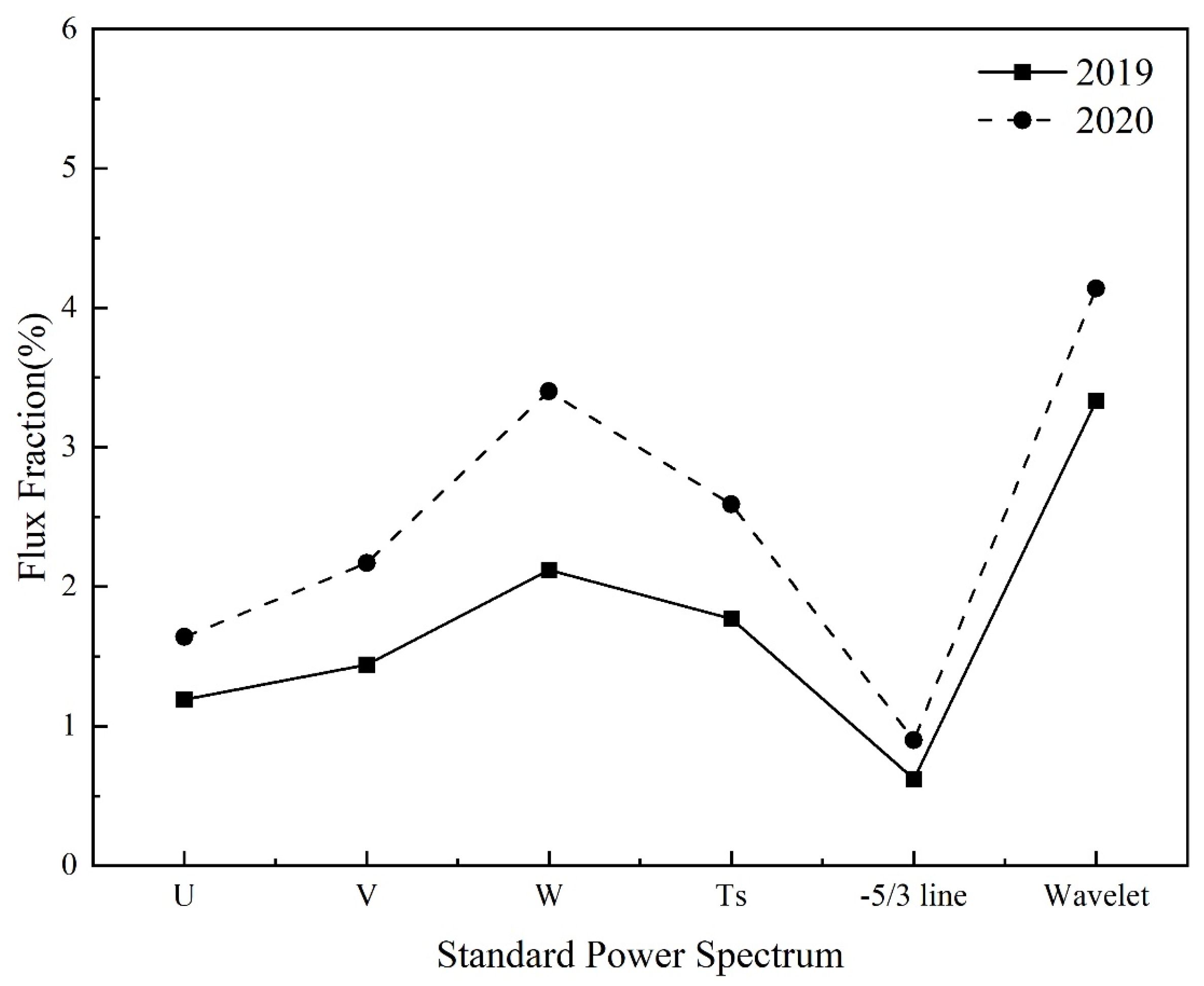
3.2. The Results of Two Correction Methods for High-Frequency Attenuation Correction and the Influence on Flux Measurement

The observed aerosol number concentration spectrum was corrected by the FFT-based method and the wavelet-based method, and the corrected aerosol number concentration fluctuation was obtained. As shown in Figure 6, in this example, both methods can effectively compensate for high-frequency energy loss. The advantage of the wavelet method is that it can correct different phase angles at the same frequency. The disadvantage is that compared with the FFT method, there are only 15 frequencies in a one-hour time period, and the resolution in the frequency domain is lower.
Figure 7 presents the aerosol fluxes during the observation period and the correction ratios obtained by different correction methods. For the same standard spectrum, the correction ratio for part of the time is relatively large, reaching more than 20%. This is because the absolute value of the flux in these time periods is small, and the flux contribution of each frequency is almost equal to positive and negative. In the high-frequency part, small changes can change large proportions. Figure 8 shows the average correction ratio for different correction schemes. As shown in Figure 8, the high-frequency correction based on wavelet transform will have an impact of approximately 4% on the aerosol flux results. The magnitude of the high-frequency correction based on FFT depends on the standard spectrum obtained at the characteristic time. When the standard spectrum is vertical and the power spectrum of the wind speed w is used, the correction amplitude is the largest, approximately 4%. When the “−5/3” power law line is selected for the standard spectrum, the correction amplitude is the smallest, approximately 1%. The results obtained from different standard spectra are between 1–4%.
If the corrected aerosol concentration is regarded as the true aerosol concentration in the atmosphere, the high-frequency attenuation of the measured aerosol number concentration power spectrum will cause a 1–4% error in the flux measurement. The aerosol flux is equal to the integral of the cross-power spectrum of aerosol concentration and vertical velocity over frequency. In the high-frequency part, the cross-power spectrum has positive and negative values. When the Fourier transformed spectrum is directly corrected, the magnitude of the correction will affect the value of the cross-power spectrum without changing its positive or negative value. The wavelet transform can change the positive and negative values of the cross-power spectrum by adjusting the wavelet coefficients on different position factors at the same frequency, which cannot be achieved by the FFT correction. In addition, not all the aerosol fluxes in the time period will increase after correction. This is because in the cross-power spectrum of aerosol fluxes, the high-frequency part has positive and negative parts, and the correction of the aerosol concentration data will increase the absolute value of the high-frequency cross-power spectral energy. The influence on the integration of the cross-power spectrum truly depends on whether the positive or negative of the corresponding frequency is the same as the total positive and negative.
The cross-power spectrum of aerosol number concentration and vertical wind speed is the distribution of the aerosol number concentration flux at different frequencies. Figure 9 shows the cumulative proportion of sensible heat flux and aerosol number concentration flux contributions below different frequencies. The three curves represent the two aerosol flux experiments and the long-term sensible heat flux. The sensible heat flux is not attenuated at high frequencies, while the aerosol flux is attenuated at high frequencies. The figure shows that approximately 90% of the sensible heat flux is contributed by fluctuations with frequencies less than 0.1 Hz, and this proportion rises to 98% for the measured aerosol flux, which is mainly because the proportion of aerosol flux after high-frequency attenuation is lower than that of unattenuated aerosol flux. Taking the sensible heat flux as the reference for the high-frequency aerosol flux that is not attenuated, the aerosol flux above 0.1 Hz accounts for approximately 10%.

4. Conclusions and Discussion

In this paper, two aerosol flux observation experiments were carried out in the near-surface layer, and a long-term observation experiment was carried out on the surface. The observed data show that the aerosol concentration fluctuation spectrum in the near-surface layer conforms to the “−5/3” law in the inertial subregion, and the aerosol concentration fluctuation conforms to the turbulent motion characteristics. In the actual flux measurement, due to the attenuation of the intake duct, the aerosol number concentration power spectrum will have a significant attenuation at high frequencies, thus deviating from the “−5/3” law of the setup.
The response function obtained from the transmission theory is a function of the characteristic time τ of the instrument. By fitting the experimental data, the characteristic time of the measurement system in this experiment, the characteristic time of the aerosol concentration fluctuation spectrum under the same measurement conditions, and the mean and standard deviation of the aerosol concentration are obtained. It is almost irrelevant to atmospheric turbulence characteristic quantities. Therefore, the strength of the attenuation of the intake duct is mainly affected by the characteristics of the aerosol itself and is not affected by atmospheric turbulence.
In this paper, two methods are used to correct the measured aerosol flux. The correction results show that the correction of the high frequency of the aerosol power spectrum will have an impact of approximately 1–4% on the aerosol flux; that is, the results obtained from the observational experiments are close to the real results. In the observations carried out in Helsinki and Cabauw, the attenuation ratio of the aerosol flux obtained by various methods varies from 4% to 35% [22]. Compared with the previous measurement results, this paper adopts the shorter length of the intake duct and the smaller inner diameter, the shorter the characteristic time, and the smaller error of the obtained aerosol number concentration flux. Therefore, in the observation, the aerosol concentration measuring instrument is installed as close as possible to the ultrasonic anemometer, which is beneficial to reduce the observation error. On the other hand, due to the large size of the aerosol particle counter, too-short inlet tubes can cause the flow field to be affected by the instrument itself. The length of the sampling tube must be carefully considered.
When correcting the flux using the wavelet-based method, the cutoff frequency and the correction amplitude will affect the final flux correction ratio, but the approximate correction amplitude is not significantly different. Further research is needed to determine which method is more accurate for obtaining unattenuated aerosol fluxes.
Under the isotropic assumption, the power law of the cross-power spectrum satisfies the “−7/3” law [23], the flux is the integral of the cross-power spectrum, and the contribution of low frequencies is much greater than that of high frequencies. The data analysis of sensible heat flux shows that the cross-power spectrum of temperature and vertical velocity greater than 0.1 Hz accounts for approximately 10% of the total flux. Similarly, the attenuation effect of the high-frequency portion of the cross-power spectrum of aerosol number concentration and vertical velocity is small with respect to the total flux. In the measured aerosol number concentration flux, the effect of high-frequency attenuation gradually increases with increasing characteristic time. Therefore, the characteristic time in the measurement of aerosol flux needs to be controlled within an acceptable range. Reducing the length of the intake pipe and increasing the flow rate of the pumped air are highly effective methods to reduce the characteristic time.

Supplementary Materials

The following supporting information can be downloaded at: https://www.mdpi.com/article/10.3390/atmos16030332/s1, Figure S1. The 4-story building and 18 m tower; Figure S2. The tower with three ultrasonic anemometers and five levels of RM Young 03002 anemometers and HMP155A temperature and humidity sensors. During experiment #3, a TSI3788 water-based condensate particle counter was installed in a sealed box fixed on the iron tower as indicated by the arrows; Figure S3. Test experiments on the rooftop; Figure S4. An example of data processing at 14:00–15:00 on 20 January 2019. Figure 1a is the original data, and there are some zeros around the 15000th point. That is because every two hours of data are stored in a file, and about 2 seconds of data are lost during file storage. Then, we calculate the different ∆x between two adjacent points as shown in Figure 1b. Figure 1c is the histogram of ∆x, and the standard deviation of ∆x is 336.72. The ∆x around the zeros is too large and not shown in the figure. The values are all multiples of 100 because of the resolution of the instrument. So, only the zeros will be removed in this case. Figure S5d is the power spectrum of original data and processed data; Figure S5. Data processing at 13:00–14:00 on 20 January 2019. The standard deviation of ∆x is 315.95. No point is removed in this case. Figure S5d is the power spectrum of original data and processed data. Unless the differences are particularly large, this approach generally does not strip out useful data.

Author Contributions

Conceptualization, H.L.; methodology, H.L.; software, H.L. and R.Y.; formal analysis, H.L.; investigation, Q.Z. and X.Z.; data curation, B.Z.; writing—original draft, H.L.; writing—review and editing, Y.L. (Yuan Liu) and Y.L. (Yongchang Li). All authors have read and agreed to the published version of the manuscript.

Funding

This research was funded by The National Natural Science Foundation of China, grant number (42105076, 42075131, 42475085); University Natural Science Research Project of Anhui Province [grant number 2024AH050265]; China Meteorologica1Administration Xiong’an Atmospheric Boundary Layer Key Laboratory [2023LABL-B22]; general projects of Anhui Jianzhu University [2022QDZ20]; The Natural Science Foundation of Anhui Province (2208085UQ01); Anhui Provincial Meteorological Detection Equipment Engineering Technology Research Center Open Fund (2023QXTC08).

Institutional Review Board Statement

Not applicable.

Informed Consent Statement

Not applicable.

Data Availability Statement

The original contributions presented in this study are included in the article/Supplementary Materials. Further inquiries can be directed to the corresponding author(s).

Conflicts of Interest

The authors declare no conflicts of interest.

References

  1. Huang, R.-J.; Zhang, Y.; Bozzetti, C.; Ho, K.-F.; Cao, J.-J.; Han, Y.; Daellenbach, K.R.; Slowik, J.G.; Platt, S.M.; Canonaco, F.; et al. High secondary aerosol contribution to particulate pollution during haze events in China. Nature 2014, 514, 218–222. [Google Scholar] [CrossRef] [PubMed]
  2. Mahowald, N.; Ward, D.S.; Kloster, S.; Flanner, M.G.; Heald, C.L.; Heavens, N.G.; Hess, P.G.; Lamarque, J.F.; Chuang, P.Y. Aerosol Impacts on Climate and Biogeochemistry. Annu. Rev. Environ. Resour. 2011, 36, 45–74. [Google Scholar] [CrossRef]
  3. Kobayashi, H.; Hayashi, M.; Shiraishi, K.; Nakura, Y.; Enomoto, T.; Miura, K.; Takahashi, H.; Igarashi, Y.; Naoe, H.; Kaneyasu, N.; et al. Development of a polarization optical particle counter capable of aerosol type classification. Atmos. Environ. 2014, 97, 486–492. [Google Scholar] [CrossRef]
  4. Qin, J.; Tang, W.; Yang, K.; Lu, N.; Niu, X.; Liang, S. An efficient physically based parameterization to derive surface solar irradiance based on satellite atmospheric products. J. Geophys. Res. Atmos. 2015, 120, 4975–4988. [Google Scholar] [CrossRef]
  5. Li, Y.; Cai, X.; Li, M.; Jiang, Z.; Tang, F.; Zhang, S.; Shui, T.; Zhu, S. Review of the Urban Carbon Flux and Energy Balance Based on the Eddy Covariance Technique. Aerosol Air Qual. Res. 2024, 24, 230245. [Google Scholar] [CrossRef]
  6. Yuan, R.; Luo, T.; Sun, J.; Liu, H.; Fu, Y.; Wang, Z. A new method for estimating aerosol mass flux in the urban surface layer using LAS technology. Atmos. Meas. Tech. 2016, 9, 1925–1937. [Google Scholar] [CrossRef]
  7. Yuan, R.; Luo, T.; Sun, J.; Zeng, Z.; Ge, C.; Fu, Y. A new method for measuring the imaginary part of the atmospheric refractive index structure parameter in the urban surface layer. Atmos. Meas. Tech. Phys. 2015, 15, 2521–2531. [Google Scholar] [CrossRef]
  8. Hill, R.J. Spectra of fluctuations in refractivity, temperature, humidity, and the temperature-humidity cospectrum in the inertial and dissipation ranges. Radio Sci. 1978, 13, 953–961. [Google Scholar] [CrossRef]
  9. Batchelor, G.K. Kolmogoroff’s theory of locally isotropic turbulence. In Mathematical Proceedings of the Cambridge Philosophical Society; Cambridge University Press: Cambridge, UK, 1947; Volume 43, pp. 533–559. [Google Scholar]
  10. Tiwari, S.; Srivastava, A.; Bisht, D.; Parmita, P.; Srivastava, M.K.; Attri, S. Diurnal and seasonal variations of black carbon and PM2.5 over New Delhi, India: Influence of meteorology. Atmos. Res. 2013, 125–126, 50–62. [Google Scholar] [CrossRef]
  11. Jokinen, T.; Kontkanen, J.; Lehtipalo, K.; Manninen, H.E.; Aalto, J.; Porcar-Castell, A.; Garmash, O.; Nieminen, T.; Ehn, M.; Kangasluoma, J.; et al. Solar eclipse demonstrating the importance of photochemistry in new particle formation. Sci. Rep. 2017, 7, srep45707. [Google Scholar] [CrossRef]
  12. Ahlm, L.; Krejci, R.; Nilsson, E.D.; Mårtensson, E.M.; Vogt, M.; Artaxo, P. Emission and dry deposition of accumulation mode particles in the Amazon Basin. Atmos. Meas. Tech. 2010, 10, 10237–10253. [Google Scholar] [CrossRef]
  13. Vogt, M.; Nilsson, E.D.; Ahlm, L.; MÕrtensson, E.M.; Johansson, C. Seasonal and diurnal cycles of 0.25–2.5 mu m aerosol fluxes over urban Stockholm, Sweden. Tellus Ser. B Chem. Phys. Meteorol. 2011, 63, 935–951. [Google Scholar] [CrossRef]
  14. Aslan, T.; Peltola, O.; Ibrom, A.; Nemitz, E.; Rannik, Ü.; Mammarella, I. The high-frequency response correction of eddy covariance fluxes—Part 2: An experimental approach for analysing noisy measurements of small fluxes. Atmos. Meas. Tech. 2021, 14, 5089–5106. [Google Scholar] [CrossRef]
  15. Massman, W. A simple method for estimating frequency response corrections for eddy covariance systems. Agric. For. Meteorol. 2000, 104, 185–198. [Google Scholar] [CrossRef]
  16. Ripamonti, G.; Järvi, L.; Mølgaard, B.; Hussein, T.; Nordbo, A.; Hämeri, K. The effect of local sources on aerosol particle number size distribution, concentrations and fluxes in Helsinki, Finland. Tellus B Chem. Phys. Meteorol. 2013, 65, 19786. [Google Scholar] [CrossRef]
  17. Horst, T.W. A simple formula for attenuation of eddy fluxes measured with first-order-response scalar sensors. Bound. Layer Meteorol. 1997, 82, 219–233. [Google Scholar] [CrossRef]
  18. De Ligne, A.; Heinesch, B.; Aubinet, M. New Transfer Functions for Correcting Turbulent Water Vapour Fluxes. Bound. Layer Meteorol. 2010, 137, 205–221. [Google Scholar] [CrossRef]
  19. Ibrom, A.; Dellwik, E.; Flyvbjerg, H.; Jensen, N.O.; Pilegaard, K. Strong low-pass filtering effects on water vapour flux measurements with closed-path eddy correlation systems. Agric. For. Meteorol. 2007, 147, 140–156. [Google Scholar] [CrossRef]
  20. Nordbo, A.; Katul, G. A Wavelet-Based Correction Method for Eddy-Covariance High-Frequency Losses in Scalar Concentration Measurements. Bound. Layer Meteorol. 2012, 146, 81–102. [Google Scholar] [CrossRef]
  21. Enroth, J.; Kangasluoma, J.; Korhonen, F.; Hering, S.; Picard, D.; Lewis, G.; Attoui, M.; Petäjä, T. On the time response determination of condensation particle counters. Aerosol Sci. Technol. 2018, 52, 778–787. [Google Scholar] [CrossRef]
  22. Oosterwijk, A.; Henzing, B.; Järvi, L. On the application of spectral corrections to particle flux measurements. Environ. Sci. Nano 2018, 5, 2315–2324. [Google Scholar] [CrossRef]
  23. Cheng, Y.; Li, Q.; Grachev, A.; Argentini, S.; Fernando, H.J.S.; Gentine, P. Power-Law Scaling of Turbulence Cospectra for the Stably Stratified Atmospheric Boundary Layer. Bound. Layer Meteorol. 2020, 177, 1–18. [Google Scholar] [CrossRef]
Figure 1. Four typical examples of a normalized aerosol number concentration spectrum (ad); the black line is the aerosol number concentration power spectrum, the red dot line is the “−2/3” line, and the green dashed line in (a) divides the power spectrum into 4 parts. The abscissa is the frequency, and the ordinate is the power spectral density multiplied by the frequency divided by the variance. Therefore, the noise is the “+1” slope in high frequency.
Atmosphere 16 00332 g001
Figure 2. (a) shows the aerosol power spectrum before correction (black line) and the modified aerosol power spectrum (red line), the green line is the standard “−5/3” line, the vertical dashed line represents the upper and lower limits of the fitting interval (0.0060 Hz and 0.9469 Hz), the black line of this interval is corrected to the red line by the transfer function, the power spectrum is normalized by integration, and the error of the red line and green line is calculated. (b) is the error corresponding to different f 0 , and the frequency with the smallest error corresponds to the correct feature time.
Atmosphere 16 00332 g002
Figure 3. The characteristic time obtained when the standard ‘−5/3’ lines are used as standard spectra. Figure (a) is experiments in 2019, and (b) is experiments in 2020.
Atmosphere 16 00332 g003
Figure 4. Scatterplot of characteristic time and partial atmospheric turbulence parameters, where (a) is stability, (b) is friction velocity, (c) is turbulent flow energy, and (d) is temperature standard deviation.
Atmosphere 16 00332 g004
Figure 5. Distribution of characteristic time. Figure (a) is the relationship between noise spectral density and standard deviation, Figure (b) is the relationship between the energy proportion of noise and standard deviation, Figure (c) is the relationship between frequency and the standard deviation of noise, and Figure (d) is the relationship between characteristic time (with the −5/3 line as standard) and standard deviation.
Atmosphere 16 00332 g005
Figure 6. Examples of a high-frequency correction of the power spectrum. (a) is an FFT correction example, the black line is the power spectrum of the measured data, and the red line is the corrected power spectrum; (c) is an example of the wavelet method, the red dot is the wavelet spectrum of vertical speed, the black dot is the wavelet spectrum of aerosol concentration, and the black dotted line is the corrected wavelet spectrum; (e) is the comparison of the correction effect of the two methods; (b,d,f) are the cross-power spectrum of measured data, FFT correction, and wavelet correction, the red dot is positive, indicating upward flux contribution, and the green dot is negative, indicating downward flux contribution.
Atmosphere 16 00332 g006
Figure 7. Aerosol number concentration flux before spectral correction (a,b) and ratio of flux correction (c,d).
Atmosphere 16 00332 g007
Figure 8. Flux ratio modified by different correction methods.
Atmosphere 16 00332 g008
Figure 9. Cumulative contribution of sensible heat flux and aerosol number concentration flux at different frequencies (black and red lines are two aerosol flux observation experiments, respectively, and the green line is the average of sensible heat flux observed throughout 2018).
Atmosphere 16 00332 g009
Table 1. Experimental setup.
Experiment No.TimeSiteIntake PipeThe Time Spent by the Air Sample to Go Through the Sampling LineReynolds NumberFlow Rate
118 January 2019–27 February 2019On the tower, 18 m from the bottom of the tower2 m stainless-steel intake pipe and 1 m hose, inner diameter of 4 mm1.51 s5401.5 L/min
211 March 2019–1 April 20191 m from the bottom of the towerNone 1.5 L/min
318 December 2020–26 December 2020On the tower, 15 m from the bottom of the tower2 m stainless-steel intake pipe and 1 m hose, inner diameter of 4 mm1.51 s5401.5 L/min
Disclaimer/Publisher’s Note: The statements, opinions and data contained in all publications are solely those of the individual author(s) and contributor(s) and not of MDPI and/or the editor(s). MDPI and/or the editor(s) disclaim responsibility for any injury to people or property resulting from any ideas, methods, instructions or products referred to in the content.

