The Role of Atmospheric Circulation Patterns in Water Storage of the World’s Largest High-Altitude Landslide-Dammed Lake

Abstract

This study reconstructed the annual lake surface area (LSA) and absolute lake water storage (LWS) changes of Lake Sarez, the world’s largest high-altitude landslide-dammed lake, from 1992 to 2023 using multi-source remote sensing data. All available Landsat images were used to extract the LSA using an improved multi-index threshold method, which incorporates a slope mask and threshold adjustment to enhance the boundary delineation accuracy (Kappa coefficient = 0.94). By combining the LSA with high-resolution DEM and the GLOBathy bathymetry dataset, the absolute LWS was reconstructed, fluctuating between 12.3 × 10⁹ and 12.8 × 10⁹ m³. A water balance analysis revealed that inflow runoff (IRO) was the primary driver of LWS changes, contributing 54.57%. The cross-wavelet transform and wavelet coherence analyses showed that the precipitation (PRE) and snow water equivalent (SWE) were key climatic factors that directly influenced the variability of IRO, impacting the interannual water availability in the lake, with PRE having a more sustained impact. Temperature indirectly regulated IRO by affecting SWE and potential evapotranspiration. Furthermore, IRO exhibited different resonance periods and time lags with various atmospheric circulation factors, with the Pacific Decadal Oscillation and North Atlantic Oscillation having the most significant influence on its interannual variations. These findings provide crucial insights into the hydrological behavior of Lake Sarez under climate change and offer a novel approach for studying water storage dynamics in high-altitude landslide-dammed lakes, thereby supporting regional water resource management and ecological conservation.

1. Introduction

Lakes serve as crucial components of the hydrological cycle and play a vital role in human well-being and ecological systems [1,2]. However, understanding the complex responses of lakes to climate change and anthropogenic activities remains a challenging scientific issue in international research [3,4,5]. This challenge is especially evident in arid and semi-arid regions, such as Central Asia [6,7]. Central Asia ranks among the regions with one of the highest numbers of inland lakes globally, with over 3000 lakes exceeding 1 km² [8]. These lakes in Central Asia are crucial for supplying water to arid regions and are sensitive to environmental changes, making them valuable indicators of climate change [9,10]. High-altitude lakes in Central Asia, in particular, exhibit less anthropogenic influence and, thus, display a heightened sensitivity to climate change compared to their low-altitude counterparts [11]. The importance of these high-altitude lakes extends beyond Central Asia, as similar lakes around the world, such as those in the Tibetan Plateau [12], Pyrenees [13], and Andes [14], are also highly sensitive to environmental changes. Located in remote and ecologically sensitive regions, these lakes offer valuable insights into global climate patterns. Research on high-altitude lakes in Central Asia provides an important link to understanding the impacts of climate change on similar ecosystems worldwide. Such studies are vital for managing water resources in both the local and global contexts. Revealing the dynamic fluctuations of these lakes and elucidating their driving forces can significantly advance our understanding of global and regional climate change and its subsequent impacts on ecosystems.

Lake water storage (LWS) is a fundamental response to climate change [15,16], providing a more comprehensive reflection of climate impacts than the lake surface area (LSA) and lake water level (LWL) [12,17]. However, the existing research on high-altitude lakes in Central Asia has predominantly focused on changes in the LSA or LWL owing to insufficient monitoring data, resulting in limitations in accuracy and temporal continuity [18,19,20]. Despite the use of remote sensing techniques to reconstruct relative long-term water level variations for specific high-altitude lakes in Central Asia [21,22], there is a dearth of analysis regarding the climatic drivers underlying these changes, and the absolute LWS remains poorly understood because of the lack of bathymetric data. These limitations impede a comprehensive understanding of high-altitude lakes in Central Asia, necessitating the urgent development of a method capable of rapidly and accurately measuring the absolute LWS and its variations. Traditional measurement methods rely on shipborne depth sounders to measure the depth of water at specific points and interpolate them to generate bathymetric maps to calculate the lake volumes [23]. Although precise, this approach is labor-intensive and challenging to implement at high altitudes in Central Asia, where infrastructure and human resources are lacking. With the progress made in remote sensing techniques coupled with the use of geographic information systems and geophysical models, it has become feasible to effectively and economically simulate lake bathymetry [24,25]. For example, the GLOBathy dataset utilizes these technologies to estimate the lake depth, providing a viable approach for studying lakes in regions with limited data availability [25]. However, bathymetric data are typically based on measurements taken at specific periods, reflecting the lake’s depth and water storage at specific points in time. In cases of LWS changes, especially when the water level surpasses the recorded depths from bathymetric surveys, it is necessary to integrate the extracted LSA with digital elevation models (DEMs) or satellite altimetry data to assess the relative LWS changes above bathymetric data [26].

The Pamir Plateau in Central Asia harbors numerous high-altitude lakes, including more than 100 landslide-dammed lakes [27]. Their hydrological dynamics are highly dependent on regional climatic conditions, and, because of their remote location, these lakes are especially sensitive to changes in climate [19,28]. Lake Sarez, the world’s largest and deepest high-altitude landslide-dammed lake located on the Pamir Plateau in Central Asia [29], is a representative example of the landslide-dammed lakes in the region. Because of its high altitude and minimal human influence, it is an ideal site for studying hydrological changes in high-altitude lakes across Central Asia. Furthermore, Lake Sarez is considered a major global natural disaster risk [30,31]. Understanding LWS changes in Lake Sarez can provide new insights into how these lakes in the Pamir Plateau respond to climate change, and is crucial for water resource management and regional security. Formed in 1911, when a massive landslide blocked a river after it was triggered by a powerful earthquake, Lake Sarez now has a maximum depth exceeding 500 m [32]. Lake Sarez poses significant risks and has been listed among the world’s top ten potentially deadly natural disasters owing to the possibility of dam failure [30]. Monitoring long-term hydrological changes in Lake Sarez is important for water security assessment and management. Extensive studies have focused on disaster risk assessment and dam stability monitoring [31,33,34,35,36]. However, research on long-term hydrological changes in Lake Sarez, particularly with regard to the absolute LWS and the underlying driving factors, remains limited. This gap restricts our understanding of high-altitude lake dynamics in Central Asia, and hinders the development of effective management strategies for landslide-dammed lakes with high potential hazards.

Based on the aforementioned understanding and research gaps, the aims of this study were as follows: (1) to generate an annual LSA using all available Landsat images and, in conjunction with bathymetric data and high-resolution DEM, to construct a precise interannual series of absolute LWS changes in Lake Sarez from 1992 to 2023 and analyze its temporal evolution characteristics, providing a more comprehensive understanding of long-term LWS variations; and (2) to employ a water balance model and wavelet analysis to comprehensively investigate and analyze the driving factors behind the absolute LWS changes in Lake Sarez and their underlying mechanisms, contributing to improved disaster risk management and regional water resource strategies.

2. Materials and Methods

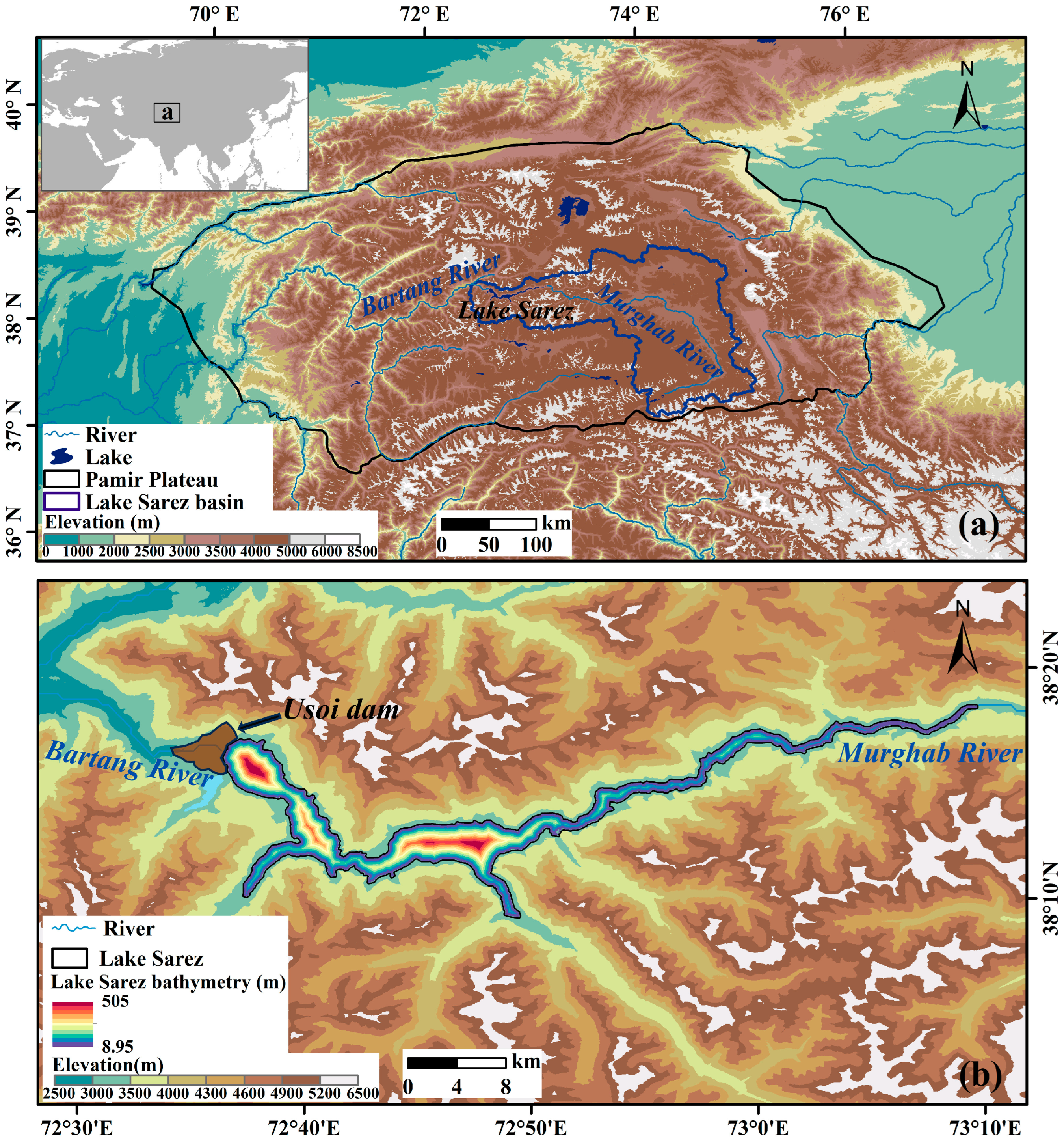
2.1. Geographical Settings

On 18 February 1911, a seismic event of significant magnitude, estimated at a Richter scale of 7.7 [31], occurred in the Pamir region, causing a massive landslide that formed the 560-meters-high Usoi Dam. This natural dam blocked the Murghab River Valley, ultimately creating Lake Sarez, the world’s largest and deepest high-altitude landslide-dammed lake [32] (Figure 1). The lake watershed, characterized by rugged terrain and minimal human presence, exhibits an average elevation of 3264 m. The lake extends approximately 55.8 km in length, with an average width of 1.44 km, a maximum depth over 500 m, a surface area around 84.37 km², and a catchment area totaling 19,564 km² [37]. The Murghab River acts as the primary inflow source of Lake Sarez, and, as lake levels rose in 1914, the Usoi Dam began leaking, with the Bartang River serving as the lake outlet. The region around the lake has an average annual temperature of 1 °C and receives approximately 100 mm of precipitation annually, mainly in the form of snow, with the area around the lake remaining snow-covered for most of the year [38].

2.2. Data

2.2.1. Landsat Images

To delineate the water boundaries of Lake Sarez, this study utilized 30 m Landsat images from different time periods, including data from Landsat 5 TM, Landsat 7 ETM+, and Landsat 8 OLI. All available Landsat images, totaling 2529, were calibrated for top-of-atmosphere (TOA) reflectance, which provided a denser time series for analysis [39]. These images were collected from 1 January 1992, to 31 December 2023, on the GEE (Figure 2), exhibited temporal continuity, and were suitable for time-series analysis [40]. To address the impact of clouds, snow, and shadows during LSA extraction, we applied the CFmask method to remove these elements [41,42], resulting in high-quality, cloud-free, shadow-free, and snow-free image collections for extracting LSA from 1992 to 2023.

2.2.2. AW3D-5m DEM

AW3D (ALOS World 3D) is a high-precision global DEM generated by the Japan Aerospace Exploration Agency that utilizes data obtained from the PRISM sensor mounted on the ALOS [43]. The dataset was collected between 2006 and 2011 and is available in two versions: a commercial version with a 5 m spatial resolution (AW3D-5m) and a publicly accessible version with a 30 m spatial resolution (AW3D-30m). The AW3D-5m version can capture subtle terrain changes and details with a vertical accuracy of better than 5 m, positioning it as one of the most accurate global elevation datasets available today [44]. Compared with other commonly used DEM datasets, such as SRTM 30m and NASADEM 30m, AW3D-5m DEM offers a higher spatial resolution, making it highly suitable for use in applications that demand precise terrain data, such as detailed topographic analysis and modeling. The former study [45] demonstrated that, compared to ASTER, MERIT, TanDEM-X, SRTM, and NASADEM, the accuracy of AW3D DEM was the most stable based on the root-mean-square error and standard deviation across the study areas, and, in most cases, it also performed the best. Compared to the Copernicus DEM, the AW3D-5m DEM performs better in steep areas, making it well-suited for terrain modeling in mountainous regions [46]. In this study, we purchased the AW3D-5m DEM commercial version for the Lake Sarez area through JAXA’s authorized partners to accurately construct the area–elevation relationship of Lake Sarez.

2.2.3. GLOBathy Global Lakes Bathymetry Dataset

Lake depth records and bathymetric maps are critical parameters for constructing the elevation–storage curve and calculating the absolute LWS [47]. The GLOBathy global lake bathymetry dataset was accessed on the GEE platform and a bathymetric map of Lake Sarez was obtained [25]. This dataset utilizes the geometric and geophysical attributes of the HydroLAKES dataset, combined with a GIS framework and random forest regression models, to generate detailed bathymetric maps for over 1.4 million water bodies worldwide. It has a spatial resolution of 1 arcsec and aligns with the HydroLAKES at the water body boundaries. GLOBathy has been validated against the maximum depth data of 1503 observed lakes and stands as the first dataset capable of delivering reliable estimates of both maximum depth and bathymetry on such a large scale with high resolution.

2.2.4. Runoff Data

The Global Earth Observation for Global Water Sustainability European Center for Medium-Range Weather Forecasts Streamflow Service (GEOGloWS ECMWF Streamflow Service), a central element of the Global Water Sustainability Project, is a global forecasting tool developed by the ECMWF [48]. This service converts runoff data into 15-day streamflow forecasts and provides over 40 years of historical streamflow data generated using advanced land surface and river routing models for nearly one million rivers worldwide since 1979. Using the GEOGloWS Hydroviewer platform, inflow data for the Murghab River, which is the main inflow to Lake Sarez, were obtained from 1992 to 2023 to reflect historical variations in inflow to the lake. Additionally, annual average measured inflow data for the Murghab River (lake inflow) and outflow data for Lake Sarez in 2023 were acquired through on-site monitoring and used to calculate the water balance of Lake Sarez.

2.2.5. Climate Data

To explore the climate drivers of absolute LWS changes in Lake Sarez, we analyzed precipitation (PRE), the annual maximum temperature (TMAX), potential evapotranspiration (PET), and snow–water equivalent (SWE), as these factors are closely tied to variations in the LSA and absolute LWS [49,50]. Precipitation and temperature are key drivers, while the snow–water equivalent is included because of its significant impact on water volume through freeze–thaw processes. The watershed boundary of Lake Sarez, covering an area of 19,564 km², was defined using the level-six HydroBASINS dataset, and served as the region for meteorological data analysis [37]. Temperature, precipitation, potential evapotranspiration, and snow–water equivalent data for the watershed were obtained from the TerraClimate dataset. This dataset, derived through climate-aided interpolation, merges high-resolution climate normals from WorldClim with time-varying lower-resolution data from additional sources [51]. TerraClimate generates a monthly dataset that includes variables such as temperature, precipitation, vapor pressure, wind speed, and solar radiation with a spatial resolution of 1/24° (approximately 4 km), and has been widely applied in climate and hydrological research [52,53]. The TerraClimate dataset for the Lake Sarez watershed, including TMAX, PRE, PET, and SWE from 1992 to 2023, was accessed via the GEE platform.

Based on the location of Lake Sarez, four atmospheric circulation indices were selected to explore their relationships with the hydrological climate of Central Asia.

Table 1. Connection between the hydrological cycle of the Lake Sarez watershed and atmospheric circulation indices.

Index	Linkage
Tibetan Plateau Index_B (TPI) [54]	The Tibetan Plateau influences the climate of surrounding regions through atmospheric circulation, affecting precipitation distribution in Central Asia [55,56].
NINO3.4 zone sea surface temperature distance level index (NINO3.4) [57]	ENSO events modulated by the NINO3.4 index impact atmospheric convection and moisture transport, affecting precipitation variability in Central Asia [58,59].
Pacific Decadal Oscillation (PDO) [60]	The PDO phases correlate with long-term drought and wet periods in Central Asia, influencing water resource availability [61].
North Atlantic Oscillation (NAO) [62]	The NAO affects the winter climate in Central Asia, particularly impacting temperature and snow cover [63].

lists these circulation indices and their significance in the hydrological cycle in Central Asia. All datasets used in this study are summarized in

Table 2. Summary of the datasets used in this study.

Data	Time Range	Resolution	Source
Landsat images	1992–2023	30 m	GEE https://developers.google.com/ (accessed on 20 February 2024)
TerraClimate dataset	1992–2023	1/24° (~4 km)	GEE https://develoers.google.com/ (accessed on 25 May 2024)
AW3D-5m DEM	—	5 m	JAXA https://www.eorc.jaxa.jp/ (accessed on 27 February 2024)
GLOBathy dataset	—	1″ (~30 m)	[25]
GEOGloWS service	1992–2023	—	ECMWF https://apps.geglows.org/ (accessed on 5 April 2024)
NINO3.4, PDO, NAO	1992–2023	—	NOAA https://www.cpc.ncep.noaa.gov/ (accessed on 25 May 2024)
TPI	1992–2023	—	National Climate Centre https://www.cma.gov.cn/ (accessed on 25 May 2024)
Observed annual maximum water level	2005–2023	—	On-site monitoring
Observed inflow and outflow runoff	2023	—	On-site monitoring

.

2.3. Methods

A flowchart of the study is presented in Figure 3.

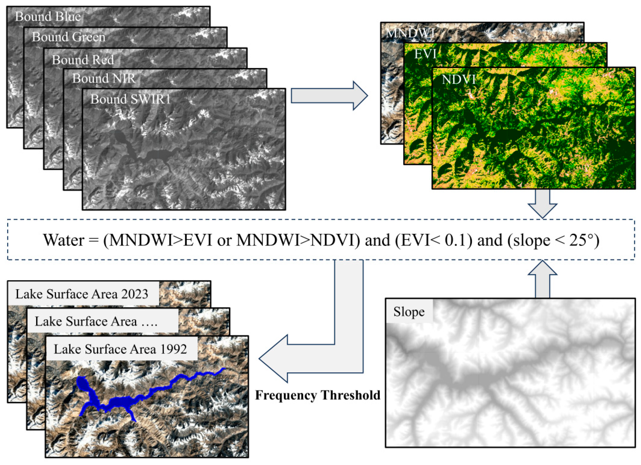
2.3.1. LSA Extraction

This study applied a multi-index threshold method (Figure 4) that integrated the modified normalized difference water index (MNDWI) [64], enhanced vegetation index (EVI) [65], and normalized difference vegetation index (NDVI) [66] to enhance water body extraction [67]. MNDWI has been extensively applied in the extraction of water bodies [64], and studies have shown that combining MNDWI with other indices, such as MNDWI > EVI or MNDWI > NDVI, more effectively distinguishes water bodies from non-water bodies [68]. Additionally, applying an EVI threshold of less than 0.1 effectively filters out vegetation pixels and those containing a mix of water and vegetation [69]. Ultimately, pixels that fulfill both the (MNDWI > EVI or MNDWI > NDVI) and (EVI < 0.1) conditions are classified as water bodies. This efficient and simple method can be quickly and reliably applied to all available images for subsequent water body frequency calculations. It has been extensively used for surface water and lake extraction in regions with diverse climatic conditions, such as the Inner Mongolia Plateau [69], Central Asia [70], and the headwater areas of the Three Rivers on the Qinghai–Tibet Plateau [71]. The formulae for these methods are as follows:

$$NDVI={\displaystyle \frac{\rho NIR-\rho Red}{\rho NIR+\rho Red}}$$

(1)

$$MNDWI={\displaystyle \frac{\rho Green-\rho SWIR1}{\rho Green+\rho SWIR1}}$$

(2)

$$EVI=2.5\times {\displaystyle \frac{\rho NIR-\rho Red}{1.0+\rho NIR+6.0\rho Red+7.5\rho Blue}}$$

(3)

where $\rho$_Blue, $\rho$_Green, $\rho$_Red, $\rho$_NIR, and $\rho$_SWIR1 represent the reflectance in the blue (0.45–0.52 μm), green (0.52–0.60 μm), red (0.63–0.69 μm), near-infrared (0.77–0.90 μm), and shortwave infrared 1 (1.55–1.75 μm) bands.

However, mountain shadows in optical imagery often exhibit spectral similarities to surface water, making water body detection more challenging, particularly in alpine regions [71,72]. DEM is widely recognized as an effective tool for eliminating mountain shadows and improving water extraction accuracy [73]. A slope mask generated from the ALOS World 3D-30m (AW3D30) DEM was applied in this study to filter out mountain shadows. AW3D30, part of the same series as the previously mentioned AW3D-5m DEM, has a 30 m resolution and can be accessed through the GEE platform [74]. Lake Sarez, a high-altitude landslide-dammed lake, is surrounded by steep mountains with an average slope of 23.67° [37]. Using a lower slope mask threshold (e.g., 5–10°) could effectively remove shadows but may also exclude water bodies near the mountain base [75]. To address this, the threshold was adjusted to 25° through trial and error, and visual quality control. After the slope mask was applied, pixels meeting the criteria in Equation (4) were identified as water bodies, while the remaining ones were classified as non-water bodies.

$$Water=\left(MNDWI>EVIorMNDWI>NDVI\right)and\left(EVI<0.1\right)and\left(Slope<25°\right)$$

(4)

Lake Sarez’s LSA tends to be larger in summer and autumn compared to winter and spring [36]; therefore, using a specific month or season to represent the annual lake surface area would not provide an accurate measure. Therefore, we employed the frequency method. For each pixel in the lake area, we assigned a value of 1 to the water pixels and 0 to the other pixels. Subsequently, the annual water frequency (F) for each pixel was computed using Equation (5).

$$F\left(y\right)={\displaystyle \frac{1}{N_y}}\sum _{i=1}^{N_y}{w}_{y,i}\times 100\%$$

(5)

where F represents the pixel’s water frequency, y represents the specified year, N_y represents the total Landsat observations for that pixel during the given year, and w_y,i indicates whether the pixel was classified as water (1 for water and 0 for non-water).

Based on previous studies and visual quality control, this study employed a 68% threshold for F to classify permanent and seasonal water bodies, which is particularly suitable for extracting lake areas in Central Asia [17]. Therefore, pixels with F ≥ 68% were identified as stable lake water bodies representing the LSA for that year. All the processes were conducted using the GEE platform.

2.3.2. Accuracy Validation of LSA Extraction

In this study, the algorithm was enhanced by incorporating a slope mask and adjusting thresholds to better accommodate the characteristics of high-altitude landslide-dammed lakes. The accuracy of the refined algorithm was verified by comparing its results with those obtained from high-resolution Google Earth images. First, a 90 m buffer zone was established around the extracted lake water area, defined as the Region of Interest (ROI). Next, using an equal-stratified random sampling method, 500 sample points were chosen at random within the ROI, comprising 250 water samples and 250 non-water samples, which were subsequently interpreted visually using ground-truth data from Google Earth. Finally, a confusion matrix was generated to calculate Overall Accuracy (OA), Producer’s Accuracy (PA), User’s Accuracy (UA), and the Kappa coefficient, in order to evaluate the accuracy of LSA extraction and validate the effectiveness of the improved algorithm.

Table 3. Accuracy validation results of confusion matrix for LSA extraction from Lake Sarez.

Sample Points	Google Earth Reference Data		Total
	Water	Non-Water
Water	245	5	250
Non-Water	10	240	250
Total	255	245	500

showed the confusion matrix results, indicating that the majority of sample points were accurately categorized as either water or non-water, demonstrating that the improved multi-index threshold method achieved high accuracy in extracting the LSA of Lake Sarez. The method attained an OA of 97.00% and a Kappa coefficient of 0.94, indicating a strong agreement with the reference data [76]. The method also achieved a PA of 96.08% for water and 97.96% for non-water, and a UA of 98.00% for water and 96.00% for non-water, confirming its high precision in delineating lake and non-lake areas. In comparison, the original multi-index threshold algorithm achieved a 96% overall accuracy and a Kappa coefficient of 0.94 [67]. This comparison highlighted the suitability of the improved method for accurately extracting the LSA of high-altitude lakes such as Lake Sarez, especially in challenging terrains and conditions. Compared with existing studies, such as the evaluation of 10 water extraction algorithms for Tibetan Plateau lakes using Landsat 9 imagery by Li et al. [77], where the best-performing Random Forest algorithm achieved 95.84% overall accuracy and a Kappa value of 0.91, Chen et al. [78], using Landsat 8 imagery and an improved NDWI for glacier lake extraction, achieved an overall accuracy of 97.70% and a Kappa value of 0.95, the accuracy in this study is comparable, demonstrating the reliability of the results.

The extracted LSA of Lake Sarez was further validated for temporal reliability by comparing it to the observed annual maximum lake level from 2005 to 2023. As shown in Figure 5, the extracted LSA exhibited strong consistency with the observed maximum lake levels, demonstrating a significant Pearson correlation coefficient of 0.802 (p < 0.01). This robustly confirmed the high accuracy and reliability of the extracted LSA, rendering it suitable for subsequent research.

2.3.3. Reconstruction of the Temporal Variation of Absolute LWS

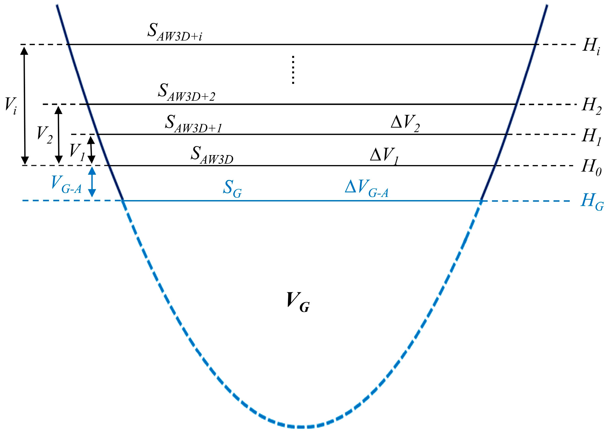
Using the GLOBathy bathymetry dataset, underwater depth data for Lake Sarez were obtained, and the lake basin volume was calculated using ArcGIS’s “Area and Volume” function to determine the absolute LWS (V_G). At this point, the corresponding LSA was 84.43 km², denoted as S_G. As the extracted LSA of Lake Sarez always exceeded the S_G, this study established a relationship model between the LSA and DEM-derived elevation to estimate water storage changes. There is a notable connection between the elevation of the lake and its surface area, and, assuming a regular basin shape, the above-water topography can be considered an extension of underwater topography [79]. As a high-altitude landslide-dammed lake, Lake Sarez’s basin is formed by surrounding mountains, with Google Earth images revealing a relatively regular “V” shape, indicating continuity between the above-water and underwater topography. Therefore, using high-resolution topographic data obtained from the AW3D-5m DEM, this study accurately modeled the relationship between LSA and elevation to estimate above-water storage changes and combined this with GLOBathy data to reconstruct the absolute LWS changes in Lake Sarez, as shown in Figure 6.

The steps for constructing the absolute LWS changes in Lake Sarez were as follows:

1.

The lake boundary was selected, and a 100 m buffer was created to define the DEM elevation search range.

2.

Extract contour lines using AW3D-5m DEM data, merge regions with the same elevation, and calculate the corresponding area for each elevation. The minimum elevation was set as H₀, and the corresponding area was set as S_AW3D.

3.

The elevation was increased from H₀ in 1 m increments up to 15 m, determining the relationship between each elevation Hi and the corresponding area S_AW3D+i (where i = 1, 2, …, 15), as shown in Table 4 (Columns 1 and 3).

4.

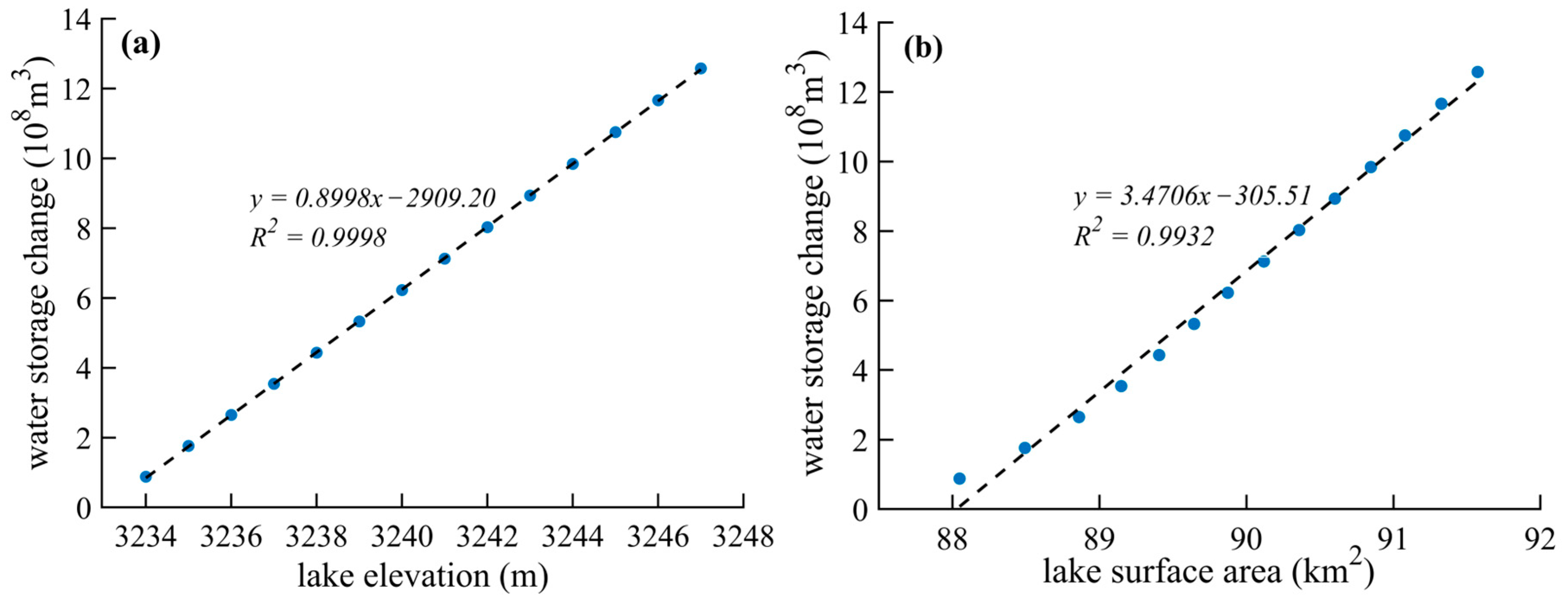
Using the elevation-area relationship, an empirical formula [80] (Equation (6)) was applied to calculate the variation in water storage for each H_i relative to H₀. This formula has been widely used in lake water storage assessments and is especially useful in remote areas lacking historical hydrological data [10,81,82]. A linear fitted formula (area–storage curve) was then established as ΔV = aS + b (Figure 7), as shown in Table 4 (Columns 3 and 5).

$$∆V={\displaystyle \frac{1}{3}}\left(H_i-H_0\right)\times \left(S_i+S_0+\sqrt{S_i\times S_0}\right)$$

(6)

where $∆$V is the LWS change, H_i and H₀ are the lake elevations, and S_i and S₀ are the LSA for the respective periods.

5.

The annually extracted LSA and S_G were substituted into the fitted formula from Step 4 to calculate the water storage change relative to S_AW3D as well as the volume change ∆V_G-A between S_G and S_AW3D. Finally, we added the annual water storage change ∆V_G-A and the underwater volume V_G to determine the absolute LWS for each year.

Figure 7. (a) Elevation–storage curve of Lake Sarez and (b) area–storage curve of Lake Sarez.

Figure 7. (a) Elevation–storage curve of Lake Sarez and (b) area–storage curve of Lake Sarez.

Table 4. Based on the correlation between elevation extracted from the AW3D-5m DEM and the LSA.

Elevation (m Above Sea Level)	Change in Lake Area per 1 m Elevation (km2)	Surface Area of Lake Sarez (km2)	Change in Water Storage at 1 m Interval (109 m3)	Change in Water Storage (109 m3)
3233	0	87.5631	0	0
3234	0.4853	88.0484	0.0878	0.0878
3235	0.4443	88.4927	0.0883	0.1761
3236	0.3681	88.8608	0.0887	0.2648
3237	0.2873	89.1481	0.0890	0.3538
3238	0.2580	89.4061	0.0893	0.4430
3239	0.2376	89.6437	0.0895	0.5326
3240	0.2294	89.8731	0.0898	0.6223
3241	0.2452	90.1183	0.0900	0.7123
3242	0.2401	90.3584	0.0902	0.8026
3243	0.2429	90.6013	0.0905	0.8930
3244	0.2451	90.8464	0.0907	0.9838
3245	0.2321	91.0785	0.0910	1.0747
3246	0.2475	91.3260	0.0912	1.1659
3247	0.2471	91.5731	0.0915	1.2574

Table 4. Based on the correlation between elevation extracted from the AW3D-5m DEM and the LSA.

Elevation (m Above Sea Level)	Change in Lake Area per 1 m Elevation (km2)	Surface Area of Lake Sarez (km2)	Change in Water Storage at 1 m Interval (109 m3)	Change in Water Storage (109 m3)
3233	0	87.5631	0	0
3234	0.4853	88.0484	0.0878	0.0878
3235	0.4443	88.4927	0.0883	0.1761
3236	0.3681	88.8608	0.0887	0.2648
3237	0.2873	89.1481	0.0890	0.3538
3238	0.2580	89.4061	0.0893	0.4430
3239	0.2376	89.6437	0.0895	0.5326
3240	0.2294	89.8731	0.0898	0.6223
3241	0.2452	90.1183	0.0900	0.7123
3242	0.2401	90.3584	0.0902	0.8026
3243	0.2429	90.6013	0.0905	0.8930
3244	0.2451	90.8464	0.0907	0.9838
3245	0.2321	91.0785	0.0910	1.0747
3246	0.2475	91.3260	0.0912	1.1659
3247	0.2471	91.5731	0.0915	1.2574

2.3.4. Water Balance Model of Lake Sarez

Lake water balance refers to the equilibrium between water inputs and outputs within a lake system, which determines changes in water storage and levels [83]. Constructing a lake water balance model allows for accurate assessment of storage changes and quantitative analysis of the driving factors [84]. Given the high-altitude location and minimal human activity in Lake Sarez, the impact of water extraction was negligible. Owing to the lack of groundwater data, this factor was incorporated into the uncertainty term, and the water balance equation for Lake Sarez over a given period can be expressed as follows [8]:

$${\displaystyle \frac{∆V}{∆t}}=S\left(P-E\right)+Q_{in}-Q_{out}+\epsilon$$

(7)

where $∆$t is the calculation period (years); $∆$V represents the LWS changes (m³); S represents the LSA (km²); E represents the total evaporation from the lake surface (mm); P represents the precipitation over the lake surface (mm); Q_in represents the inflow water volume (m³) and Q_out represents the outflow water volume (m³); and ε accounts for ungauged processes, including variations in groundwater and uncertainties in precipitation and evapotranspiration data (due to the absence of in situ measurements).

Using the observed inflow and outflow data from the Sarez Lake station in 2023, precipitation and evapotranspiration data from the TerraClimate dataset, and LSA extraction data from remote sensing, we constructed a water balance model for Lake Sarez for the same year. This model enabled us to conduct a quantitative evaluation of each factor’s contribution to LWS variation, identify dominant factors, and explore the underlying causes, offering deeper insights into the mechanisms of LWS variation.

2.3.5. Cross-Wavelet Transform and Wavelet Coherence

The cross-wavelet transform (XWT) combines wavelet transform and cross-spectral analysis, enabling the exploration of correlations between two time series within the time-frequency domain at various time scales. Higher XWT values indicate that the two time series share high-energy regions, suggesting a stronger correlation between them [85,86]. In this study, XWT was used to analyze the correlation between the dominant factors of absolute LWS and climate and atmospheric circulation factors across multiple timescales, highlighting their relationship in high-energy regions of the time–frequency domain. For two time series x(t) and y(t), the expression for XWT is as follows:

$$W_{XY}\left(a,\tau \right)=C_X\left(a,\tau \right)C_Y^{\mathrm{*}}\left(a,\tau \right)$$

(8)

where $W_{XY}(a,\tau )$ represents the XWT, and $C_X(a,\tau )$ represents the wavelet transform coefficient of x(t), while $C_Y^{*}(a,\tau )$ denotes the complex conjugate of y(t)’s wavelet transform coefficient, both at the scale parameter a and time shift parameter τ.

Wavelet coherence (WTC) measures the local interaction between two time series in the time–frequency domain, particularly emphasizing correlations within low-energy regions [87]. In this study, WTC was employed to analyze the local correlation between the dominant factors of absolute LWS and climate and atmospheric circulation factors in the time–frequency domain, particularly in areas where significant interactions may not be fully captured by high-energy regions. WTC is defined as follows:

$$R_n^2\left(s\right)={\displaystyle \frac{{\left|S\left[s^{-1}{W}_n^{xy}\left(s\right)\right]\right|}^2}{S\left(s^{-1}{\left|W_n^x\left(s\right)\right|}^2\right)·S\left(s^{-1}{\left|W_n^y\left(s\right)\right|}^2\right)}}$$

(9)

where S denotes the smoothing operator. The WTC value R² ranges from 0 to 1 and can be understood as a localized correlation coefficient within the time–frequency domain, with higher values indicating a stronger correlation.

In the plots of XWT and WTC, the black solid line shows the region influenced by edge effects, whereas the thick black contour outlines areas that have passed the 95% confidence threshold, as determined by the red noise test. The phase connection between the two time series is indicated by the arrows: → indicates in-phase variation, ← indicates anti-phase variation, ↑ indicates that the first series is ahead of the second by 90°, and ↓ indicates that the first series lags behind by 90° [88]. To evaluate how different factors influenced wavelet coherence, we also calculated the share of WTC values surpassing the 95% significance threshold across the full wavelet-scale domain. This proportion is defined as the percentage area of significant coherence (PASC), where a higher PASC signifies stronger coherence between the two factors, indicating a more substantial influence [89].

3. Results

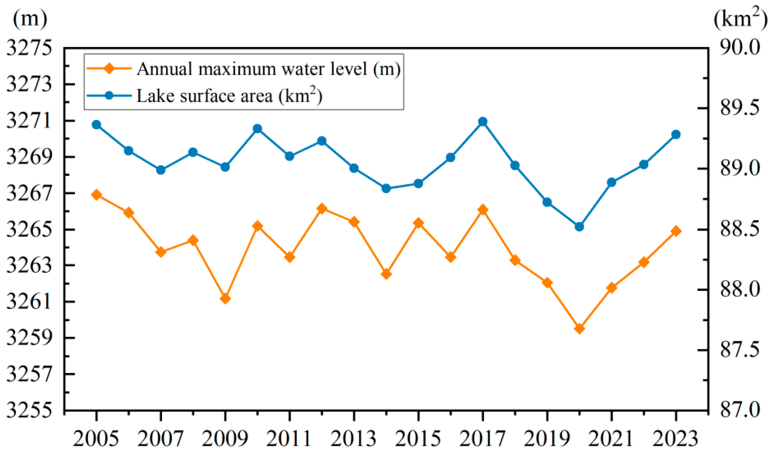
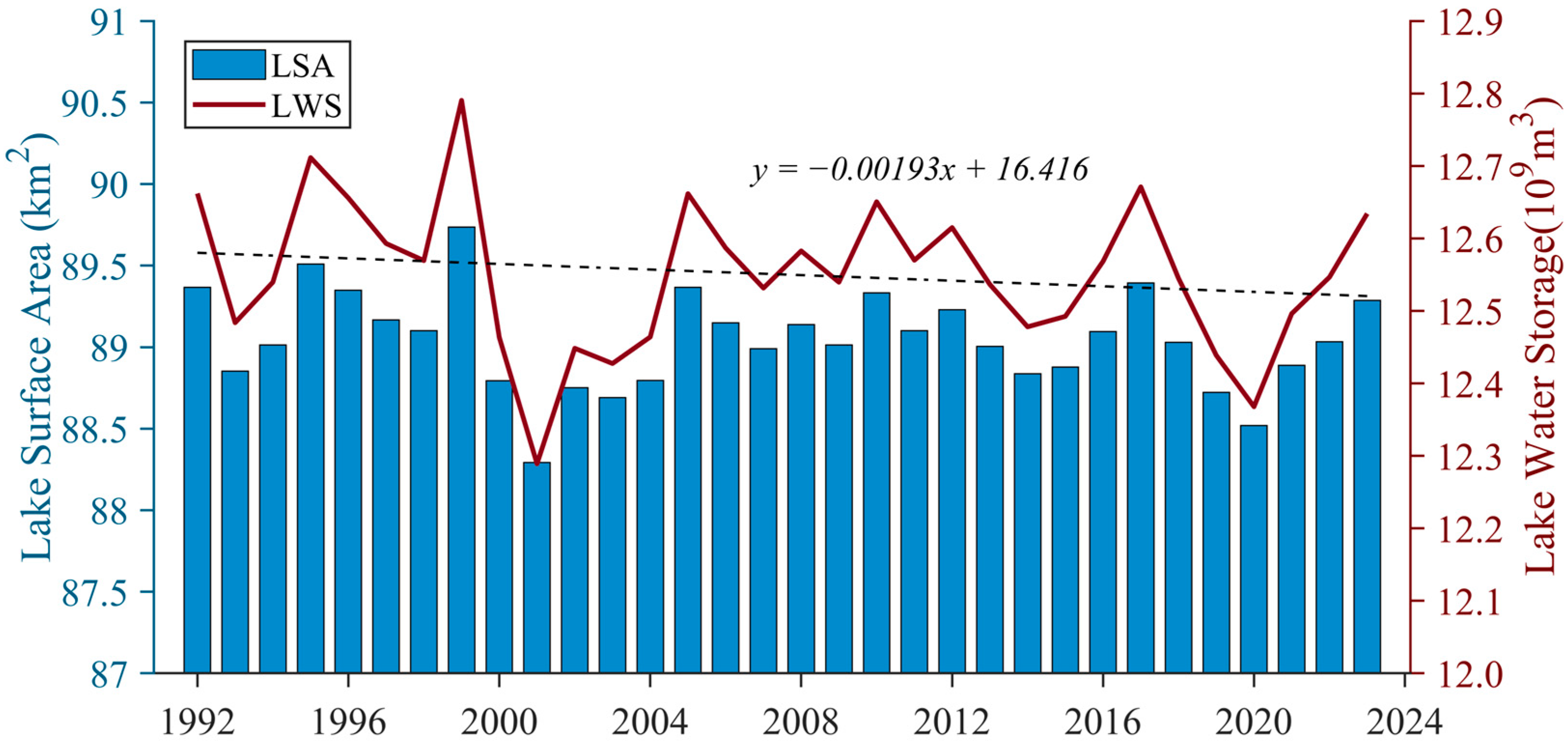
3.1. LSA and Absolute LWS Changes of Lake Sarez

Using bathymetric data and the area–storage curve (Table 4), we computed the absolute LWS changes in Lake Sarez from 1992 to 2023 (Figure 8). A strong linear relationship exists between the LWS and LSA, described by the equation y = 3.4715x − 183.61, with R² = 0.99. Over the past 32 years, the LSA of Lake Sarez has shown an overall slight decline, decreasing by 0.176 km² at a rate of 0.055 km² per decade. The average annual LSA is 89.04 km², with the largest LSA recorded in 1999 at 89.74 km² and the smallest in 2001 at 88.29 km², resulting in a range of only 1.45 km². Although the LSA of Lake Sarez remained relatively stable within a range of only 1.45 km², this does not imply that its hydrological characteristics were stable. As a deep lake, LSA changes do not fully capture hydrological dynamics, necessitating the further analysis of the absolute LWS changes. As shown by the folded line graph in Figure 8, the reconstructed absolute LWS ranged from approximately 12.3 × 10⁹ to 12.8 × 10⁹ m³. The absolute LWS and LSA change synchronously but with different magnitudes. The linear trend of the absolute LWS from 1992 to 2023 was negative. A Mann–Kendall trend test on the absolute LWS changes yielded a Z value of −0.92, below the 90% significance level, indicating a non-significant overall decrease over the past 32 years at a rate of −0.019 × 10⁹ m³ per decade. The annual average absolute LWS is 12.55 × 10⁹ m³, with the highest in 1999 at 12.79 × 10⁹ m³, and the lowest in 2001 at 12.29 × 10⁹ m³.

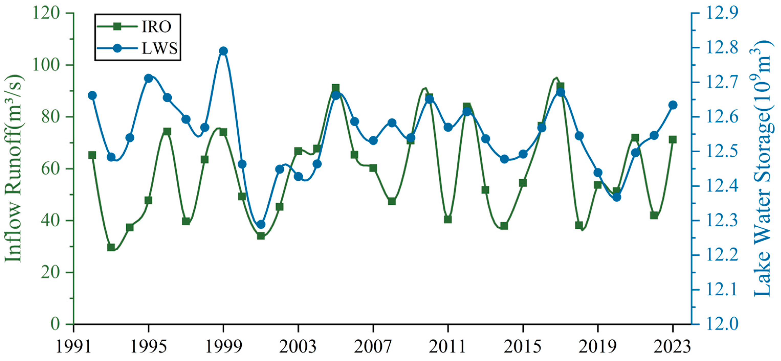
3.2. Dominant Factors of LWS Changes

LWS changes are a direct result of the water balance, and the interaction of water balance components determines these changes. In this study, the inflow, outflow, precipitation, and evapotranspiration were selected as the primary driving factors. Using 2023 as an example, the contribution rates of these factors to the absolute LWS changes in Lake Sarez were calculated using a contribution analysis (

Table 5. Statistical analysis of water balance factors and their contribution to LWS changes in Lake Sarez in 2023.

Factor	Value	Contribution	Contribution Rate
Annual Average Precipitation	216.00 mm	0.0193 km3	0.50%
Annual Average Evapotranspiration	207.34 mm	0.0185 km3	0.48%
Annual Average Inflow	66.54 m3/s	2.0984 km3	54.57%
Annual Average Outflow	54.20 m3/s	1.7093 km3	44.45%
Lake Surface Area	89.29 km2
Water Balance Change	0.3899 km3

). The results indicate the following: (1) Inflow was the dominant factor affecting the absolute LWS changes, with a contribution rate of 54.57%. (2) Runoff (inflow and outflow) had a significantly greater impact on absolute LWS changes than did meteorological factors (precipitation and evapotranspiration). Runoff contributed to 99% of the changes in LWS, whereas meteorological factors contributed only 1%. The limited contribution of meteorological factors to the overall changes in Lake Sarez’s LWS can be attributed to several key factors. First, because of the lake’s considerable depth and moderate surface area, the impact of surface-level precipitation and evaporation, both of which exhibit modest magnitudes, cannot significantly affect overall water storage. In contrast, inflow originates from a large catchment area, providing substantial runoff from snowmelt and precipitation. Therefore, runoff has a far more pronounced effect on the LWS of the lake than direct contributions from precipitation and evaporation.

Figure 9 shows the relationship between the inflow and absolute LWS over time, with both exhibiting relatively consistent temporal variations. A correlation analysis between the inflow and absolute LWS of Lake Sarez from 1992 to 2023 revealed a significant Pearson correlation (p < 0.01) and a coefficient of 0.51. Combined with its contribution rate of 54.57%, it is evident that the inflow has a decisive influence on the absolute LWS to some extent. The water balance results highlight the crucial role of runoff in changes in the lake water volume. Runoff directly influences both the water levels and storage capacity, with a typically positive correlation, particularly in lakes where runoff is the dominant contributor. In such cases, inflow variations largely determine the water volume. For example, the water level of Lake Baikal is primarily controlled by the inflow from its main tributary, the Selenga River [90]. Likewise, in Lake Balkhash, approximately 75% of the water originates from the Ili River. Following the 1970 construction of a reservoir on the Ili River, which diverted its flow, the water level of Lake Balkhash declined significantly and remained low for nearly a decade [91].

Although the outflow resulting from seepage also significantly affects the lake’s water storage, it has remained relatively stable over the past few decades [34]. The variation in seepage is primarily influenced by the water level of the lake: higher water levels result in greater seepage, whereas lower levels result in less seepage [32]. Given the clear understanding of these factors, further analysis of seepage was not conducted in this study.

In contrast, the inflow is affected more by meteorological factors within the watershed and shows more significant interannual fluctuations than the outflow. The mechanisms underlying these variations in the inflow are not well-understood. Therefore, to better understand the causes of absolute LWS changes, it is necessary to further analyze the factors influencing inflow, which is the dominant driver of these changes.

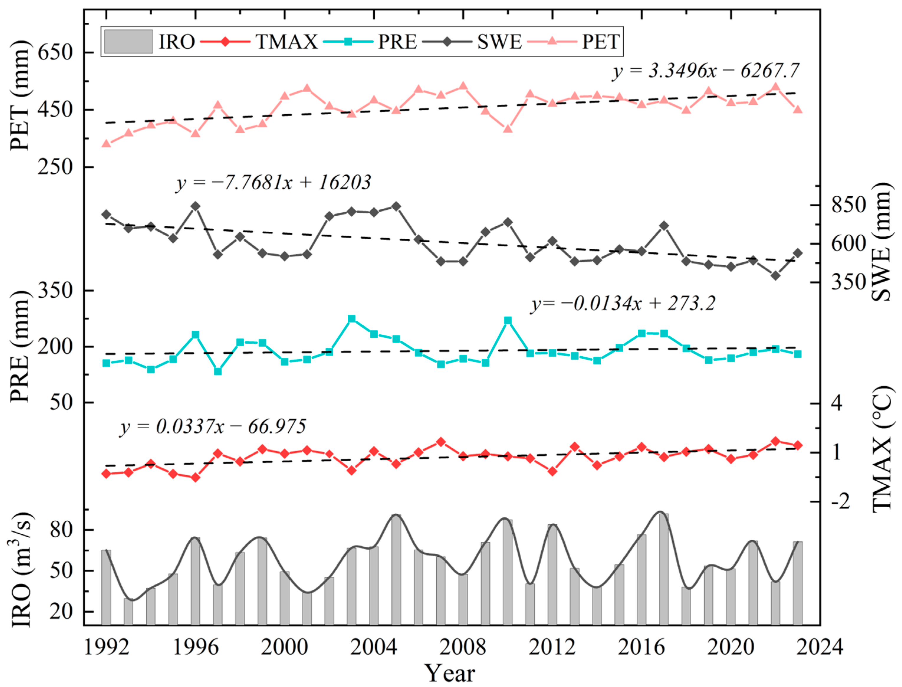
3.3. Climatic and Atmospheric Drivers of IRO Variations in Lake Sarez

3.3.1. Multi-Scale Correlation Analysis of Basin Climatic Factors and IRO in Lake Sarez

Lake inflow is significantly influenced by various climatic factors within the watershed. Temperature, precipitation, and evaporation are key drivers of runoff variability [92], whereas SWE impacts the inflow through its freeze–thaw effects. Figure 10 shows the interannual variations in IRO and climate factors for Lake Sarez from 1992 to 2023. Since 1992, the annual mean temperature in the watershed has increased by 0.34 °C per decade, exceeding the global average rise of 0.20 °C per decade [93]. During this period, PET increased by 3.35 mm per year, PRE fluctuated between 125 and 300 mm with a slight decline, and SWE showed a more pronounced decrease at −7.77 mm per year.

A Pearson correlation analysis identified significant relationships between IRO and PRE (r = 0.63, p < 0.01) and SWE (r = 0.44, p < 0.05) but no significant correlation with mean TMAX or PET. This preliminary analysis highlights the need for a further investigation of the climatic drivers of IRO. To this end, XWT and WTC were utilized to explore the time–frequency relationships of IRO with TMAX, PRE, PET, and SWE. XWT emphasizes the correlation between two signals in high-energy regions, uncovering the periods in which they exhibit significant shared power. In contrast, the WTC reflects the coherence in low-energy regions, indicating consistent phase relationships even in areas of lower power. The results are shown in Figure 11.

Figure 11a shows that TMAX and IRO exhibited a significant two-to-three-year resonance period in the high-energy region during 2011–2013, with TMAX leading IRO by approximately 90°. However, the area that passed the confidence test was small, indicating a weak influence. This is further supported by the WTC in Figure 11e, where only a small significant area around the two-to-three-year period was observed. This suggests that, while TMAX affects IRO, its impact is relatively weak. In contrast, Figure 11b reveals three significant resonance periods between PRE and IRO, with a prominent six-to-eight-year cycle during 2000–2016 showing a positive correlation. Figure 11f indicates that the significant region occupies a large portion of the cone of influence, with the main cycle of around five to nine years spanning almost the entire series from 1992 to 2023. Coherence coefficients were generally above 0.8, with some reaching close to 1, indicating a strong and sustained positive relationship. This underscores PRE as a major influencing factor on IRO with a lasting impact. Similar to the PRE, Figure 11c,g demonstrate that SWE is closely linked to IRO. They share two significant resonance periods in the high-energy region with positive phase relationships, particularly in the main six-to-eight-year cycle from 1999 to 2015, where the interaction is strongest. In the low-energy region, three resonance periods with varying but generally positive correlations were observed within the cone of influence, suggesting that SWE is also a significant positive factor affecting the IRO. Figure 11d,h show the anti-phase relationship between PET and IRO, which indicates a negative impact. The downward-sloping arrows suggest that the IRO lagged behind the PET changes, which is aligned with the expected physical relationship.

The analysis indicated that the IRO of Lake Sarez was influenced to varying degrees by four climatic factors. The PASC values for the WTC analysis between IRO and TMAX, PRE, SWE, and PET were 2.18%, 48.33%, 27.92%, and 20.93%, respectively. Overall, PRE and SWE were the primary factors affecting IRO, and both showed a positive correlation with IRO, with PRE having a more sustained impact. PET negatively impacts IRO and interacts with other factors that influence IRO. For example, during 1999–2001, an increase in PET along with decreases in PRE and SWE likely contributed to the reduction in IRO, causing a decline in the LWS, and the effect of temperature on IRO is more complex. On one hand, rising temperatures can accelerate snow and ice melt, providing more water to rivers; on the other hand, higher temperatures also increase evaporation. Although no direct link was found between temperature and IRO changes, there was a strong correlation between temperature and both PET and SWE, with Pearson correlation coefficients of −0.61 (p < 0.01) and −0.59 (p < 0.01), respectively. This suggests that temperature indirectly influences IRO by affecting the PET and SWE.

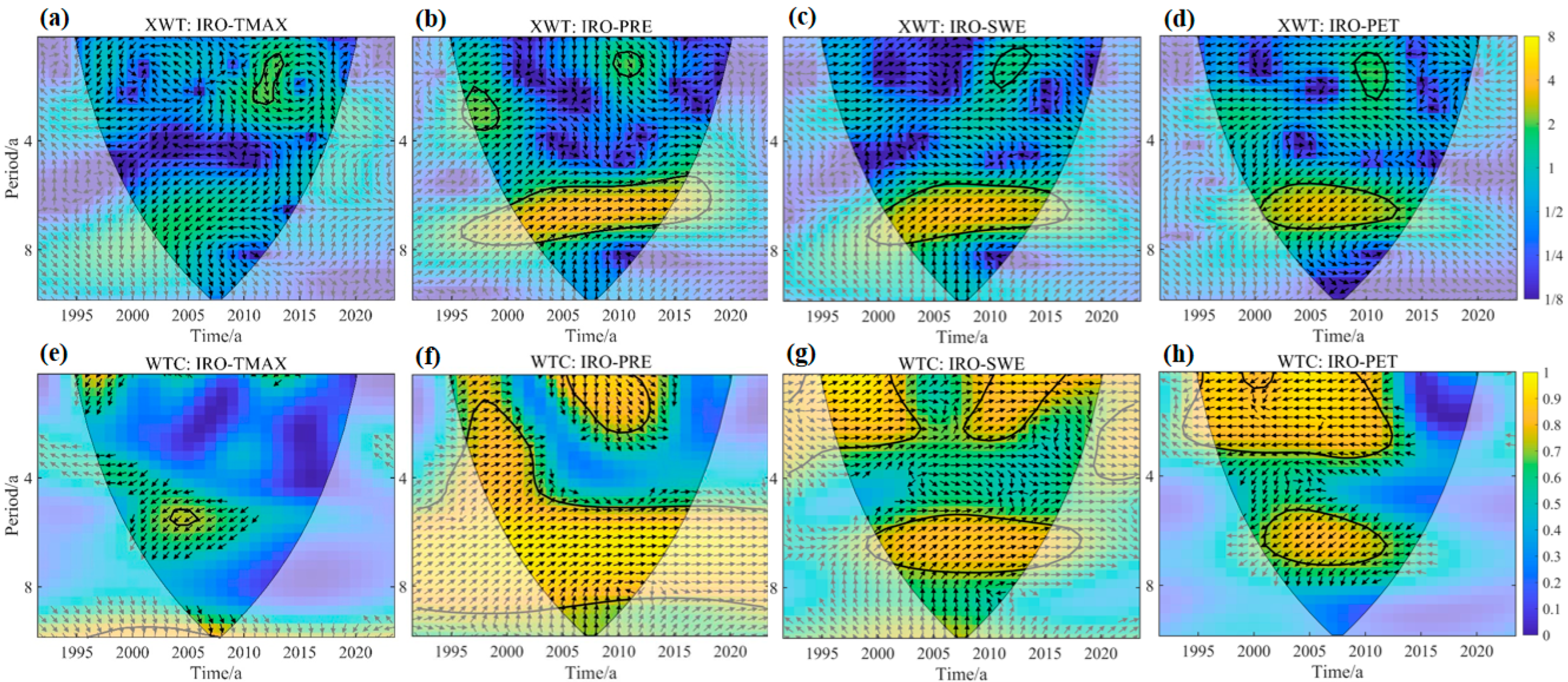
3.3.2. Multi-Scale Teleconnection Analysis of Atmospheric Circulation and IRO in Lake Sarez

Large-scale atmospheric circulation can have a profound impact on regional climate, particularly on temperature and precipitation, thereby affecting the seasonal and yearly distribution of runoff [94]. Studies have shown that circulation factors such as NAO, NINO3.4, TPI, and PDO have significant impacts on the hydroclimate of Central Asia [95]. In this study, CWT and WTC were utilized to investigate the connections between IRO and these four large-scale circulation indices.

XWT and WTC revealed complex relationships between IRO and atmospheric circulation factors across different time scales in both high- and low-energy regions (Figure 12). In high-energy regions, TPI and IRO exhibited two significant resonance periods; however, the area of significance was very small. In the low-energy regions, they showed a positive correlation at the one-to-two-year and five-to-six-year resonance periods, particularly during the one-to-two-year period when the correlation coefficient exceeded 0.9. This indicates that TPI exerted a significantly positive influence on IRO between 2011 and 2013. NINO3.4 and IRO displayed three notable resonance periods within the high-energy regions, with the strongest resonance occurring over the six-to-seven-year period (2001–2008). In the low-energy regions, significant coherence is observed at the six-to-eight-year time scale during 2001–2009, with phase arrows pointing upward to the right at approximately 45°, indicating that IRO leads NINO3.4 by approximately one year. PDO and IRO exhibited three notable resonance periods within the high-energy regions, but the energy intensity was relatively low. Three distinct resonance periods were observed in the low-energy regions, with the zero-to-three-year period (2005–2015) having the largest area and the highest coherence coefficient. However, no clear positive or negative correlation is observed, with arrows pointing downward, indicating that the IRO lags behind the PDO by approximately one year. NAO and IRO did not exhibit significant resonance periods in the high-energy regions; however, in the low-energy regions, a significant resonance period was observed at the two-to-four-year scale during 2010–2016, showing a significant negative correlation, suggesting that IRO was notably influenced by NAO during this period. Additionally, a Pearson correlation analysis between IRO and NAO from 1992 to 2023 yielded a coefficient of −0.45 (p < 0.01), indicating a strong overall negative correlation throughout the study period.

The above analysis indicates that IRO and various circulation factors have different resonance periods and time lags in the time–frequency domain, with varying degrees of correlation. TPI, NINO3.4, PDO, and NAO mainly influenced IRO at different scales during 2011–2013, 2001–2008, 2005–2015, and 2010–2016, respectively. Additionally, the PDO displayed higher PASC values than other atmospheric circulation indices, suggesting a stronger influence on IRO variations. In contrast, NAO showed a significant negative correlation with IRO in low-energy regions, despite not showing significant resonance periods in high-energy regions, suggesting that it also plays an important role in influencing the runoff variability.

4. Discussion

4.1. Innovation and Uncertainty in the Reconstruction of Absolute LWS for Landslide-Dammed Lakes

In this study, we successfully reconstructed the annual LSA and absolute LWS changes in Lake Sarez from 1992 to 2023, a poorly documented high-altitude landslide-dammed lake, using multi-source remote sensing data (including all available Landsat images and the GLOBathy global lake bathymetry dataset combined with the high-resolution AW3D-5m DEM). To improve the accuracy of LSA extraction for Lake Sarez, we adapted the water extraction algorithm for cold regions proposed by Zou et al. [67] by incorporating a 25° slope mask and 68% threshold, considering the specific environmental characteristics of Lake Sarez. This approach provided reliable data for the reconstruction of water storage in high-altitude landslide-dammed lakes. The extracted LSA data were combined with underwater bathymetry and above-water DEM data to construct the absolute LWS change curve. This innovative method offers a high estimation accuracy, filling the gap in the annual LSA and absolute LWS changes for Lake Sarez, and provides a new approach for hydrological studies of other high-altitude landslide-dammed lakes. We cautiously suggest that this improved method for reconstructing LWS is applicable to landslide-dammed lakes in high-altitude regions, and could be extended to the Tibetan Plateau and other similar lakes worldwide.

However, there were two main sources of uncertainty in this study. The first was the limited availability of Landsat images in the initial years of the study period, such as between 1992 and 2003, when fewer images were available compared with later periods. This lack of image data may result in a lower accuracy in early LSA extraction, thereby affecting the accuracy of the reconstructed water storage. Cloud contamination in Landsat imagery also affects LSA extraction. Although we employed the CFmask algorithm for cloud removal and used all available Landsat images to minimize the impact of images with heavy cloud coverage, it remains challenging to fully replicate the actual conditions. In addition, uncertainty in the GLOBathy bathymetry data could have affected the accuracy of the reconstructed water storage data. Although the GLOBathy bathymetry data were generated using a random forest regression model and have been validated, errors may still occur, particularly in areas with complex terrain and deep lakes, where the bathymetry data may not fully capture the fine-scale variations in the lakebed topography, thereby affecting the accuracy of the water storage estimation. Therefore, future research should focus on overcoming the challenges posed by the low image quality. Moreover, the introduction of advanced remote sensing technologies and geophysical measurement methods, such as LiDAR and high-resolution sonar, could enhance the accuracy of the bathymetric and surface topography data of lakes, leading to more precise calculations of the actual lake volume and reducing the discrepancy in LWS change estimates. Owing to a lack of groundwater data, its impact was not incorporated into the lake water balance model. Future studies could refine the model by incorporating in situ groundwater monitoring or coupled hydrological models to better quantify this factor and reduce uncertainty.

4.2. Insights into Lake Sarez’s Absolute LWS Changes

Changes in the LWS are essential responses to climate change [15]. For Lake Sarez, variations in the inflow runoff were the primary drivers of absolute LWS changes. This study utilized XWT and WTC to investigate how meteorological and atmospheric circulation factors influence the runoff, revealing how climate change influences LWS. During the study period, the absolute water storage in Lake Sarez declined slightly. The precipitation and snow–water equivalent were the main meteorological factors that directly and indirectly affected the inflow runoff. The decline in water storage was primarily attributed to a decrease in these factors. While the direct impact of temperature was weaker, it remained significant through its effects on precipitation and the snow–water equivalent. A warming of 1.2 °C over the past 70 years has led to a 20% reduction in snow depth in the mountainous regions of Central Asia [96]. Snowmelt is a crucial source of runoff in the Pamir Plateau, and the reduction in snow depth directly influences runoff, which, in turn, impacts the LSA and LWS of Lake Sarez. Additionally, a decline in the ratio of snowfall to total precipitation in the eastern Pamirs [97], where Lake Sarez is located, has resulted in reduced snow and glacier accumulation during the winter months, which has further affected the LWS variations. While rising temperatures may initially increase the glacial meltwater runoff, as glaciers retreat, their contribution to the runoff diminishes [98]. This is consistent with the findings of Liu et al. [2], who observed that, in some alpine lakes in Central Asia, precipitation plays a more significant role than glacier meltwater in lake recharge.

Atmospheric circulation factors, including TPI, NINO3.4, PDO, and NAO, significantly impacted the Lake Sarez inflow runoff. A WTC analysis revealed significant resonance periods between these factors and the inflow runoff, indicating that changes in regional and global climate systems influence LWS by affecting the precipitation and runoff. This study emphasizes the intricate impacts of climate change on the hydrological processes of high-altitude lakes. The decline in the precipitation and snow–water equivalent directly reduced LWS, while the indirect effects of temperature and atmospheric circulation were also important. Future research should continue to monitor these climatic factors and their combined impacts on LWS to provide crucial insights for regional water resource management and ecological conservation.

Since the formation of Lake Sarez, the LWS has generally exhibited a fluctuating upward trend [30]. This study revealed that, over the past three decades, the rate of increase in LWS has decelerated, with a slight decrease noted in recent years. This observation does not justify any relaxation in the monitoring and management efforts. Currently, the lake is still at a historically high LWS, which exerts significant pressure on the natural dam at Usoi, and the risk of breach remains. Although precipitation during the study period has remained relatively stable with a slight downward trend, studies suggest that precipitation in the eastern Pamirs, including in the Lake Sarez watershed, is expected to increase in the future [99]. This increase in precipitation will likely enhance the inflow runoff into the lake, and the accumulation of precipitation will also help offset the glacier retreat caused by rising temperatures. Therefore, in the future, the LWS of Lake Sarez may continue to increase, further exacerbating the stability risks to the dam.

Given the potential fluctuations in the LWS due to climate change, it is essential to develop effective response strategies. These strategies can help strengthen water resource management and regional safety. One approach could involve constructing a hydropower station at Lake Sarez, where the LWS could be controlled and lowered to mitigate the risk of a lake breach [34]. Additionally, a water flow control system can be implemented to manage resources effectively, thereby increasing reservoir storage during high-flow periods to ensure water availability for downstream needs during dry spells. Furthermore, to address the uncertainties caused by climate change, it is necessary to strengthen the real-time monitoring and early warning systems for climate and hydrological changes. Given that runoff is a primary driver of LWS changes, local water managers should further enhance the accuracy and consistency of the field monitoring of the inflow and outflow runoff. This will effectively capture the overall water balance of the lake, enabling timely intervention and informed decision-making. By integrating the cycles driven by circulation factors and based on the mechanisms of the NINO, TPI, NAO, and PDO, it is possible to predict periods of increased runoff in advance and implement appropriate warning and response measures.

5. Conclusions

In this study, all available Landsat imagery, the GLOBathy bathymetry dataset, and the high-resolution AW3D 5m DEM were used to reconstruct the absolute LWS of Lake Sarez from 1992 to 2023 and to analyze its changing characteristics and driving factors under the influence of climate change. The conclusions are as follows:

The LSA extracted using the improved multi-index threshold method achieved a high accuracy, with a Kappa coefficient of 0.94 and a strong Pearson correlation coefficient of 0.802 with observed lake levels. During the study period, the average annual LSA of Lake Sarez was 89.04 km², indicating a slight declining trend, and the absolute LWS fluctuated between 12.3 × 10⁹ and 12.8 × 10⁹ m³, with an average of 12.55 × 10⁹ m³.

These findings highlight the sensitivity of Lake Sarez to global climatic variability. The water balance results indicate that IRO is the primary driver of absolute LWS changes in Lake Sarez. XWT and WTC analyses showed that PRE and SWE were the key climatic factors influencing the interannual variation in IRO, and both were positively correlated with IRO, with PRE having a more sustained impact. PRE and SWE significantly affect the IRO through direct contributions and snowmelt processes, thereby influencing the lake’s absolute LWS. Temperature indirectly regulates IRO by affecting SWE and PET. Moreover, IRO and various atmospheric circulation factors have different resonance periods and time lags in the time–frequency domain. The interannual variations in the IRO were primarily influenced by the PDO and NAO circulation patterns. PDO shows a longer resonance period with IRO, with IRO lagging behind PDO by approximately one year. In contrast, NAO displayed a significant negative correlation with IRO, indirectly affecting the runoff through regional climate modulation.

The findings of this study provide crucial fundamental data to support water management and risk assessments for Lake Sarez, along with novel insights into the effects of climate change on high-altitude lake hydrology, thereby providing a foundation for formulating ecological protection strategies. This methodology can be extended to dynamically monitor lakes on the Pamir Plateau, thereby enhancing the understanding of how lakes on the Pamir Plateau respond, particularly barrier lakes, to global changes.

References

1. Zhou, J.; Wang, L.; Zhong, X.; Yao, T.; Qi, J.; Wang, Y.; Xue, Y. Quantifying the Major Drivers for the Expanding Lakes in the Interior Tibetan Plateau. Sci. Bull. 2022, 67, 474–478. [Google Scholar] [CrossRef]
2. Liu, H.; Chen, Y.; Ye, Z.; Li, Y.; Zhang, Q. Recent Lake Area Changes in Central Asia. Sci. Rep. 2019, 9, 16277. [Google Scholar] [CrossRef] [PubMed]
3. El-Bouhali, B.; Mhamed, A.; Ech-Chahdi, K.E.O. Changes in Water Surface Area of the Middle Atlas-Morocco Lakes: A Response to Climate and Human Effects. Int. J. Eng. Geosci. 2024, 9, 221–232. [Google Scholar] [CrossRef]
4. Zhang, G.; Yao, T.; Xie, H.; Yang, K.; Zhu, L.; Shum, C.K.; Bolch, T.; Yi, S.; Allen, S.; Jiang, L.; et al. Response of Tibetan Plateau Lakes to Climate Change: Trends, Patterns, and Mechanisms. Earth-Sci. Rev. 2020, 208, 103269. [Google Scholar] [CrossRef]
5. Woolway, R.I.; Kraemer, B.M.; Lenters, J.D.; Merchant, C.J.; O’Reilly, C.M.; Sharma, S. Global Lake Responses to Climate Change. Nat. Rev. Earth Environ. 2020, 1, 388–403. [Google Scholar] [CrossRef]
6. Wang, W.; Jiao, A.; Shan, Q.; Wang, Z.; Kong, Z.; Ling, H.; Deng, X. Expansion of Typical Lakes in Xinjiang under the Combined Effects of Climate Change and Human Activities. Front. Environ. Sci. 2022, 10, 1015543. [Google Scholar] [CrossRef]
7. Tan, C.; Guo, B.; Kuang, H.; Yang, H.; Ma, M. Lake Area Changes and Their Influence on Factors in Arid and Semi-Arid Regions along the Silk Road. Remote Sens. 2018, 10, 595. [Google Scholar] [CrossRef]
8. Wang, X.; Huang, Y.; Liu, T.; Li, J.; Wang, Z.; Zan, C.; Duan, Y. Analysis of Water Balance Change and Influencing Factors in Issyk-Kul Lake in Recent 60 Years. AZR 2022, 39, 1576–1587. [Google Scholar] [CrossRef]
9. Adrian, R.; O’Reilly, C.M.; Zagarese, H.; Baines, S.B.; Hessen, D.O.; Keller, W.; Livingstone, D.M.; Sommaruga, R.; Straile, D.; Van Donk, E.; et al. Lakes as Sentinels of Climate Change. Limnol. Oceanogr. 2009, 54, 2283–2297. [Google Scholar] [CrossRef] [PubMed]
10. Zhang, G.; Bolch, T.; Chen, W.; Crétaux, J.-F. Comprehensive Estimation of Lake Volume Changes on the Tibetan Plateau during 1976–2019 and Basin-Wide Glacier Contribution. Sci. Total Environ. 2021, 772, 145463. [Google Scholar] [CrossRef] [PubMed]
11. Zhang, Y.; An, C.; Zheng, L.; Liu, L.; Zhang, W.; Lu, C.; Zhang, Y. Assessment of Lake Area in Response to Climate Change at Varying Elevations: A Case Study of Mt. Tianshan, Central Asia. Sci. Total Environ. 2023, 869, 161665. [Google Scholar] [CrossRef]
12. Zhang, R.; Zhu, L.; Ma, Q.; Chen, H.; Liu, C.; Zubaida, M. The Consecutive Lake Group Water Storage Variations and Their Dynamic Response to Climate Change in the Central Tibetan Plateau. J. Hydrol. 2021, 601, 126615. [Google Scholar] [CrossRef]
13. Jungkeit-Milla, K.; Pérez-Cabello, F.; De Vera-García, A.V.; Galofré, M.; Valero-Garcés, B. Lake Surface Water Temperature in High Altitude Lakes in the Pyrenees: Combining Satellite with Monitoring Data to Assess Recent Trends. Sci. Total Environ. 2024, 933, 173181. [Google Scholar] [CrossRef]
14. Drenkhan, F.; Guardamino, L.; Huggel, C.; Frey, H. Current and Future Glacier and Lake Assessment in the Deglaciating Vilcanota-Urubamba Basin, Peruvian Andes. Glob. Planet. Change 2018, 169, 105–118. [Google Scholar] [CrossRef]
15. Qiao, B.; Zhu, L.; Wang, J.; Ju, J.; Ma, Q.; Liu, C. Estimation of Lakes Water Storage and Their Changes on the Northwestern Tibetan Plateau Based on Bathymetric and Landsat Data and Driving Force Analyses. Quat. Int. 2017, 454, 56–67. [Google Scholar] [CrossRef]
16. Wang, W.; Zhang, F.; Shi, J.; Zhao, Q.; Liu, C.; Tan, M.L.; Kung, H.-T.; Gao, G.; Li, G. Calculation of Bosten Lake Water Storage Based on Multiple Source Remote Sensing Imagery. IEEE Trans. Geosci. Remote Sens. 2024, 62, 5100511. [Google Scholar] [CrossRef]
17. Huang, W.; Duan, W.; Chen, Y. Unravelling Lake Water Storage Change in Central Asia: Rapid Decrease in Tail-End Lakes and Increasing Risks to Water Supply. J. Hydrol. 2022, 614, 128546. [Google Scholar] [CrossRef]
18. Bai, J.; Chen, X.; Yang, L.; Fang, H. Monitoring Variations of Inland Lakes in the Arid Region of Central Asia. Front. Earth Sci. 2012, 6, 147–156. [Google Scholar] [CrossRef]
19. Navruzshoev, H.; Sagintayev, Z.; Kabutov, H.; Nekkadamova, N.M.; Vosidov, F.; Khalimov, A. Surface Area Dynamics of Gunt River Basin Mountain Lakes (Pamir, Tajikistan). Cent. Asian J. Water Res. 2022, 8, 141–152. [Google Scholar] [CrossRef]
20. Zheng, G.; Bao, A.; Li, J.; Zhang, G.; Xie, H.; Guo, H.; Jiang, L.; Chen, T.; Chang, C.; Chen, W. Sustained Growth of High Mountain Lakes in the Headwaters of the Syr Darya River, Central Asia. Glob. Planet. Change 2019, 176, 84–99. [Google Scholar] [CrossRef]
21. Du, W.; Pan, Y.; Li, J.; Bao, A.; Chai, H.; Yuan, Y.; Cheng, C. Glacier Retreat Leads to the Expansion of Alpine Lake Karakul Observed Via Remote Sensing Water Volume Time Series Reconstruction. Atmosphere 2023, 14, 1772. [Google Scholar] [CrossRef]
22. Zhang, Y.; Wang, N.; Yang, X.; Mao, Z. The Dynamic Changes of Lake Issyk-Kul from 1958 to 2020 Based on Multi-Source Satellite Data. Remote Sens. 2022, 14, 1575. [Google Scholar] [CrossRef]
23. Zhu, S.; Liu, B.; Wan, W.; Xie, H.; Fang, Y.; Chen, X.; Li, H.; Fang, W.; Zhang, G.; Tao, M.; et al. A New Digital Lake Bathymetry Model Using the Step-Wise Water Recession Method to Generate 3D Lake Bathymetric Maps Based on DEMs. Water 2019, 11, 1151. [Google Scholar] [CrossRef]
24. Jawak, S.D.; Vadlamani, S.S.; Luis, A.J. A Synoptic Review on Deriving Bathymetry Information Using Remote Sensing Technologies: Models, Methods and Comparisons. Adv. Remote. Sens. 2015, 04, 147–162. [Google Scholar] [CrossRef]
25. Khazaei, B.; Read, L.K.; Casali, M.; Sampson, K.M.; Yates, D.N. GLOBathy, the Global Lakes Bathymetry Dataset. Sci. Data 2022, 9, 36. [Google Scholar] [CrossRef]
26. Yuan, C.; Zhang, F.; Liu, C. A Comparison of Multiple DEMs and Satellite Altimetric Data in Lake Volume Monitoring. Remote Sens. 2024, 16, 974. [Google Scholar] [CrossRef]
27. Lei, Y.; Tian, L.; Bird, B.W.; Hou, J.; Ding, L.; Oimahmadov, I.; Gadoev, M. A 2540-Year Record of Moisture Variations Derived from Lacustrine Sediment (Sasikul Lake) on the Pamir Plateau. Holocene 2014, 24, 761–770. [Google Scholar] [CrossRef]
28. Mętrak, M.; Szwarczewski, P.; Bińka, K.; Rojan, E.; Karasiński, J.; Górecki, G.; Suska-Malawska, M. Late Holocene Development of Lake Rangkul (Eastern Pamir, Tajikistan) and Its Response to Regional Climatic Changes. Palaeogeogr. Palaeoclimatol. Palaeoecol. 2019, 521, 99–113. [Google Scholar] [CrossRef]
29. Costa, J.E.; Schuster, R.L. Documented Historical Landslide Dams from Around the World; US Geological Survey: Riston, VA, USA, 1991; Volume 91.
30. Stone, R. Peril in the Pamirs. Science 2009, 326, 1614–1617. [Google Scholar] [CrossRef] [PubMed]
31. Nardini, O.; Confuorto, P.; Intrieri, E.; Montalti, R.; Montanaro, T.; Robles, J.G.; Poggi, F.; Raspini, F. Integration of Satellite SAR and Optical Acquisitions for the Characterization of the Lake Sarez Landslides in Tajikistan. Landslides 2024, 21, 1385–1401. [Google Scholar] [CrossRef]
32. Schuster, R.L. Usoi Landslide Dam and Lake Sarez, Pamir Mountains, Tajikistan. Environ. Eng. Geosci. 2004, 10, 151–168. [Google Scholar] [CrossRef]
33. Ambraseys, N.; Bilham, R. The Sarez-Pamir Earthquake and Landslide of 18 February 1911. Seismol. Res. Lett. 2012, 83, 294–314. [Google Scholar] [CrossRef]
34. Ischuk, A.R. Usoy Natural Dam: Problem of Security (Lake Sarez, Pamir Mountains, Tadjikistan). Ital. J. Eng. Geol. Environ. 2006, 1, 189–192. [Google Scholar]
35. Metzger, S.; Schurr, B.; Ratschbacher, L.; Sudhaus, H.; Kufner, S.-K.; Schöne, T.; Zhang, Y.; Perry, M.; Bendick, R. The 2015 Mw7.2 Sarez Strike-Slip Earthquake in the Pamir Interior: Response to the Underthrusting of India’s Western Promontory. Tectonics 2017, 36, 2407–2421. [Google Scholar] [CrossRef]
36. Tu, R.; Wang, X.; Xu, N.; Han, J.; Wang, T.; Wang, W.; Zhao, F.; Bayindalai; Majid Shonazarovich, G. Integrated Study of Water Levels and Water Storage Variations Using GNSS-MR and Remote Sensing: A Case Study of Sarez Lake, the World’s Highest-Altitude Dammed Lake. Int. J. Appl. Earth Obs. Geoinf. 2024, 129, 103854. [Google Scholar] [CrossRef]
37. Messager, M.L.; Lehner, B.; Grill, G.; Nedeva, I.; Schmitt, O. Estimating the Volume and Age of Water Stored in Global Lakes Using a Geo-Statistical Approach. Nat. Commun. 2016, 7, 13603. [Google Scholar] [CrossRef] [PubMed]
38. Zhu, C.; Zhang, X.; Fang, H. Monitoring and Dynamic Analysis of Water Level of Sarez Lake by Remote Sensing Technology Based on ICESat-1/2 Laser Altimeter System. Bull. Surv. Mapp. 2021, 1, 29–34. [Google Scholar] [CrossRef]
39. Tang, H.; Lu, S.; Ali Baig, M.H.; Li, M.; Fang, C.; Wang, Y. Large-Scale Surface Water Mapping Based on Landsat and Sentinel-1 Images. Water 2022, 14, 1454. [Google Scholar] [CrossRef]
40. Getaneh, Y.; Abera, W.; Abegaz, A.; Tamene, L. Surface Water Area Dynamics of the Major Lakes of Ethiopia (1985–2023): A Spatio-Temporal Analysis. Int. J. Appl. Earth Obs. Geoinf. 2024, 132, 104007. [Google Scholar] [CrossRef]
41. Foga, S.; Scaramuzza, P.L.; Guo, S.; Zhu, Z.; Dilley, R.D.; Beckmann, T.; Schmidt, G.L.; Dwyer, J.L.; Joseph Hughes, M.; Laue, B. Cloud Detection Algorithm Comparison and Validation for Operational Landsat Data Products. Remote Sens. Environ. 2017, 194, 379–390. [Google Scholar] [CrossRef]
42. Zhu, Z.; Woodcock, C.E. Automated Cloud, Cloud Shadow, and Snow Detection in Multitemporal Landsat Data: An Algorithm Designed Specifically for Monitoring Land Cover Change. Remote Sens. Environ. 2014, 152, 217–234. [Google Scholar] [CrossRef]
43. Tadono, T.; Ishida, H.; Oda, F.; Naito, S.; Minakawa, K.; Iwamoto, H. Precise Global DEM Generation by ALOS PRISM. ISPRS Ann. Photogramm. Remote Sens. Spat. Inf. Sci. 2014, II–4, 71–76. [Google Scholar] [CrossRef]
44. Santillan, J.R.; Makinano-Santillan, M.; Makinano, R.M. Vertical Accuracy Assessment of ALOS World 3D-30M Digital Elevation Model over Northeastern Mindanao, Philippines. In Proceedings of the 2016 IEEE International Geoscience and Remote Sensing Symposium (IGARSS), Beijing, China, 10–15 July 2016; pp. 5374–5377. [Google Scholar]
45. Uuemaa, E.; Ahi, S.; Montibeller, B.; Muru, M.; Kmoch, A. Vertical Accuracy of Freely Available Global Digital Elevation Models (ASTER, AW3D30, MERIT, TanDEM-X, SRTM, and NASADEM). Remote Sens. 2020, 12, 3482. [Google Scholar] [CrossRef]
46. Li, H.; Zhao, J.; Yan, B.; Yue, L.; Wang, L. Global DEMs Vary from One to Another: An Evaluation of Newly Released Copernicus, NASA and AW3D30 DEM on Selected Terrains of China Using ICESat-2 Altimetry Data. Int. J. Digit. Earth 2022, 15, 1149–1168. [Google Scholar] [CrossRef]
47. Liu, K.; Song, C.; Zhan, P.; Luo, S.; Fan, C. A Low-Cost Approach for Lake Volume Estimation on the Tibetan Plateau: Coupling the Lake Hypsometric Curve and Bottom Elevation. Front. Earth Sci. 2022, 10, 925944. [Google Scholar] [CrossRef]
48. Hales, R.C.; Nelson, E.J.; Souffront, M.; Gutierrez, A.L.; Prudhomme, C.; Kopp, S.; Ames, D.P.; Williams, G.P.; Jones, N.L. Advancing Global Hydrologic Modeling with the GEOGloWS ECMWF Streamflow Service. J. Flood Risk Manag. 2022, 18, e12859. [Google Scholar] [CrossRef]
49. Dai, A. Increasing Drought under Global Warming in Observations and Models. Nat. Clim. Change 2013, 3, 52–58. [Google Scholar] [CrossRef]
50. Kraaijenbrink, P.D.A.; Stigter, E.E.; Yao, T.; Immerzeel, W.W. Climate Change Decisive for Asia’s Snow Meltwater Supply. Nat. Clim. Change 2021, 11, 591–597. [Google Scholar] [CrossRef]
51. Abatzoglou, J.T.; Dobrowski, S.Z.; Parks, S.A.; Hegewisch, K.C. TerraClimate, a High-Resolution Global Dataset of Monthly Climate and Climatic Water Balance from 1958–2015. Sci. Data 2018, 5, 170191. [Google Scholar] [CrossRef] [PubMed]
52. Dubey, S.; Gupta, H.; Goyal, M.K.; Joshi, N. Evaluation of Precipitation Datasets Available on Google Earth Engine over India. Int. J. Climatol. 2021, 41, 4844–4863. [Google Scholar] [CrossRef]
53. Tian, W.; Liu, X.; Wang, K.; Bai, P.; Liu, C. Estimation of Reservoir Evaporation Losses for China. J. Hydrol. 2021, 596, 126142. [Google Scholar] [CrossRef]
54. Wang, X.; Wu, G. The Analysis of the Relationship between the Spatial Modes of Summer Precipitation Anomalies over China and the General Circulation. Chin. J. Atmos. Sci. 1997, 21, 161–169. [Google Scholar] [CrossRef]
55. Yao, T.; Thompson, L.; Yang, W.; Yu, W.; Gao, Y.; Guo, X.; Yang, X.; Duan, K.; Zhao, H.; Xu, B.; et al. Different Glacier Status with Atmospheric Circulations in Tibetan Plateau and Surroundings. Nat. Clim. Change 2012, 2, 663–667. [Google Scholar] [CrossRef]
56. Zhang, M.; Chen, Y.; Shen, Y.; Li, B. Tracking Climate Change in Central Asia through Temperature and Precipitation Extremes. J. Geogr. Sci. 2019, 29, 3–28. [Google Scholar] [CrossRef]
57. Trenberth, K.E. The Definition of El Nino. Bull. Am. Meteorol. Soc. 1997, 78, 2771–2778. [Google Scholar] [CrossRef]
58. Mariotti, A. How ENSO Impacts Precipitation in Southwest Central Asia. Geophys. Res. Lett. 2007, 34, 370–381. [Google Scholar] [CrossRef]
59. Jiang, J.; Zhou, T. Agricultural Drought over Water-Scarce Central Asia Aggravated by Internal Climate Variability. Nat. Geosci. 2023, 16, 154–161. [Google Scholar] [CrossRef]
60. Mantua, N.J.; Hare, S.R.; Zhang, Y.; Wallace, J.M.; Francis, R.C. A Pacific Interdecadal Climate Oscillation with Impacts on Salmon Production. Bull. Am. Meteorol. Soc. 1997, 78, 1069–1080. [Google Scholar] [CrossRef]
61. Fang, K.; Chen, F.; Sen, A.K.; Davi, N.; Huang, W.; Li, J.; Seppä, H. Hydroclimate Variations in Central and Monsoonal Asia over the Past 700 Years. PLoS ONE 2014, 9, e102751. [Google Scholar] [CrossRef]
62. Hurrell, J.W. Decadal Trends in the North Atlantic Oscillation: Regional Temperatures and Precipitation. Science 1995, 269, 676–679. [Google Scholar] [CrossRef] [PubMed]
63. Feng, S.; Liu, X.; Mao, X. Vegetation Dynamics in Arid Central Asia over the Past Two Millennia Linked to NAO Variability and Solar Forcing. Quat. Sci. Rev. 2023, 310, 108134. [Google Scholar] [CrossRef]
64. Xu, H. Modification of Normalised Difference Water Index (NDWI) to Enhance Open Water Features in Remotely Sensed Imagery. Int. J. Remote Sens. 2006, 27, 3025–3033. [Google Scholar] [CrossRef]
65. Huete, A.; Didan, K.; Miura, T.; Rodriguez, E.P.; Gao, X.; Ferreira, L.G. Overview of the Radiometric and Biophysical Performance of the MODIS Vegetation Indices. Remote Sens. Environ. 2002, 83, 195–213. [Google Scholar] [CrossRef]
66. Rouse, J.W., Jr.; Haas, R.H.; Deering, D.W.; Schell, J.A.; Harlan, J.C. Monitoring the Vernal Advancement and Retrogradation (Green. Wave Effect) of Natural Vegetation; NASA: Washington, DC, USA, 1974.
67. Zou, Z.; Dong, J.; Menarguez, M.A.; Xiao, X.; Qin, Y.; Doughty, R.B.; Hooker, K.V.; David Hambright, K. Continued Decrease of Open Surface Water Body Area in Oklahoma during 1984–2015. Sci. Total Environ. 2017, 595, 451–460. [Google Scholar] [CrossRef]
68. Wang, X.; Xiao, X.; Zou, Z.; Dong, J.; Qin, Y.; Doughty, R.B.; Menarguez, M.A.; Chen, B.; Wang, J.; Ye, H.; et al. Gainers and Losers of Surface and Terrestrial Water Resources in China during 1989–2016. Nat. Commun. 2020, 11, 3471. [Google Scholar] [CrossRef] [PubMed]
69. Zhou, Y.; Dong, J.; Xiao, X.; Liu, R.; Zou, Z.; Zhao, G.; Ge, Q. Continuous Monitoring of Lake Dynamics on the Mongolian Plateau Using All Available Landsat Imagery and Google Earth Engine. Sci. Total Environ. 2019, 689, 366–380. [Google Scholar] [CrossRef] [PubMed]
70. Huang, W.; Duan, W.; Chen, Y. Rapidly Declining Surface and Terrestrial Water Resources in Central Asia Driven by Socio-Economic and Climatic Changes. Sci. Total Environ. 2021, 784, 147193. [Google Scholar] [CrossRef]
71. Xiao, Z.; Ding, M.; Li, L.; Nie, Y.; Pan, J.; Li, R.; Liu, L.; Zhang, Y. Divergent Changes of Surface Water and Its Climatic Drivers in the Headwater Region of the Three Rivers on the Qinghai-Tibet Plateau. Ecol. Indic. 2024, 158, 111615. [Google Scholar] [CrossRef]
72. Feng, M.; Sexton, J.O.; Channan, S.; Townshend, J.R. A Global, High-Resolution (30-m) Inland Water Body Dataset for 2000: First Results of a Topographic–Spectral Classification Algorithm. Int. J. Digit. Earth 2016, 9, 113–133. [Google Scholar] [CrossRef]
73. Huang, C.; Chen, Y.; Zhang, S.; Wu, J. Detecting, Extracting, and Monitoring Surface Water From Space Using Optical Sensors: A Review. Rev. Geophys. 2018, 56, 333–360. [Google Scholar] [CrossRef]
74. Tadono, T.; Nagai, H.; Ishida, H.; Oda, F.; Naito, S.; Minakawa, K.; Iwamoto, H. Generation of the 30 M-Mesh Global Digital Surface Model by ALOS PRISM. Int. Arch. Photogramm. Remote Sens. Spat. Inf. Sci. 2016, XLI-B4, 157–162. [Google Scholar] [CrossRef]
75. Li, J.; Warner, T.A.; Wang, Y.; Bai, J.; Bao, A. Mapping Glacial Lakes Partially Obscured by Mountain Shadows for Time Series and Regional Mapping Applications. Int. J. Remote Sens. 2019, 40, 615–641. [Google Scholar] [CrossRef]
76. Chen, C.; Chen, H.; Liang, J.; Huang, W.; Xu, W.; Li, B.; Wang, J. Extraction of Water Body Information from Remote Sensing Imagery While Considering Greenness and Wetness Based on Tasseled Cap Transformation. Remote Sens. 2022, 14, 3001. [Google Scholar] [CrossRef]
77. Li, X.; Zhang, D.; Jiang, C.; Zhao, Y.; Li, H.; Lu, D.; Qin, K.; Chen, D.; Liu, Y.; Sun, Y.; et al. Comparison of Lake Area Extraction Algorithms in Qinghai Tibet Plateau Leveraging Google Earth Engine and Landsat-9 Data. Remote Sens. 2022, 14, 4612. [Google Scholar] [CrossRef]
78. Chen, F.; Zhang, M.; Tian, B.; Li, Z. Extraction of Glacial Lake Outlines in Tibet Plateau Using Landsat 8 Imagery and Google Earth Engine. IEEE J. Sel. Top. Appl. Earth Obs. Remote Sens. 2017, 10, 4002–4009. [Google Scholar] [CrossRef]
79. Song, C.; Huang, B.; Ke, L. Modeling and Analysis of Lake Water Storage Changes on the Tibetan Plateau Using Multi-Mission Satellite Data. Remote Sens. Environ. 2013, 135, 25–35. [Google Scholar] [CrossRef]
80. Taube, C.M.; Schneider, J.C. Three Methods for Computing the Volume of a Lake. In Manual of Fisheries Survey Methods II: With Periodic Updates; Michigan Department of Natural Resources, Fisheries Division: Lansing, MI, USA, 2000; pp. 175–179. [Google Scholar]
81. Qiao, B.; Zhu, L.; Yang, R. Temporal-Spatial Differences in Lake Water Storage Changes and Their Links to Climate Change throughout the Tibetan Plateau. Remote Sens. Environ. 2019, 222, 232–243. [Google Scholar] [CrossRef]
82. Wu, G.; Xiao, X.; Liu, Y. Satellite-Based Surface Water Storage Estimation: Its History, Current Status, and Future Prospects. IEEE Geosci. Remote Sens. Mag. 2022, 10, 10–31. [Google Scholar] [CrossRef]
83. Yue, H.; Liu, Y. Water Balance and Influence Mechanism Analysis: A Case Study of Hongjiannao Lake, China. Environ. Monit. Assess. 2021, 193, 219. [Google Scholar] [CrossRef] [PubMed]
84. Zhu, L.; Xie, M.; Wu, Y. Quantitative Analysis of Lake Area Variations and the Influence Factors from 1971 to 2004 in the Nam Co Basin of the Tibetan Plateau. Chin. Sci. Bull. 2010, 55, 1294–1303. [Google Scholar] [CrossRef]
85. Souza Echer, M.P.; Echer, E.; Nordemann, D.J.; Rigozo, N.R.; Prestes, A. Wavelet Analysis of a Centennial (1895–1994) Southern Brazil Rainfall Series (Pelotas, 31°46′19″S 52°20′ 33″W). Clim. Change 2008, 87, 489–497. [Google Scholar] [CrossRef]
86. Tomás, R.; Li, Z.; Lopez-Sanchez, J.M.; Liu, P.; Singleton, A. Using Wavelet Tools to Analyse Seasonal Variations from InSAR Time-Series Data: A Case Study of the Huangtupo Landslide. Landslides 2016, 13, 437–450. [Google Scholar] [CrossRef]
87. Anusasananan, P. Wavelet Spectrum Analysis of PM10 Data in Bangkok, Thailand. J. Phys. Conf. Ser. 2019, 1380, 012017. [Google Scholar] [CrossRef]
88. Huang, K.; Ma, L.; Abuduwaili, J. A Study of the Water Level Variation of Lake Balkhash: Its Influencing Factors Based on Wavelet Analysis. Arid. Zone Res. 2020, 37, 570–579. [Google Scholar]
89. Nalley, D.; Adamowski, J.; Biswas, A.; Gharabaghi, B.; Hu, W. A Multiscale and Multivariate Analysis of Precipitation and Streamflow Variability in Relation to ENSO, NAO and PDO. J. Hydrol. 2019, 574, 288–307. [Google Scholar] [CrossRef]
90. Sinyukovich, V.N.; Georgiadi, A.G.; Groisman, P.Y.; Borodin, O.O.; Aslamov, I.A. The Variation in the Water Level of Lake Baikal and Its Relationship with the Inflow and Outflow. Water 2024, 16, 560. [Google Scholar] [CrossRef]
91. Guo, L.; Xia, Z.; Zhou, H.; Huang, F.; Yan, B. Hydrological Changes of the Ili River in Kazakhstan and the Possible Causes. J. Hydrol. Eng. 2015, 20, 05015006. [Google Scholar] [CrossRef]
92. Salamat, A.U.; Abuduwaili, J.; Shaidyldaeva, N. Impact of Climate Change on Water Level Fluctuation of Issyk-Kul Lake. Arab. J. Geosci. 2015, 8, 5361–5371. [Google Scholar] [CrossRef]
93. Lindsey, R.; Dahlman, L. Climate Change: Global Temperature. Clim. Gov. 2020, 16. Available online: https://www.climate.gov/news-features/understanding-climate/climate-change-global-temperature (accessed on 10 July 2024).
94. Panyushkina, I.P.; Meko, D.M.; Macklin, M.G.; Toonen, W.H.J.; Mukhamаdiev, N.S.; Konovalov, V.G.; Ashikbaev, N.Z.; Sagitov, A.O. Runoff Variations in Lake Balkhash Basin, Central Asia, 1779–2015, Inferred from Tree Rings. Clim. Dyn. 2018, 51, 3161–3177. [Google Scholar] [CrossRef]
95. Kong, L.; Ma, L.; Li, Y.; Abuduwaili, J.; Zhang, J. Assessing the Intensity of the Water Cycle Utilizing a Bayesian Estimator Algorithm and Wavelet Coherence Analysis in the Issyk-Kul Basin of Central Asia. J. Hydrol. Reg. Stud. 2024, 52, 101680. [Google Scholar] [CrossRef]
96. Fallah, B.; Didovets, I.; Rostami, M.; Hamidi, M. Climate Change Impacts on Central Asia: Trends, Extremes and Future Projections. Int. J. Climatol. 2024, 44, 3191–3213. [Google Scholar] [CrossRef]
97. Finaev, A.F.; Shiyin, L.; Weijia, B.; Li, J. Climate Change and Water Potential of the Pamir Mountains. Geogr. Environ. Sustain. 2016, 9, 88–105. [Google Scholar] [CrossRef]
98. Chen, Y.; Li, Y.; Li, Z.; Liu, Y.; Huang, W.; Liu, X.; Feng, M. Analysis of the Impact of Global Climate Change on Dryland Areas. Adv. Earth Sci. 2022, 37, 111. [Google Scholar] [CrossRef]
99. Knoche, M.; Merz, R.; Lindner, M.; Weise, S. Bridging Glaciological and Hydrological Trends in the Pamir Mountains, Central Asia. Water 2017, 9, 422. [Google Scholar] [CrossRef]
Figure 1. Geographical location of Lake Sarez on the Pamir Plateau (a) and overview of the lake-river system (b).
Atmosphere 16 00209 g001
Figure 2. Number of Landsat image observations in the Lake Sarez region: (a) annual observation counts from 1992 to 2023; and (b) total monthly observation counts from 1992 to 2023.
Atmosphere 16 00209 g002
Figure 3. Flowchart showing the study methodology framework and procedures.
Atmosphere 16 00209 g003
Figure 4. Conceptual diagram illustrating the multi-index threshold method.
Atmosphere 16 00209 g004
Figure 5. Time series of the extracted LSA and observed annual maximum lake level in Lake Sarez.
Atmosphere 16 00209 g005
Figure 6. Estimation model of absolute LWS changes based on bathymetry data and AW3D-5m DEM.
Atmosphere 16 00209 g006
Figure 8. Time series of LSA and absolute LWS changes in Lake Sarez from 1992 to 2023.
Atmosphere 16 00209 g008
Figure 9. Time series plot of variations in IRO and absolute LWS.
Atmosphere 16 00209 g009
Figure 10. Interannual variations in IRO and basin climate factors in Lake Sarez from 1992 to 2023.
Atmosphere 16 00209 g010
Figure 11. XWT (ad) and WTC (eh) analysis of IRO and basin climate factors in Lake Sarez (The thin arc line in the figure is the wavelet effect cone curve, the black thick line is the boundary of the 95% confidence threshold, the arrow indicates the relative phase difference, → indicates in-phase variation, ← indicates anti-phase variation).
Atmosphere 16 00209 g011
Figure 12. XWT (ad) and WTC (eh) between IRO and atmospheric circulation factors in Lake Sarez (The thin arc line in the figure is the wavelet effect cone curve, the black thick line is the boundary of the 95% confidence threshold, the arrow indicates the relative phase difference, → indicates in-phase variation, ← indicates anti-phase variation).
Atmosphere 16 00209 g012