Integration of Deep Learning Neural Networks and Feature-Extracted Approach for Estimating Future Regional Precipitation

Abstract

This study proposes a deep neural network (DNN) as a downscaling framework with nonlinear features extracted by kernel principal component analysis (KPCA). KPCA utilizes kernel functions to extract nonlinear features from the source climatic data, reducing dimensionality and denoising. DNN is used to learn the nonlinear and complex relationships among the features extracted by KPCA to predict future regional rainfall patterns and trends in complex island terrain in Taiwan. This study takes Taichung and Hualien, on both the eastern and western sides of Taiwan’s Central Mountain Range, as examples to investigate the future rainfall trends and corresponding uncertainties, providing a reference for water resource management and usage. Since the Water Resources Agency (WRA) of the Ministry of Economic Affairs of Taiwan currently recommends the CMIP5 (AR5) GCM models for Taiwan regional climate assessments, the different emission scenarios (RCP 4.5, RCP 8.5) data simulated by two AR5 GCMs, ACCESS and CSMK3, of the IPCC, and monthly rainfall data of case regions from January 1950 to December 2005 in the Central Weather Administration (CWA) in Taiwan are employed. DNN model parameters are optimized based on historical scenarios to estimate the trends and uncertainties of future monthly rainfall in the case regions. The simulated results show that the probability of rainfall increase will improve in the dry season and will reduce in the wet season in the mid-term to long-term. The future wet season rainfall in Hualien has the highest variability. It ranges from 201 mm to 300 mm, with representative concentration pathways RCP 4.5 much higher than RCP 8.5. The median percentage increase and decrease in RCP 8.5 are higher than in RCP 4.5. This indicates that RCP 8.5 has a greater impact on future monthly rainfall.

1. Introduction

The general circulation model (GCM) in the Climate Change Fifth Assessment Report (AR5), the Intergovernmental Panel on Climate Change (IPCC), provides the main scientific reference for analyzing the future environmental impact and climate change trends. It also sets emission scenarios for greenhouse gases to simulate future short-term, mid-term, and long-term climate states. The GCM grid proposed by research institutes of countries ranges from 150 to 300 km, which is suitable for countries with vast territory, such as the U.S. and European countries. Kitoh et al. [1] found that although GCMs can analyze global monsoon rainfall changes, including a sharp increase in Asian precipitation, their low resolution is insufficient to represent the regional climate characteristics of small islands like Taiwan. To address this issue, statistical downscaling is used to capture the characteristics of regional climates [2]. Traditional statistical downscaling models apply classic statistical methods to project future regional climates based on GCM and regional climate data [3,4,5,6].

In recent years, artificial intelligence (AI) has been developing rapidly, and its branch machine learning (ML) has been widely applied to process and analyze mass data and solve complex problems [7,8,9,10,11]. Among machine learning methods, DNNs (Deep Neural Networks) excel at learning and predicting the relationships between nonlinear data to establish regional climate models, describing the nonlinear relationships between atmospheric, oceanic, and other variables [12,13,14,15,16]. Related studies have used DNNs to predict precipitation [15,17,18,19]. Therefore, DNNs have found their way into academic studies for prediction and modeling. Liu said that neural networks, the basis of the DNN, have strong abilities to model nonlinear data and complex systems without precise physical meaning [20].

DNNs are significantly influenced by the quality of the data used to build the model. Too noisy or low-quality data often lead to problems such as early convergence or overfitting, which brings difficulties to subsequent applications and reduces the reliability [21,22]. Principal component analysis (PCA), nonlinear principal component analysis (NLPCA), and kernel principal component analysis (KPCA) are used to overcome these difficulties [22], and especially KPCA, which has been proven to be effective in analyzing highly nonlinear relationships in climate data [23,24]. KPCA uses kernel functions to map the data into a high-dimensional space, capturing complex nonlinear relationships.

As mentioned above, this study integrates KPCA and a DNN to analyze and learn the high nonlinearity of both atmospheric and oceanic factors to improve the projection of regional rainfall. The proposed approach can be applied to understand the future trend of rainfall in the complex terrain of Taiwan under climate change, based on the GCM data in the IPCC’s latest report. The approach used the KPCA data preprocessing as the input to the DNN for downscaling to explore the trends and uncertainties of future regional monthly rainfall in Taiwan. Taichung and Hualien in Taiwan are taken as examples in this study. They are at the same latitude, but on the east and west sides of the Central Range, and have different climatic characteristics. A DNN downscaling model is built based on monthly rainfall data of stations in Taichung and Hualien, and GCM data in different scenarios of IPCC AR5 are used to assess future trends and uncertainties of rainfall in Taichung and Hualien.

2. Materials and Methods

2.1. Deep Neural Network

The concept of deep learning is using neural network architecture to train and model data. During this process, data go through multiple processing layers and generate outputs. The output errors produced by comparing predicted values during training with learning objects is expected to be minimized. Then, the next training is conducted to form an iteration to find the optimal weight combination in the architecture. The architecture is shown in Figure 1, including input layers, hidden layers, and output layers. Variables ($x_1-x_n$) are input into input layers and learned in 1 to N hidden layers. Each layer has multiple neurons, and all neurons are connected to neurons in the next layer. After calculation, output values ($y$) are obtained, and their relationship is optimized to build the model.

The DNN downscaling model consists of input variables, NL, the number of nodes per each layer (NNPL), neuron connection weights, and activation functions. Input values of neurons are weighted to obtain a linear combination. To show the proportion of all weights in training, weights are transformed into nonlinear states according to their values by nonlinear activation functions. Common activation functions are the sigmoid and tanh functions, respectively. The sigmoid function is shown in Equation (1), and the tanh function is shown in Equation (2), where x is the input value of the activation function.

$$f\left(x\right)={\displaystyle \frac{1}{1+e^{-x}}}$$

(1)

$$f\left(x\right)={\displaystyle \frac{e^x-e^{-x}}{e^x+e^{-x}}}$$

(2)

Assuming M training samples with n features (or variables) of each are given as $\{\left({\mathit{x}}_1, y_1\right), \left({\mathit{x}}_2, y_2\right), \dots , \left({\mathit{x}}_M, y_M\right), {\mathit{x}}_i\in R^n, y_i\in R^1\}$, the objective is to build a DNN model that helps find a mapping function ${\mathsf{\Phi }}_{\mathrm{D}\mathrm{N}\mathrm{N}}$(x) such that the error is minimized. Since ${\mathsf{\Phi }}_{DNN}$(x) is approximated by a DNN model with fully connected weights in each layer, it can be termed as a matrix of weights, W. The error or loss function J(W) is represented by the summation of L₂ norm over M samples, i.e., $\sum _{i=1}^M{‖y_i-\widehat{y_i}‖}_2$, where $\widehat{y_i}$ is the output of ${\mathsf{\Phi }}_{DNN}\left({\mathit{x}}_i\right)$. The problem is thus formed:

$$\mathit{arg}\underset{\mathit{W}}{\mathit{min}}J\left(\mathit{W}\right)=arg\underset{\mathit{W}}{\mathit{min}}\sum _{i=1}^M{‖y_i-\widehat{y_i}‖}_2$$

(3)

Those weights (W) used to transform data (x) are updated according to the optimizers. Optimizers assess values obtained from the error function of pre-trained values and volume label factors. Weights are then adjusted according to the assessing result. The backpropagation algorithm constantly modifies model parameters until the predicted estimates are sufficiently close to the labels. Final weights are used to minimize errors between output values of the DNN and labels.

Stochastic gradient descent (SGD) is a common optimization method, shown in Equation (4). It controls the magnitude of weight modification by adjusting the learning rate. High learning rates lead to big weight changes, while low learning rates lead to small weight changes. However, high learning rates easily lead to overlooking optimal solutions and even failure to converge, while low learning rates lead to long calculation times. SGD requires fixed learning rates, with weights updated at fixed amplitude during modeling. Therefore, many models should be built to judge the advantages and disadvantages of high and low learning rates.

$${\mathit{W}}_{t+1}={\mathit{W}}_t-lr\nabla J\left(\mathit{W}\right)$$

(4)

${\mathit{W}}_t$ is the weight of the DNN, ${\mathit{W}}_{t+1}$ is the updated weight of the DNN of iteration t, $lr$ is the learning rate, with its value influencing the magnitude of weight update, and $\nabla J\left(\mathit{W}\right)$ is the gradient of the objective function $J\left(\mathit{W}\right)$ (adjusted weight).

Adaptive optimizers are derived from SGD, such as AdaGrad and Adam. AdaGrad can adjust learning rates based on assessed values during modeling to adjust weights based on assessed values. However, in the later modeling stage, learning rates gradually decrease and eventually approach zero with frequent small learning rate updates. Therefore, AdaGrad is suitable for processing sparse data. Adam is a method derived from AdaGrad. Since AdaGrad has low learning rates in the later modeling stage, deviation correction is added to correct this problem. Each optimizer has its advantages. This study used AdaGrad and Adam for modeling comparison.

Batch size is the number of samples processed in a batch when training a neural network. Since the weights are updated with each training, the smaller the batch size the faster the neural network is trained; on the other hand, the larger the batch size, the longer the training time.

If the root mean square error (RMSE) of training is very low and performs well in training data but fails to obtain good results in validation sets, it is known as overfitting [25]. It will be corrected by dropout. Dropout is a method to prevent overfitting. The hidden layer neurons are discarded at a fixed probability in each training iteration. The discarded neurons do not transmit messages, as shown in Figure 2. Since neurons in each layer are discarded at a fixed probability, the crossed-out neurons will not transmit messages when being propagated to the next layer.

2.2. Kernel Principal Component Analysis

In most machine learning algorithms, linear separable data are required to obtain models with perfect convergence, and failure to converge is caused by much noise [24]. The problems to be solved are mostly nonlinear separable data. Therefore, this study uses KPCA as the nonlinear analysis method to remove noise.

In KPCA, radial basis functions (RBFNs) are used to map data to high-dimensional Hilbert space (HDHS). As expressed in Equation (5), $\mathsf{\gamma }$ determines the dimension of the mapping space. ${\mathit{X}}^i$ and ${\mathit{X}}^j$ are the data belonging to original space, and $K(·)$ is the kernel function. Data are converted into linearly separable data in this space before compression; noise is removed without altering main data characteristics; and a majority of variation of original data is explained with a small number of variables, which are known as kernel principal components (KPCs). KPCA has two parameters to be optimized: the number of KPCs and $\mathsf{\gamma }$. Data are mapped into the corresponding HDHS according to γ.

$${{K=e}^{-\gamma ‖{\mathit{X}}^i-{\mathit{X}}^j‖}}^2, 1\le i, j\le n$$

(5)

Multiple studies proposed different methods to determine γ [26,27,28,29,30,31]. Unfortunately, none of the above works provides an effective way to determine optimal γ. Therefore, this study employed the automatic parameter selection (APS), proposed by Li et al. [32], to help determine optimal parameters for RBF parameters. Li et al. [33] applied this method to KPCA to the optimization of parameters to automatically obtain the optimal γ.

The concept of the APS algorithm is that data in the same classification should be mapped to the same feature space, while data in different classifications should be mapped to different feature spaces. The optimal γ of the KPCA is obtained by the gradient descent method. For more details of the algorithm of APS, please refer to Li et al. [32]. In this study, the number of KPCs is determined by the accuracy of the cluster, and the K-Nearest Neighbor (KNN) algorithm is applied to check the accuracy as well. The concept of KNN is to compare the input data with the labels of the neighboring data in the range and then make predictions to obtain new data labels [34]. The accuracy is calculated as shown in Equation (6)

$$\mathrm{A}\mathrm{c}\mathrm{c}\mathrm{u}\mathrm{r}\mathrm{a}\mathrm{c}\mathrm{y}={\displaystyle \frac{\mathrm{A}\mathrm{c}\mathrm{c}\mathrm{u}\mathrm{r}\mathrm{a}\mathrm{t}\mathrm{e}\mathrm{l}\mathrm{y} \mathrm{c}\mathrm{l}\mathrm{a}\mathrm{s}\mathrm{s}\mathrm{i}\mathrm{f}\mathrm{i}\mathrm{e}\mathrm{d} \mathrm{s}\mathrm{a}\mathrm{m}\mathrm{p}\mathrm{l}\mathrm{e}\mathrm{s}}{\mathrm{m}\mathrm{a}\mathrm{p}\mathrm{p}\mathrm{i}\mathrm{n}\mathrm{g} \mathrm{s}\mathrm{a}\mathrm{m}\mathrm{p}\mathrm{l}\mathrm{e}\mathrm{s}}}$$

(6)

The steps of KPCA used in this research are as follows: (1) select the radial basis function to be used, (2) use the APS-based function to optimize the parameter γ of the radial basis function, and (3) determine the number of KPC to be determined based on the accuracy.

3. Data

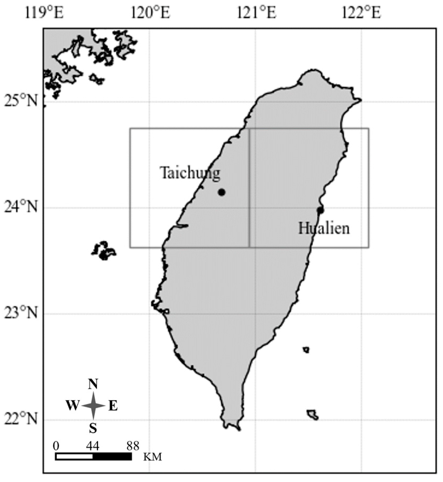
3.1. Case Area and Historical Rainfall

The rainfall data of the stations in Taichung and Hualien used in this study are from Taiwan’s Central Weather Administration (CWA) (https://www.cwa.gov.tw/V8/C/, accessed on December 2024). Their geographical locations are shown in Figure 3. Their longitude, latitude, altitude, and rainfall period used in this study are shown in

Table 1. Table of study cases.

Station	Station Code	Longitude	Latitude	Altitude (m)	Date
Taichung	467490	120°40′33.31″ E	24°08′50.98″ N	16	January 1950–December 2000
Hualien	466990	121°36′17.98″ E	23°58′37.10″ N	34	January 1950–December 2000

. Taichung and Hualien are located approximately 150 km apart on opposite sides of the Central Mountain Range, whose peaks reach around 4000 m. The rainfalls in these areas vary greatly. To coordinate with the historical scenario data of GCM, rainfall data from 1950 to 2005 used in this study are measured monthly.

3.2. GCM Data

According to IPCC AR5 (the current data for use are recommended by WRA), climate change caused by excessive anthropogenic greenhouse gas emissions will become increasingly apparent. By the end of the 21st century, the global surface temperature will rise by 1.5 to 2 degrees, and the difference between dry and wet seasons will become more significant. In AR5’s GCM model, the representative concentration pathways (RCPs) are used to define the severity of future climate change scenarios, and the radiative forcing (RF) is used as an indicator for differentiation. Kitoh et al. [1] used RCP 4.5 and RCP 8.5 scenarios to analyze global and regional monsoon rainfall changes. Majhi [35], with RCP 4.5 as a stable development scenario and RCP 8.5 as an adverse scenario, explored the influences of changes in future rainfall and temperature on the hydrologic cycle in India. The future scenarios employed in this study are RCP 4.5 and RCP 8.5. RF will change stably in RCP 4.5 by 2100, with an increase in 4.5 watts per square meter, indicating moderate greenhouse gas emissions. RF will increase in RCP 8.5 by 2100, with an increase in 8.5 watts per square meter, indicating high greenhouse gas emissions.

GCM data utilized in this study include historical and future data scenarios such as RCP 4.5 and RCP 8.5. The historical data covers the period from January 1950 to December 2005. The future scenarios are from January 2006 to December 2100. The data are measured in months. The IPCC website (https://www.ipcc-data.org/sim/gcm_monthly/AR5/, accessed on December 2024) shows future scenarios estimated by many research institutions worldwide using GCM in AR5 for researchers to download and use. This study selects two models, namely, ACCESS1.0 (ACCESS) and CSIRO-MK3.6.0 (CSMK3), from the assessment report issued by WRA as regional water resources assessment in 2016. Their horizontal grid resolutions are 192 (km) × 145 (km) and 192 (km) × 96 (km) with 19 and 12 factors, respectively. In AR5, GCM variable data are in netCDF4 (.nc) format.

In this study, the netCDF4 package of python is used to read variable data. After confirming variable names, it converts latitude and longitude into grids. After the confirmation that the selected latitude and longitude are converted into grids correctly, the data of 12 grids around the grid data of 4 selected stations in Taichung and Hualien are averaged. This avoids specific values of single grids [36]. The downscaling model is named as a combination of station name (C for Taichung and H for Hualien), GCM, and method of input variables (ORG for original variables and KPCA for data transformed by KPC). For example, C_ACCESS_ORG means that the DNN downscaling model is established with rainfall data of Taichung station, ACCESS model of GCM, and original data (ORG). The factors of AR5 used in this study include atmosphere, land, aerosol, and ocean, and the missing values are excluded. The final variables of GCM downscaling are shown in

Table 2. Table of atmospheric and oceanic factors for two GCM models.

Model	Factors	Factor Full Name
ACCESS and CSMK3	Atmosphere	Total Cloud Fraction
		Evaporation
		Specific Humidity
		Near-Surface Specific Humidity
		Precipitation
		Surface Air Pressure
		Sea Level Pressure
		Surface Net Downward Longwave Radiation
		Near-Surface Air Temperature
		Eastward Near-Surface Wind
		Northward Near-Surface Wind
	Aerosol Glue	Total Emission Rate of SO2
ACCESS	Ocean	Water Evaporation Flux Where Ice Free Ocean over Sea
		Northward Ocean Heat Transport
		Ocean Heat X Transport
		Ocean Heat Y Transport
		Rainfall Flux Where Ice Free Ocean over Sea
		Net Downward Shortwave Radiation at Sea Water Surface

.

4. Downscaling Model Construction

This study uses TensorFlow to build the DNN downscaling model. TensorFlow, an open-source deep learning framework developed by Google, is widely applied in fields such as machine learning, deep learning, natural language processing, and image recognition. It provides a powerful library for building neural network models. The core of TensorFlow is TensorFlow core library, which defines the essential components required for deep learning. In this study, the Keras module, a wrapper interface of TensorFlow, is used to construct the DNN downscaling model.

The steps for building the DNN downscaling model in this study are as follows.

(1)

Select input variables.

(2)

Determine DNN architecture, such as optimizers, activation functions, number of layers (NL), number of nodes per layer (NNPL).

(3)

DNN hyper-parameter optimization.

Step (1) is described in Section 4.1; steps (2) and (3) are explained in Section 4.2.

In this study, four performance assessment indicators (shown in Equations (7) and (8)), root mean square error (RMSE) and correlation coefficient (CC), are applied to assess the performance of the models. In Equations (7) and (8), $y_i$ is the observed value; $\overline{y}$ is the mean of the observed value; $y_i$ is the predicted value; $\overline{{\widehat{y}}_i}$ is the mean of the predicted value; and n is number of data items.

$$\mathrm{RMSE}=\sqrt{{\displaystyle \frac{\sum {\left(y_i{-\widehat{y}}_i\right)}^2}{n}}}$$

(7)

$$\mathrm{CC}={\displaystyle \frac{\sum _{i=1}^n(y_i-\overline{y})({\widehat{y}}_i-\overline{{\widehat{y}}_i})}{\sqrt{\sum _{i=1}^n{\left(y_i-\overline{y}\right)}^2}\sqrt{\sum _{i=1}^n{\left({\widehat{y}}_i-\overline{{\widehat{y}}_i}\right)}^2}}}$$

(8)

4.1. Predictive Variable Selection

In this study, original variables are selected, and KPCA is used for data conversion. Standardizing the data to z-scores helps eliminate the effect of differing scales across variables.

After standardizing variables, the model can iterate fast, the time of gradient descent can be reduced, and features between factors are preserved and scaled to improve the model accuracy. Based on the results of APS in this study, the optimal value of γ is 0.099 and 0.427 for Taichung and Hualien in ACCESS, and 0.082 and 0.667 for Taichung and Hualien in CSMK3, respectively.

After finding the optimal γ, it is used to convert original data into different radial basis functions with parameters (1 to 19 in ACCESS, 1 to 12 in CSMK3). Then, KPCs with the highest accuracy are selected as the final number by using KNN. The results of the number of KPCs and corresponding accuracy for Taichung and Hualien are shown in

Table 3. The accuracy of using KNN to determine the number of KPCs.

Station	GCM Model	Accuracy (%)	KPC
Taichung	Access	82.4	4
	CSMK3	78.6	5
Hualien	Access	81.3	13
	CSMK3	79.2	3

.

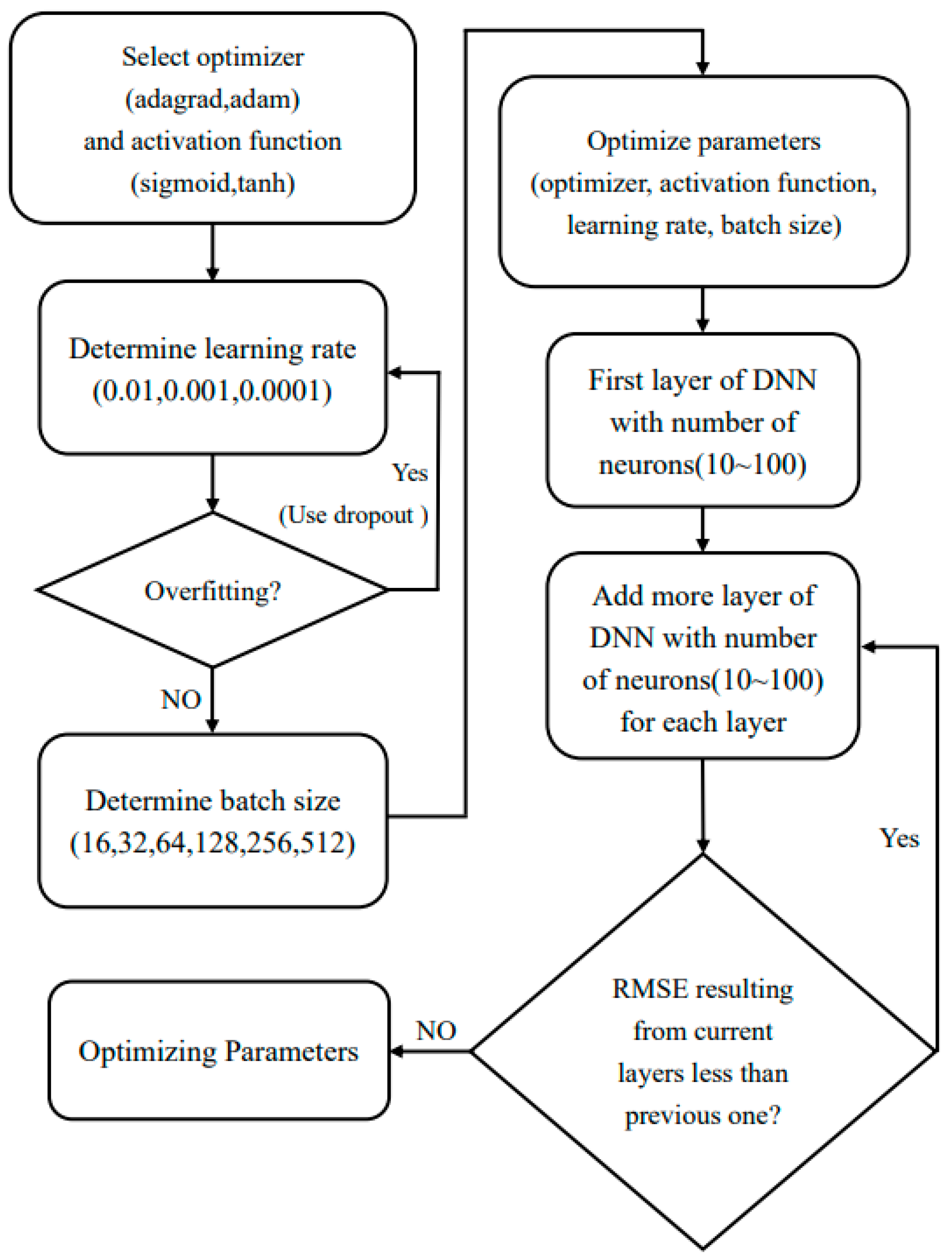
4.2. Model Parameter Optimization

It is highly time-consuming and difficult to determine DNN model architecture and optimize corresponding parameters. Therefore, both model architecture and parameter optimization must be considered. This study obtains the optimal solutions of DNN parameters according to the stage optimization proposed by Bai et al. [37,38]. The steps are shown below:

(1)

Determine the hidden layers.

This study follows the stage optimization approach proposed by Bai et al. [37,38] to obtain the optimal solutions for DNN parameters. According to Bengio [39], a minimum of 10,000 iterations is required for training. In our study, we have applied 50,000 iterations. Regarding the number of hidden layers, Liu [20] suggests that one to two hidden layers are ideal for optimization. Bai et al. [37,38] recommend using one to three hidden layers, with progressive optimization. Similarly, Busseti [40] proposes using two to three hidden layers for optimization, while Dalto [12] used three hidden layers and recommended the same number of layers for optimal performance.

Based on these findings, this study starts with one hidden layer and increases the number of hidden layers progressively during optimization.

(2)

Determine the number of nodes in the hidden layer.

Coppola Jr. et al. [41] suggested that if the input layer has n factors, there are 2n + 1 nodes in the hidden layer. Bai et al. [37] said that there is no mature method to determine the number of node layers in theory. There are 5 to 30 nodes in the hidden layer of our model. Busseti [40] used 10 to 50 nodes for training. In this study, the number of nodes to be measured ranges from 10 to 100.

Figure 4 shows the process of the preferred DNN downscaling model, divided into preferred optimizer, learning rate, batch size, and DNN architecture (number of hidden layers and number of neurons in each hidden layer). The initial architecture of the DNN model consists of one hidden layer, with the number of nodes in the hidden layer set within the range of 10 to 100. The number of hidden layers and the number of nodes are added based on performance evaluation metrics. Parameters to be optimized include optimizers, activation functions, batch size, NL, and NNPL. In this study, AdaGrad and Adam are the optimizers. The activation functions are sigmoid and tanh, with batch sizes of 16, 32, and 64. The number of nodes ranges from 10 to 100 at an interval of 5. The parameter optimization steps are as follows: (i) Determine the best optimizer, activation function, and learning rate. (ii) Determine the best batch size. (iii) Optimize the NL and NNPL.

The detailed process of determining the parameters of the DNN model is shown below:

i.

Optimizers and activation functions.

• The initial batch size is 16, the NL is 1, and the number of nodes is 10 and 50 to determine its convergence trend. Its learning rate is adjusted to converge. Optimizers and activation functions are selected to achieve convergence. After selecting optimizers and activation functions, learning rates are adjusted to determine overfitting. If there is overfitting, dropout will be performed on the DNN architecture. Finally, according to RMSE, AdaGrad is selected as the optimizer, and sigmoid is selected as the activation function. The learning rate is ${10}^{-3}$ and the batch size is optimized.

ii.

Batch size.

• The batch size is tested based on the selected optimizer, activation function, learning rate, and the setting of 1 DNN layer and 10 nodes. The batch size is changed from 16 to 512. After comparing RMSE, 64 is selected as the optimal batch size to optimize the number of node layers. First, it is assumed that DNN has 10 nodes per layer, with the number of nodes gradually increasing in units of 5 (10, 15, 20…, and 100). For in-order training, the number of nodes in the first layer is 85, which is the number of nodes at the minimum RMSE. After determining the number of nodes in the first layer, a second layer is added to the DNN architecture. The number of nodes in the second layer starts from 10 and gradually increases in units of 5. The number of nodes (35) at the minimum RMSE is taken as the number of nodes in the second layer. If the RMSE of the optimal number of nodes in the second layer is smaller than that of the optimal number of nodes in the first layer, a third layer will be added to DNN based on the above method. Otherwise, the DNN architecture is determined, and parameters are optimized.

iii.

NL and NNPL.

• The NL and NNPL are finally optimized to obtain optimal parameters. AdaGrad is selected as the optimizer, and sigmoid is selected as the activation function. The learning rate is ${10}^{-4}$ and the batch size is 64. The first layer has 100 nodes, and the second layer has 35 nodes. The final optimized parameters of GCM at all stations are shown in

  Table 4. Table of the optimization parameters in the DNN downscaling model.

  GCM	Station	Type	Quantity	Gamma	Optimizer	Activation Function	Learning Rate	Batch Size	Layer 1	Layer 2	Dimensionless RMSE
  ACCESS	Taichung	original	19	0.099	adagrad	sigmoid	0.0001	16	80		0.803
  		KPCA	4		adagrad	sigmoid	0.0041	64	100	35	0.835
  	Hualien	original	19	0.427	adagrad	sigmoid	0.001	64	55		1.007
  		KPCA	13		adagrad	sigmoid	0.0001	16	70		1.105
  CSMK3	Taichung	original	12	0.082	adagrad	sigmoid	0.001	64	40		0.845
  		KPCA	5		adagrad	sigmoid	0.001	32	10		1.593
  	Hualien	original	12	0.667	adagrad	tanh	0.01	16	90		1.038
  		KPCA	12		adam	tanh	0.001	16	10		1.191

  . Y and X in Equation (5) are standardized before calculation, and KPCA is noticeably larger in dimensionless RMSE (DR) of the ACCESS and CSMK3 models. Most optimizers are AdaGrad, and most activation functions are sigmoid. Learning rates mostly fall in between ${10}^{-2}$ and ${10}^{-3}$, and the batch sizes are 16, 32, or 64, usually with 1 layer.

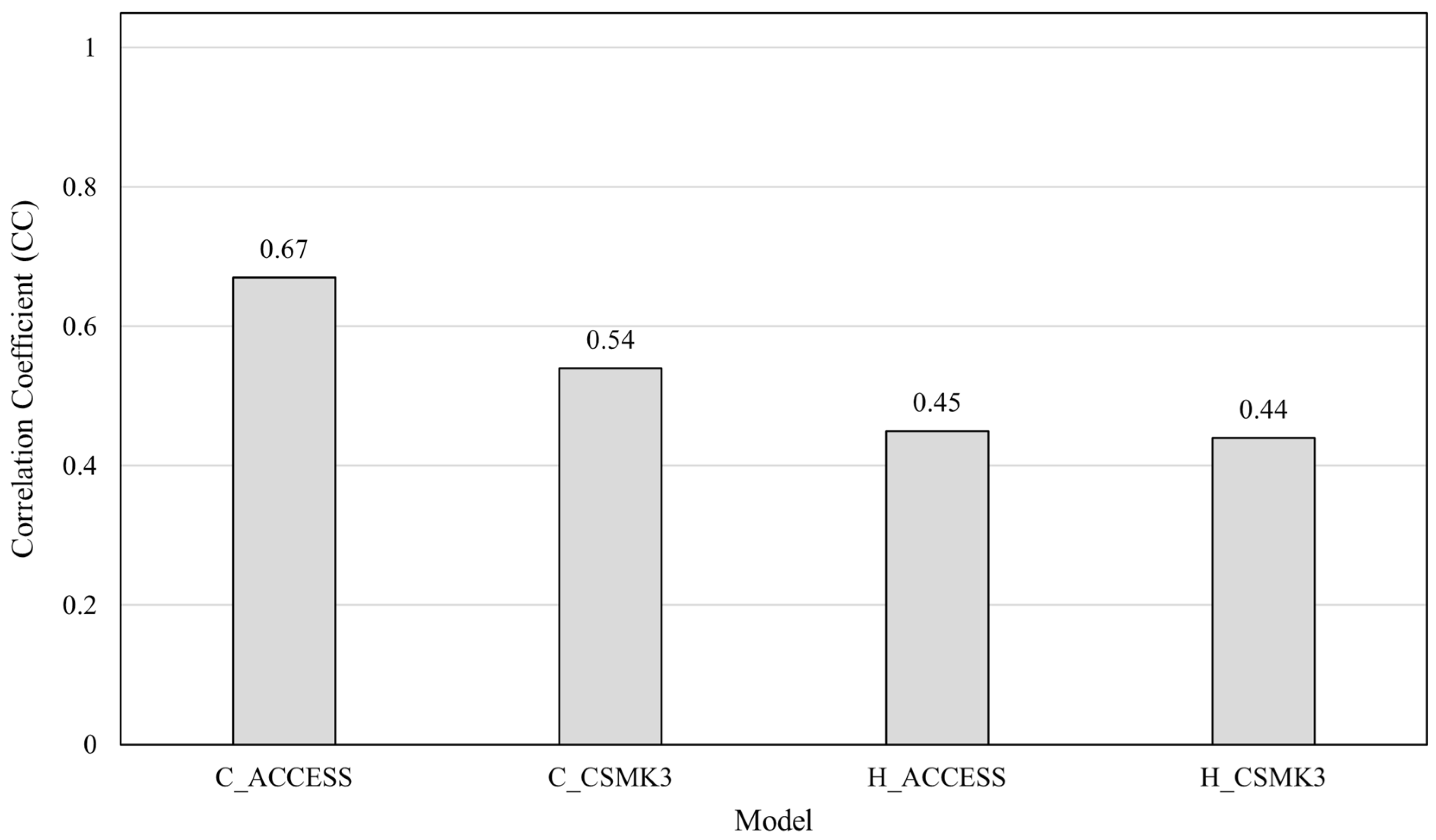
4.3. Assessment of the Effectiveness of Historical Scenarios

After the parameters of the above 4.2 DNN architecture are determined, a DNN statistical downscaling model is built based on the historical scenarios of ACCESS and CSMK3 and the historical records of Taichung and Hualien stations. The data period is from 1950 to 2005, and monthly rainfall and historical atmospheric and oceanic factors are used. There are a total of 672 data items/points. The data are ranked according to their number, and the data period is divided at a ratio of 3:1:1; training (January 1950 to December 1983); verification (January 1984 to December 1994); testing (January 1995 to December 2005).

Figure 5 shows the CC of the simulated results of different models (ACCESS and CSMK3) using test data for Taichung (C) and Hualien (H). Overall, the ACCESS model performs better than the CSMK3 model, and the CC of both models are higher in Taichung than those in Hualien. This is mainly because the ACCESS model considers both atmospheric and oceanic factors, while CSMK3 only considers atmospheric factors. It can better represent the characteristics of regional climate for Taiwan surrounded by the ocean, as both atmospheric and oceanic factors are contemplated.

5. Result and Discussion

Data from RCP 4.5 (moderate carbon emission) and RCP 8.5 (high carbon emission) are used for future scenarios. The aforementioned DNN model is used to predict future monthly rainfall based on future scenario factors (future scenario data from January 2006 to December 2100) to analyze rainfall trends and uncertainties in winter (December, January, February), summer (June, July, August), and in the future mid-term to long-term (mid-term: 2051 to 2060, long term: 2071 to 2080).

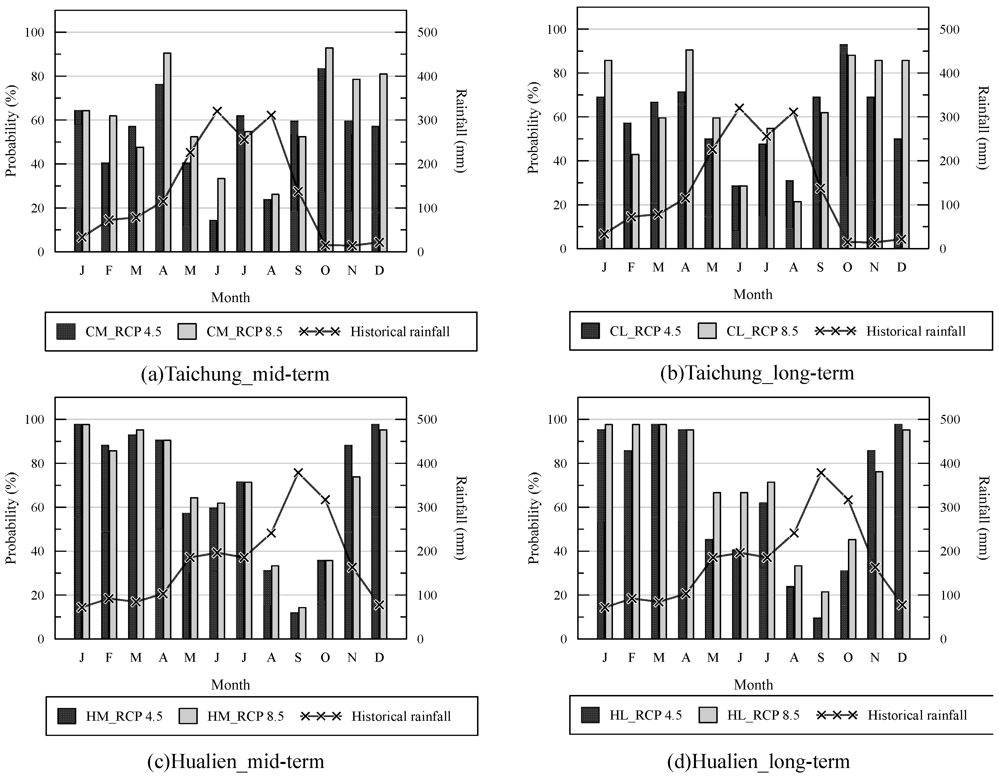
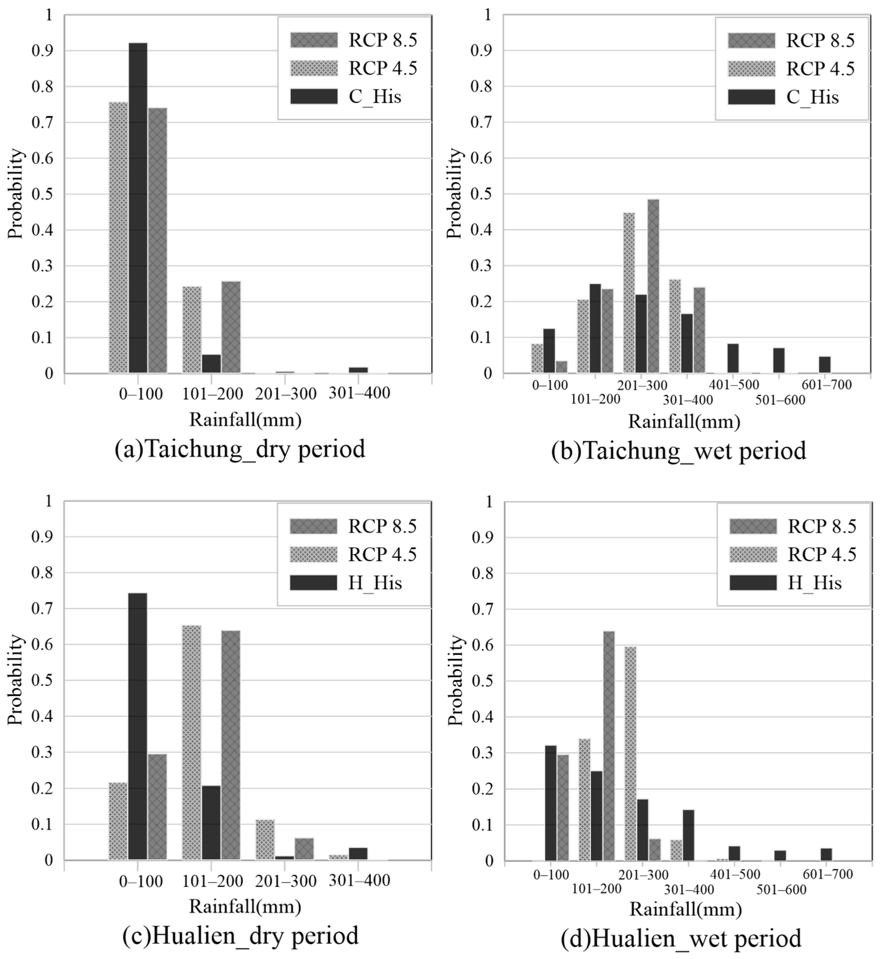
5.1. Statistical Probability Analysis of Rainfall in Future Scenarios

According to the rainfall classification of Taiwan’s Central Weather Bureau, the historical monthly rainfall is ranked in descending order, and the monthly rainfall marked 30% and 70% is selected. The rainfall is divided into three ranges: low rainfall below 30%, high rainfall above 70%, and normal rainfall in-between. For example, in Taichung, the predicted monthly rainfall of less than 24 (mm) is low, the predicted monthly rainfall between 24 (mm) and 157.9 (mm) is normal, and the predicted monthly rainfall of above 157.9 (mm) is high. The analysis of the three-class classification is shown in Figure 6. The annual rainfall is divided into the wet season (May–October) and the dry season (November–April of the next year). Regardless of mid-term to long-term or emission scenarios, the probability of future dry season rainfall exceeding the upper limit of normal is over 50% in Taichung and over 90% in Hualien. This indicates a high probability that the future dry season rainfall exceeds the upper limit of the historical normal and an increase in future dry season rainfall.

In the wet season, regardless of emission scenarios, the probability that rainfall within the historically normal range in the mid-term to long-term is higher than 50% in Taichung and higher than 70% in Hualien. This indicates a high probability that the future wet season rainfall is within the historically normal range. It is worth noting that Taichung has a nearly 50% probability of rainfall below the lower limit of the historical normal, while Hualien shows an extremely low probability of rainfall below the historically normal range. The probability of reduced rainfall in Hualien in the future is extremely low. Throughout the year, the trend is roughly similar to the wet season.

Figure 7 compares the probability of monthly precipitation exceeding historical average values for Taichung and Hualien under different emission scenarios in the medium-term to long-term future. The dark and light bars represent the probabilities for RCP 4.5 and RCP 8.5 scenarios, respectively, while the line graph shows the historical average monthly precipitation. According to the chart, in any scenario in the future mid-term and long-term, the monthly rainfall in Taichung in winter and spring (namely, the dry season) exceeds the historical average by more than 60%. The exceeded probability of 80% in the RCP 8.5 scenario from October to January indicates a high probability that the future dry season rainfall will increase in Taichung. In comparison, the rainfall from June to August (summer, the main rainfall period in the wet season) exceeds the historical average by less than 50%. In particular, the exceeding probability in June and August is close to 20%, and the probability in RCP 4.5 is significantly lower. This indicates that the trend of wet season rainfall decrease in Taichung will increase in future scenarios. In Hualien, the probability of monthly rainfall exceeding the historical average is less than 40% from August to October, and monthly rainfall exceeding the historical average is more than 60% in all other months. This indicates a high probability that the dry season rainfall will increase in Hualien in the mid-term and long-term regardless of future scenarios. In terms of scenarios in Taichung, the probability of dry season rainfall exceeding the historical average in RCP 8.5 is higher than that in RCP 4.5, which is not obvious in the wet season. In Hualien, RCP 4.5 and RCP 8.5 have roughly equal probability of above-average rainfall in the mid-term, while RCP 8.5 is higher than RCP 4.5 in the long-term. The above results indicate that under the RCP 8.5 scenario, there is a high likelihood of increased precipitation during the dry season in Taichung and Hualien, while a decreasing trend in rainfall during the wet season is observed. Hualien shows a higher likelihood in both seasons. Due to Taiwan’s eastern region being close to the western Pacific and influenced by the Central Mountain Range, the impact of climate change on the temporal distribution of rainfall in the eastern part of the Central Mountain Range is expected to be more significant in the future.

Figure 8 shows the distribution of historical and predicted precipitation for Taichung and Hualien under the RCP 4.5 and RCP 8.5 scenarios, across different ranges. The figure shows that Taichung’s historical and future rainfall is mainly between 0 mm and 100 mm in the dry season, with a probability higher than 0.7. However, the probability of future rainfall in this range will reduce. In Taichung, the wet season rainfall mainly ranges from 101 mm to 200 mm, 201 mm to 300 mm, and 301 mm to 400 mm. The probability of future rainfall increase is high, and the rainfall in RCP 8.5 is higher than in RCP 4.5. The dry season rainfall ranges from 0 mm to 100 mm, showing a decreasing trend, and the rainfall from 101 mm to 200 mm shows an increasing trend. In Hualien, the rainfall increases sharply within the range of 101 mm to 200 mm in the dry season and 101 mm to 300 mm in the wet season. In terms of variability of the future rainfall range, the wet season rainfall in Hualien ranges from 201 mm to 300 mm, with the highest variability and RCP 4.5 much higher than RCP 8.5. The results indicate that precipitation variability is increasing, highlighting the water resources for early adaptation, especially in western Taiwan.

5.2. Mid-Term and Long-Term Rainfall Assessment in Future Scenarios

In this study, by using GCM models with future scenarios, the percentage increase and decrease of monthly rainfall and historical average rainfall calculated are drawn into a box plot, as shown in Figure 9. The figure shows the box plot of percentage increase and decrease of monthly rainfall and historical average monthly rainfall in RCP 4.5 and RCP 8.5 for 12 months in Taichung and Hualien over the mid-term to long-term. The broken and dotted lines are the median percentage increase and decrease of monthly rainfall in RCP 8.5 and RCP 4.5, respectively. As shown in Figure 8, the rainfall during the wet season exhibits a decreasing trend with lower variability and uncertainty. In contrast, the rainfall during the dry season shows an increasing trend, but with higher variability and greater uncertainty. This indicates that the wet season rainfall will be severely affected. In contrast, the future dry season rainfall increases in Taichung and Hualien have high variability. This indicates that the uncertainty increases, although there is an increasing trend. Overall, in RCP 4.5 and RCP 8.5, the percentage increase and decrease of monthly rainfall changes are similar in Taichung and Hualien. Future water resource policies must be adjusted to address the impacts on potential increases in dry season rainfall and decreases in wet season rainfall.

6. Conclusions

This study employs KPCA and DNN downscaling models to assess the trends and uncertainties of future monthly rainfall in Taichung and Hualien of Taiwan. Historical monthly rainfall and GCM future scenario data (RCP 4.5 and RCP 8.5) are used to estimate future rainfall. The following conclusions are drawn based on the simulation results:

1.

In DNN models, AdaGrad is a better optimizer, sigmoid is a better activation function, and one hidden layer is more appropriate.

2.

The ACCESS GCM model considering both atmospheric and oceanic factors performs better for Taiwan.

3.

According to the analysis of the three-class rainfall classification in future scenarios, Taichung and Hualien have a high probability of future dry season rainfall exceeding the upper limit of historical normal. There is a high probability that future wet season rainfall will fall in the normal range of historical rainfall.

4.

The dry season rainfall in Taichung and Hualien shows an increasing trend, but with higher variability and uncertainty. The wet season rainfall decreases significantly, but with lower variability, indicating that the uncertainty in the decreasing trend is smaller.

5.

The probability of future dry season rainfall exceeding historical averages in Taichung and Hualien is greater than 60%, indicating a higher likelihood of increased rainfall. The probability of future wet season rainfall exceeding historical averages in Taichung and Hualien is lower than 50%, indicating a greater likelihood of reduced rainfall.

6.

Under the RCP 8.5 scenario, the impacts on rainfall increase in the dry season and rainfall decrease in the wet season are more pronounced compared to RCP 4.5. This suggests that climate change has a greater impact on the spatio-temporal distribution of rainfall, and early adaptation strategies should be implemented.

7. Limitations and Future Work

This study uses the GCM models from CMIP 5 as recommended by Water Resources Agency (WRA) of the Ministry of Economic Affairs, Taiwan, for future water resource assessments, while considering the climatic differences affected by the Central Mountain Range at the same latitude. Further exploration is still needed on other aspects. Future research will employ the CMIP 6 data to investigate the impacts and compare the differences.

References

1. Kitoh, A.; Endo, H.; Krishna Kumar, K.; Cavalcanti, I.F.; Goswami, P.; Zhou, T. Monsoons in a Changing World: A Regional Perspective in a Global Context. J. Geophys. Res. Atmos. 2013, 118, 3053–3065. [Google Scholar] [CrossRef]
2. Manor, A.; Berkovic, S. Bayesian Inference Aided Analog Downscaling for Near-Surface Winds in Complex Terrain. Atmos. Res. 2015, 164, 27–36. [Google Scholar] [CrossRef]
3. Salvi, K.; Ghosh, S. High-Resolution Multisite Daily Rainfall Projections in India with Statistical Downscaling for Climate Change Impacts Assessment. J. Geophys. Res. Atmos. 2013, 118, 3557–3578. [Google Scholar] [CrossRef]
4. Al-Mukhtar, M.; Qasim, M. Future Predictions of Precipitation and Temperature in Iraq Using the Statistical Downscaling Model. Arab. J. Geosci. 2019, 12, 25. [Google Scholar] [CrossRef]
5. Baghanam, A.H.; Eslahi, M.; Sheikhbabaei, A.; Seifi, A.J. Assessing the Impact of Climate Change over the Northwest of Iran: An Overview of Statistical Downscaling Methods. Theor. Appl. Climatol. 2020, 141, 1135–1150. [Google Scholar] [CrossRef]
6. Xu, Z.; Han, Y.; Yang, Z. Dynamical Downscaling of Regional Climate: A Review of Methods and Limitations. Sci. China Earth Sci. 2019, 62, 365–375. [Google Scholar] [CrossRef]
7. Zhang, H.; Singh, V.P.; Wang, B.; Yu, Y. CEREF: A Hybrid Data-Driven Model for Forecasting Annual Streamflow from a Socio-Hydrological System. J. Hydrol. 2016, 540, 246–256. [Google Scholar] [CrossRef]
8. Kundu, S.; Khare, D.; Mondal, A. Future Changes in Rainfall, Temperature, and Reference Evapotranspiration in Central India by Least Square Support Vector Machine. Geosci. Front. 2017, 8, 583–596. [Google Scholar] [CrossRef]
9. Li, C.Y.; Lin, S.S.; Chuang, C.M.; Hu, Y.L. Assessing Future Rainfall Uncertainties of Climate Change in Taiwan with a Bootstrapped Neural Network-Based Downscaling Model. Water Environ. J. 2020, 34, 77–92. [Google Scholar] [CrossRef]
10. Sulaiman, N.A.; Shaharudin, S.M.; Zainuddin, N.H.; Najib, S.A. Improving Support Vector Machine Rainfall Classification Accuracy Based on Kernel Parameters Optimization for Statistical Downscaling Approach. Int. J. 2020, 9, 652–657. [Google Scholar] [CrossRef]
11. Vidyarthi, V.K.; Jain, A. Advanced Rule-Based System for Rainfall Occurrence Forecasting by Integrating Machine Learning Techniques. J. Water Resour. Plan. Manage. 2023, 149, 04022072. [Google Scholar] [CrossRef]
12. Dalto, M.; Matuško, J.; Vašak, M. Deep Learning Neural Networks for Ultra-Short-Term Wind Forecasting. In Proceedings of the 2015 IEEE International Conference on Industrial Technology (ICIT), Seville, Spain, 17–19 March 2015; pp. 1657–1663. [Google Scholar] [CrossRef]
13. Wang, Y.; Basu, S. Using an artificial neural network approach to estimate surface-layer optical turbulence at Mauna Loa, Hawaii. Opt. Lett. 2016, 41, 2334–2337. [Google Scholar] [CrossRef] [PubMed]
14. Bi, C.; Qing, C.; Wu, P.; Jin, X.; Liu, Q.; Qian, X.; Zhu, W.; Weng, N. Optical turbulence profile in marine environment with artificial neural network model. Remote Sens. 2022, 14, 2267. [Google Scholar] [CrossRef]
15. Frame, J.M.; Kratzert, F.; Klotz, D.; Gauch, M.; Shalev, G.; Gilon, O.; Qualls, L.M.; Gupta, H.V.; Nearing, G.S. Deep Learning Rainfall–Runoff Predictions of Extreme Events. Hydrol. Earth Syst. Sci. 2022, 26, 3377–3392. [Google Scholar] [CrossRef]
16. Shikhovtsev, A.Y.; Kovadlo, P.G.; Kiselev, A.V.; Eselevich, M.V.; Lukin, V.P. Application of Neural Networks to Estimation and Prediction of Seeing at the Large Solar Telescope Site. Publ. Astron. Soc. Pac. 2023, 135, 014503. [Google Scholar] [CrossRef]
17. Aswin, S.; Geetha, P.; Vinayakumar, R. Deep Learning Models for the Prediction of Rainfall. In Proceedings of the 2018 International Conference on Communication and Signal Processing (ICCSP), Chennai, India, 3–5 April 2018; pp. 657–661. [Google Scholar] [CrossRef]
18. Yen, M.H.; Liu, D.W.; Hsin, Y.C.; Lin, C.E.; Chen, C.C. Application of the Deep Learning for the Prediction of Rainfall in Southern Taiwan. Sci. Rep. 2019, 9, 12774. [Google Scholar] [CrossRef] [PubMed]
19. Basha, C.Z.; Bhavana, N.; Bhavya, P.; Sowmya, V. Rainfall Prediction Using Machine Learning & Deep Learning Techniques. In Proceedings of the 2020 International Conference on Electronics and Sustainable Communication Systems (ICESC), Coimbatore, India, 2–4 July 2020; pp. 92–97. [Google Scholar] [CrossRef]
20. Liu, F.; Xu, F.; Yang, S. A Flood Forecasting Model Based on Deep Learning Algorithm via Integrating Stacked Autoencoders with BP Neural Network. In Proceedings of the 2017 IEEE Third International Conference on Multimedia Big Data (BigMM), Laguna Hills, CA, USA, 19–21 April 2017; pp. 58–61. [Google Scholar] [CrossRef]
21. Xiang, Y.; Gou, L.; He, L.; Xia, S.; Wang, W. A SVR–ANN Combined Model Based on Ensemble EMD for Rainfall Prediction. Appl. Soft Comput. 2018, 73, 874–883. [Google Scholar] [CrossRef]
22. Lin, S.S.; Hu, Y.L.; Zhu, K.Y. Downscaling Model for Rainfall Based on the Influence of Typhoon under Climate Change. J. Water Clim. Change. 2022, 13, 2443–2458. [Google Scholar] [CrossRef]
23. Pulkkinen, S. Nonlinear Kernel Density Principal Component Analysis with Application to Climate Data. Stat. Comput. 2016, 26, 471–492. [Google Scholar] [CrossRef]
24. Hu, J.N.; Lin, S.S.; Zhu, K.Y. Integrating Nonlinear Principal Component Analysis and Neural Networks to Develop a Downscaling Model Evaluating Future Rainfall of Taichung and Hualien. J. Taiwan Agric. Eng. 2020, 67, 78–90. [Google Scholar] [CrossRef]
25. Hawkins, D.M. The Problem of Overfitting. J. Chem. Inf. Comput. Sci. 2004, 44, 1–12. [Google Scholar] [CrossRef]
26. Fischer, A.; Bunke, H. Kernel PCA for HMM-Based Cursive Handwriting Recognition. In Proceedings of the International Conference on Computer Analysis of Images and Patterns, Münster, Germany, 2–4 September 2009; Springer: Berlin, Heidelberg, 2009; pp. 181–188. [Google Scholar] [CrossRef]
27. Debruyne, M. Detecting Influential Observations in Kernel PCA. Comput. Stat. Data Anal. 2010, 54, 3007–3019. [Google Scholar] [CrossRef]
28. Jiang, M.; Zhu, L.; Wang, Y.; Xia, L.; Shou, G.; Liu, F.; Crozier, S. Application of Kernel Principal Component Analysis and Support Vector Regression for Reconstruction of Cardiac Transmembrane Potentials. Phys. Med. Biol. 2011, 56, 1727. [Google Scholar] [CrossRef] [PubMed]
29. Alam, M.A.; Fukumizu, K. Hyperparameter selection in kernel principal component analysis. J. Comput. Sci. 2014, 10, 1139. [Google Scholar] [CrossRef]
30. Kaneko, H. k-Nearest Neighbor Normalized Error for Visualization and Reconstruction—A New Measure for Data Visualization Performance. Chemom. Intell. Lab. Syst. 2018, 176, 22–33. [Google Scholar] [CrossRef]
31. Ezukwoke, K.; Zareian, S.J. Kernel Methods for Principal Component Analysis (PCA): A Comparative Study of Classical and Kernel PCA. A Prepr. 2019. [Google Scholar] [CrossRef]
32. Li, C.H.; Lin, C.T.; Kuo, B.C.; Ho, H.H. An Automatic Method for Selecting the Parameter of the Normalized Kernel Function to Support Vector Machines. In Proceedings of the 2010 International Conference on Technologies and Applications of Artificial Intelligence, Hsinchu, Taiwan, 18–20 November 2010; pp. 226–232. [Google Scholar] [CrossRef]
33. Li, C.H.; Hsien, P.J.; Lin, L.H. A Fast and Automatic Kernel-Based Classification Scheme: GDA+SVM or KNWFE+SVM. J. Inf. Sci. Eng. 2018, 34, 1–12. [Google Scholar] [CrossRef]
34. Fix, E.; Hodges, J.L. Discriminatory Analysis. Nonparametric Discrimination: Consistency Properties. Int. Stat. Rev. 1989, 57, 238–247. [Google Scholar] [CrossRef]
35. Majhi, S.; Pattnayak, K.C.; Pattnayak, R. Projections of Rainfall and Surface Temperature over Nabarangpur District Using Multiple CMIP5 Models in RCP 4.5 and 8.5 Scenarios. Int. J. Appl. Res. 2016, 2, 399–405. [Google Scholar]
36. Beecham, S.; Rashid, M.; Chowdhury, R.K. Statistical Downscaling of Multi-Site Daily Rainfall in a South Australian Catchment Using a Generalized Linear Model. Int. J. Climatol. 2014, 34, 3654–3670. [Google Scholar] [CrossRef]
37. Bai, Y.; Chen, Z.; Xie, J.; Li, C. Daily Reservoir Inflow Forecasting Using Multiscale Deep Feature Learning with Hybrid Models. J. Hydrol. 2016, 532, 193–206. [Google Scholar] [CrossRef]
38. Bai, Y.; Sun, Z.; Zeng, B.; Deng, J.; Li, C. A Multi-Pattern Deep Fusion Model for Short-Term Bus Passenger Flow Forecasting. Appl. Soft Comput. 2017, 58, 669–680. [Google Scholar] [CrossRef]
39. Bengio, Y. Practical Recommendations for Gradient-Based Training of Deep Architectures. In Neural Networks: Tricks of the Trade; Springer: Berlin/Heidelberg, Germany, 2012; pp. 437–478. [Google Scholar]
40. Busseti, E. Deep Learning for Time Series Modeling. In Technical Report; Stanford University: Stanford, CA, USA, 2012; pp. 1–5. [Google Scholar]
41. Coppola, E.A., Jr.; Rana, A.J.; Poulton, M.M.; Szidarovszky, F.; Uhl, V.W. A Neural Network Model for Predicting Aquifer Water Level Elevations. Groundwater 2005, 43, 231–241. [Google Scholar] [CrossRef] [PubMed]
Figure 1. Architecture of a deep neural network.
Atmosphere 16 00165 g001
Figure 2. Dropout conceptual scheme.
Atmosphere 16 00165 g002
Figure 3. Locations of the study of Taichung and Hualien.
Atmosphere 16 00165 g003
Figure 4. Flow chart of optimal parameters for optimizing DNN downscaling model.
Atmosphere 16 00165 g004
Figure 5. CC of ACCESS and CSMK3 downscaling models in Taichung and Hualien.
Atmosphere 16 00165 g005
Figure 6. Results of three classifications of the predicted precipitation in Taichung and Hualien. The downscaling model is named as station (C and H for Taichung and Hualien, respectively) + medium (M)/long (L)-term_RCP 4.5/8.5. CM_RCP 4.5 indicates medium-term rainfall model for Taichung using the RCP4.5 scenario.
Atmosphere 16 00165 g006
Figure 7. Comparison of the probability of the monthly rainfall and historical average monthly rainfall between Taichung and Hualien in different long-term emission scenarios in the future.
Atmosphere 16 00165 g007
Figure 8. The probability of the historical rainfall in wet period and dry period in Taichung and Hualien with different rainfall intervals in different scenarios in the future.
Atmosphere 16 00165 g008
Figure 9. Box plots of the percentage in the estimated monthly rainfall and historical average rainfall in the future scenarios of the two GCM models for RCP 4.5 and RCP 8.5.
Atmosphere 16 00165 g009