Abstract
Contrails form as a result of water vapor bonding with soot emitted from jet engines at cruise altitudes, leading to contrail formation in Ice Supersaturated Regions (ISSRs). Contrails are estimated to contribute approximately 2% to total anthropogenic global warming. Some researchers have developed simulation models to estimate the frequency, duration, and spatial distribution of contrails. Other researchers have identified issues with the accuracy of the data for predicting the timing and precise geographic positioning of ISSRs. This study presents a systematic review of 22 peer-reviewed articles that included detailed models of ISSR identification, identifying three atmospheric data sources, four parameters, and two equations for calculating the parameters derived. A further analysis revealed differences in the temperature and RHW readings across the three databases, resulting in differences in the RHI calculations and the identification of ISSRs. Over an 18-month period in Sterling, Virginia, USA, the radiosonde data and two atmospheric forecast databases identified the ISSR conditions on 44%, 47%, and 77% of days, respectively. Broken down by a flight level between 30,000 and 39,999 feet in altitude, these differences are highlighted further. The forecast databases overestimated the presence of ISSRs compared to the radiosonde data. These findings underscore the variability inherent in atmospheric datasets and the conversion methods, highlighting potential areas for refinement in ISSR prediction, notably in the development of ensemble forecasts based on several atmospheric databases. The implications of these results, the limitations of this study, and future work are discussed.
1. Introduction
Contrails, high-altitude cirrus-like clouds, are formed when water vapor and soot, emitted at high temperatures from jet engines into very cold air in cruise flight, bond to form ice crystals [1]. When the air temperature is specifically less than or equal to −41.1 °C (−41.98 °F) and its relative humidity with respect to ice is at least 100%, a contrail will form and persist [2].
Atmospheric regions, typically the upper troposphere, in which the conditions for contrail formation and persistence are met are known as Ice Supersaturated Regions (ISSR). ISSRs have been found to occur up to 30% of the time in cloud-free air masses over the North Atlantic [3] and 44% of the time in the airspace over Washington D.C. [4].
Contrails contribute to global warming via interference with the Earth’s natural radiation budget. At night, contrails absorb outgoing thermal long-wave radiation (33%) that would otherwise go out to space and have a warming effect [5]. During daylight, contrails reflect the incoming shortwave solar radiation (23%) back out into space, resulting in a cooling effect. The total impact is overwhelmingly warming, especially as most long-haul flights are flown at night. With longer cruise phases, there is a higher potential for flight through an ISSR, for contrail formation, and for longer contrails to form and a higher global warming potential [6]. In this way, contrails are the aviation sector’s largest contributor to the global climate impact, estimated at 2% of total anthropogenic global warming [7]. It should be noted that the impact of contrails surpasses that of direct carbon dioxide emissions when calculated using a 20-year equivalent carbon dioxide global warming potential time horizon (GWP20) [7]. Governmental bodies such as the National Aeronautics and Space Administration and industry partners such as GE Aerospace are prioritizing the study of contrails due to their impact on global warming [8].
The most effective, rapid, and lowest-cost method for reducing the number of contrails is rerouting individual flights vertically over or under ISSRs [9]. The feasibility and impact of this “navigational avoidance” approach has been evaluated in several studies [6,10,11,12,13,14,15]. The efficacy of this approach is predicated on the accurate identifications of ISSRs in the zones of the atmosphere used by airlines and aircraft operators.
This paper describes a systematic review of 22 peer-reviewed papers that describe the results of simulation models and flight planning tools to identify the occurrence, location, timing, and impact of contrails (and contrail avoidance).
This study identified three different sources of atmospheric data that were commonly used: the National Oceanic and Atmospheric Administration (NOAA) Rapid Refresh (RAP), the European Centre for Medium-Range Weather Forecasts Reanalysis (ECMWF/ERA5), and the Integrated Global Radiosonde Archive (IGRA). Whereas NOAA and ECMWF are physics-based atmospheric forecasts, IGRA is a global dataset of radiosonde (weather balloon) observations. IGRA includes atmospheric profiles of temperature, humidity, and wind from stations around the world.
Three parameters were used across all of the studies: temperature, pressure, and relative humidity to water (RHW). A critical step in the analyses is the conversion of RHW into relative humidity to ice (RHI). This conversion is conducted using the Goff–Gratch equations [16]. These parameters were selected as they are requisite to calculations of the Schmidt–Appleman criterion.
Discrepancies across the values of the parameters in the atmospheric forecast databases are present. Using the radiosonde data at a specified geographic location as a baseline, the temperature discrepancies across the flight levels averaged −4.5 °F and 2.4 °F across two different atmospheric databases. For relative humidity to water (RHW), the deviations averaged 6.6% and 24.8% across the same flight levels when compared to the radiosonde reference data.
Furthermore, over an 18-month period at the same geographic location, the radiosonde data and the two atmospheric forecast databases identified ISS conditions on 44%, 47%, and 77% of the days, respectively. The forecast databases overestimated ISSRs compared to the radiosonde data. These findings underscore the variability inherent in atmospheric datasets and conversion methods, highlighting potential areas for refinement in ISSR prediction.
There are three types of contrails: (1) short-lived contrails, (2) long-lived persistent contrails, and (3) long-lived contrail cirri (Figure 1). Short-lived contrails are line-shaped and have a duration of less than 10 min (Table 1). Persistent and contrail cirri have durations of up to 10 h and are often formed during long-haul flights, such as trans-continental and trans-oceanic flights. Persistent contrails remain line-shaped and can be as long as 10 km. Over time, due to non-uniform winds, turbulent (random) motion, and humidity fluctuations, persistent contrails lose their initial linear shape and transition into contrail cirri with irregular shapes. These contrails can overlap and merge with other contrails in traffic-congested areas, forming extended ice cloud layers with non-uniform shapes, depths, and durations. Persistent contrails may also merge with or form in natural cirri [17]. Irregular-shaped contrail cirri cannot be distinguished easily from natural cirri, hampering their observation. Contrails can also be transported considerable distances (e.g., 100 km) away from their location of generation, resulting in the presence of contrails in locations where ISS conditions are not met [4].
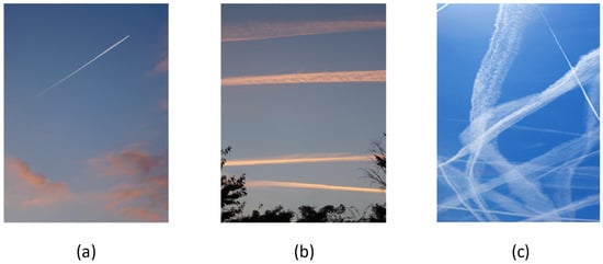
Figure 1.
Contrails: short-lived contrail (a), long-lived persistent contrails (b), and long-lived contrail cirrus (c).

Table 1.
Characteristics of contrails.
The formation and persistence of contrails, as well as their evolution into contrail cirri, depends on the relationship between temperature, relative humidity with respect to water (RHW), and relative humidity with respect to ice (RHI) (Table 2).
Table 2.
Delineations of the three classes of contrails.
Short-lived contrails form when the hot exhaust gases emitted by jet engines mix with the cold, ambient air, quickly cooling and condensing water vapor into ice crystals. According to the Schmidt–Appleman criterion (SAC), these short-lived contrails appear if the ambient air is cold enough and sufficiently humid, even if it is not supersaturated with respect to ice [18,19].
For persistent contrails and contrail cirri, the ambient conditions must meet additional criteria beyond the SAC, particularly the presence of ISSRs where the RHI exceeds 100% but the RHW can remain below saturation (RHW < 100%).
In ISSRs, the air contains more water vapor than ice would typically hold in equilibrium, allowing ice crystals from the contrails to grow and persist over longer timescales. This sustained supersaturation supports the transformation of contrails into long-lived contrail cirrus clouds.
The distinction between RHW and RHI is essential because while short-lived contrails only require a RHW near 100% for initial formation, the longevity and spread of contrail cirri depend on the maintenance of supersaturation with respect to ice.
The objectives of this paper are to identify the differences in parameters in the atmospheric forecasts used for ISSRs, quantify the differences in atmospheric condition forecasts, and quantify the differences in the identification of ISSRs.
This paper is organized as follows: Section 2 provides an overview of the materials and methods of analysis. Section 3 describes the results of the analysis. Section 4 discusses comparisons of temperature and relative humidity in forecasts of upper tropospheric ice supersaturation. Section 5 provides conclusions, implications, limitations, and suggestions for future work.
2. Materials and Methods
Peer-reviewed journal articles were identified for topics related to simulation modeling and/or flight trails related to navigational avoidance of Ice Supersaturated Regions. Searches were conducted in the Google Scholar and ProQuest databases using the terms “aircraft-induced clouds”, “climate forcing”, “energy forcing”, “forecast”, “humidity”, “ice supersaturation”, “radiative forcing”, “relative humidity”, “relative humidity with respect to ice”, “relative humidity with respect to water”, “Schmidt-Appleman Criteria”, and “supersaturation”. The resulting papers were inspected to ensure they satisfied the intent of the search and focused on ice supersaturation, specifically in terms of the study of contrails. Additional papers were identified through the references in these papers on the topic. The papers were required to provide details of the simulation models or tools (e.g., flight planning) and methods used to identify ISSRs—specifically, the source of the atmospheric data;, the parameters used to identify ISSRs, such as the Schmidt–Appleman criterion; and the equations used to calculate any of the derived parameters.
A quantitative analysis was conducted to compare the identification of ISSRs across the atmospheric databases IGRA, RAP, and ERA5 across the pressure altitude range shown in Table 3, covering the airspace over Sterling, Virginia, USA.
Table 3.
Parameters of data collection.
Simple linear interpolation (Equation (1)) was used to fill the gaps for 1000-foot increments in the ERA5 and RAP databases, where (x1, y1) and (x2, y2) were the existing data points, x was the altitude, and y was the estimated value at x. While temperature follows consistent patterns throughout the atmosphere, as identified in the International Standard Atmosphere, relative humidity does not follow any such pattern and is more difficult to forecast. The authors recognize that using linear interpolation for relative humidity is an oversimplification because linear interpolation of the atmospheric state parameters does not follow smooth functions. However, it is the most appropriate equation to use in this scenario.
3. Results
Twenty-two (22) papers were identified as meeting the criteria above. These papers were used to identify the following:
- The sources of atmospheric data (Section 4.1);
- The atmospheric parameters used (Section 4.2);
- Equations used for the derived atmospheric data (Section 4.3);
- Thresholds for the SAC and ISSR conditions (Section 4.4).
3.1. Sources of Atmospheric Data
A survey of twenty-two scientific papers identified six primary atmospheric databases used (Table 4). The first three databases in Table 4 are the most common and are thus compared in this study.
The majority of the publications on contrail-related research come from and focus on Europe (e.g., Germany, the Netherlands, Ireland, and France) and the United States. As such, the most commonly used databases as identified in the data sources from the literature review are the ECMWF ERA5, HRES, and IFS products, followed by NOAA-RAP and IGRA. Some of the databases were country-specific and thus inapplicable to this study, such as the DWD WAWFOR.
NOAA’s Rapid Refresh (RAP) system is an hourly updated, short-range weather prediction model, primarily focusing on the North American region. RAP leverages the Advanced Research Weather Research and Forecasting Model (WRF-ARW) and uses a 13 km horizontal resolution with 50 vertical layers. It is designed to provide high-frequency forecasts for up to 51 h for select cycles, making it particularly beneficial for aviation, severe weather, and renewable energy applications.
RAP gathers atmospheric data from a combination of sources: surface observations, aircraft data, satellite-derived information, radar observations, and soundings. Data assimilation incorporates these inputs to initialize the forecasts of the Advanced Research Weather Research Forecasting Model, optimizing the predictions by integrating real-time observations. The Gridpoint Statistical Interpolation (GSI) analysis method used in RAP significantly improves its cloud and precipitation predictions by incorporating hydrometeor and cloud data.
RAP is complemented by the High-Resolution Rapid Refresh (HRRR), a 3 km model focused on finer-scale convective events. Both RAP and HRRR are part of NOAA’s efforts to provide detailed, rapid updates to support operations requiring timely weather guidance [20].
The European Centre for Medium-Range Weather Forecasts (ECMWF) provides several weather and climate data products. ERA5 is the fifth-generation ECMWF reanalysis dataset, which reconstructs global climate data going back to 1950 and is updated with recent information. It provides hourly estimates of various atmospheric, oceanic, and land variables at a spatial resolution of about 31 km, making it a valuable tool for climate research, historical weather analysis, and impact assessment. ERA5 focuses on long-term, consistent datasets to study climate variability and trends, using historical data assimilated with modern computational techniques to improve the data accuracy and consistency.
The High-Resolution Forecast (HRES) is another ECMWF product designed for short- to medium-range weather forecasting. It operates at a finer resolution than ERA5, approximately 9 km, providing detailed and accurate forecasts up to 10 days ahead.
HRES is part of the Integrated Forecasting System (IFS), which is ECMWF’s global numerical weather prediction model. The IFS incorporates a range of atmospheric, land, and oceanic observations to improve the forecast accuracy, with different variants, including ensemble forecasting, which generates multiple forecasts to estimate the uncertainty. Both HRES and IFS are essential for operational weather prediction and support meteorological services globally [21].
The Integrated Global Radiosonde Archive (IGRA) is a comprehensive dataset of atmospheric soundings collected from over 2700 radiosonde and pilot balloon stations around the world. Maintained by NOAA’s National Centers for Environmental Information (NCEI), IGRA provides vertical profiles of atmospheric parameters such as temperature, humidity, wind speed, and wind direction.
Radiosonde observations are captured using instruments attached to weather balloons launched into the atmosphere, recording data from the surface up to the stratosphere. IGRA aggregates and standardizes data from disparate sources, applying quality control procedures to ensure accuracy and reliability. IGRA removes erroneous values, adjusting biases, and homogenizing data formats to create a uniform dataset [22].
The Deutscher Wetterdienst (DWD) is Germany’s national meteorological service, responsible for providing accurate weather data, forecasts, and climate information. Its extensive infrastructure includes over 2000 observation stations across Germany that continuously collect data on parameters like temperature, precipitation, wind, and atmospheric pressure. DWD employs a combination of ground-based, aerial, and satellite observations, integrating these data with advanced numerical weather prediction models. Key among these models is the ICON (ICOsahedral Nonhydrostatic) model, which DWD developed to provide high-resolution, accurate forecasts on both the regional and global scales [23].
Table 4.
Sources of atmospheric data for identifying ISSRs.
Table 4.
Sources of atmospheric data for identifying ISSRs.
| Controlling Agency | Atmospheric Database | Papers |
|---|---|---|
| NOAA—National Oceanic and Atmospheric Administration | RAP—Rapid Refresh | [10,13,24] |
| NOAA | IGRA—Integrated Global Radiosonde Archive | [4,11] |
| ECMWF—European Centre for Medium-Range Weather Forecasts | ERA5—ECMWF Atmospheric Reanalysis, 5th Version | [5,15,17,25,26,27,28,29,30,31] |
| ECMWF | HRES—High-Resolution Forecast | [14,17,25,28,31,32] |
| ECMWF | IFS—Integrated Forecasting System | [2,6,26,28,33] |
| DWD—Deutscher Wetterdienst | WAWFOR—World Aviation Weather Forecast | [12] |
3.2. Atmospheric Parameters Used
All of the studies used the following:
- Temperature (degrees Fahrenheit, Celsius, Kelvin);
- Altitude (feet above mean sea level);
- Relative humidity to water (RHW) (percentage).
None of the databases directly provide RHI. This parameter is calculated (see Section 3.3).
3.3. Equations Used for Derived Atmospheric Data
Four different equations were identified in this conversion, and two were used on all data in this paper for demonstration of the differences in the results. Five different pairs of threshold values for temperature and RHI were used across the literature. The papers and the database used are summarized in Table 4. The parameters are listed in Table 2, and the equations used are listed in Section 3.3.1.
3.3.1. Method for the Conversion of RHW into RHI
The literature review identified that all pf the analyses used the Goff–Gratch formula to convert RHW into RHI.
The Goff–Gratch equations [16] are foundational in atmospheric physics, as they enable accurate estimations of relative humidity, a key variable in understanding processes like cloud formation, precipitation, and heat exchange. The equations are a set of formulas developed to calculate the saturation vapor pressure of water and ice based on temperature, a crucial parameter in atmospheric science and meteorology. These equations, derived from thermodynamic principles and experimental data, calculate the maximum amount of water vapor that can exist in the air at a given temperature before condensation occurs.
The Goff–Gratch equations were used in three papers [11,12,13].
where
- ew is the saturation vapor pressure (hPa);
- Tst is the steam point temperature (373.15 K);
- T is the temperature (K);
- est is the steam point temperature (1013.25 hPa).
- ei is the saturation vapor pressure over ice (hPa);
- T0 is the ice point temperature (273.16 K);
- T is the temperature (K);
- ei0 is the ice point pressure (6.1173 hPa).
Two papers [17,31] use Equation (4) designed to address the discontinuity at RHI = 100% using corrections based on extensions of the In-Service Aircraft for a Global Observing System (IAGOS) flight data. The values for a and b are found by minimizing the Cramér–von Mises test statistic on the ERA5 data. This statistic serves here as a goodness of fit between the probability distribution of RHICorrected and that of the IAGOS observations. Their values for RHI come from Equation (1) and then undergo corrections by the authors. The limitations to this method of correction are that these corrections are based on spatiotemporally restricted measurements with presently unknown accuracy. For more on the adjustments, see [33].
where aopt = 0.9779, bopt = 1.635, and RHImax = 1.65 and are calculated using [17]:
A comparison of the two equations used to convert RHW into RHI, using the International Standard Atmosphere (ISA) as a reference, is shown in Table 5. ISA is a static atmospheric model describing changes in temperature, amongst other characteristics, through altitude. Ice point temperature, steam point pressure, and ice point pressure are constant. The tropopause, a vertical region of the atmosphere characterized by a uniform temperature in the transition from the troposphere to the stratosphere, begins at FL370, where the temperature is consistently 216.65 K. A reference value of 70% was selected for RHW based on IGRA, where the RHI equivalent was close to 100%.
Table 5.
Equation inputs and outputs demonstrating International Standard Atmosphere values.
Equation (3) yields a higher percent of RHI than Equation (2) by 10% at FL300 and increases to 17% at FL360. The difference is a constant 18% above FL360 due to the constant temperature from FL360 to 390.
3.3.2. Method for the Conversion of Barometric Pressure into Barometric Altitude
IGRA and RAP report altitude as the barometric (pressure) altitude. ERA5 reports altitude as the pressure in millibars using hectopascals which, for the sake of consistency with RAP and IGRA, which report altitude in feet, is converted into feet using Equation (5), where halt is the altitude in feet and Psta is the station pressure. This conversion is physically based on the International Standard Atmosphere [34].
3.4. Thresholds for the SAC and ISS Conditions
A review of the literature identified general consistency for the thresholds for temperature and RHW (Table 6).
Table 6.
Threshold values for temperature and RHI.
In atmospheric modeling, temperature follows the International Standard Atmosphere and follows an approximately linear pattern throughout the troposphere. However, relative humidity, whether with respect to water or ice, does not follow such patterns. In observing the trends over time and across a range of altitudes commonly flown in commercial aviation, it is possible to apply ensemble approaches to the parameterization of the data from atmospheric models. Understanding the differences in forecasts due to variability in the reports of relative humidity applies to aviation operations in navigational avoidance.
4. Discussion
Given that there are three different atmospheric databases used, how consistent are the data for the same location at the same date/time? Also, how consistent is the identification of ISSRs between the atmospheric databases?
A comparison was conducted comparing the data from RAP, IGRA, and ERA5 from 16 December 2022 to 31 July 2024 (593 days). The analysis was undertaken at the geographic location of an IGRA aerosonde at Sterling, Virginia (latitude: 39.006699° N; longitude: −77.429131° W). The altitude range is FL300 to FL400. The RAP and ERA5 export data in the General Regularly Distributed Information in Binary (GRIB2) format, and IGRA exports data in an encoded text file. All of the files were decoded using Python version 3.11.
4.1. Comparison of Temperature Across the Three Databases
Small differences in temperature were identified across the three databases, although the trends followed a decreasing temperature lapse rate (Table 7). Temperature, in °F, for the same date and time from RAP, ERA5, and IGRA were compared for 15 July 2023. Values shown as “N/A” (not available) are due to data unavailability within that altitude range. For multiple altitudes reporting the variable within the given range, the average is used for statistical comparison.
Table 7.
Differences in temperature across RAP, ERA5, and IGRA.
On average, over the range of altitudes, the IGRA database’s temperature is 5 degrees Fahrenheit greater than that in RAP, ranging from 3 to 7 degrees Fahrenheit over the altitude range (Table 7). On average, over the range of altitudes, the IGRA database’s temperature is 2.4 degrees lower than that in ERA5, ranging from 36 degrees lower to 39 degrees higher over the altitude range.
4.2. Comparison of RHW Across RAP, ERA5, and IGRA
Large discrepancies were present in the RHW (Table 8). RHW, reported as a percentage, for the same date and time from RAP, ERA5, and IGRA were compared for 15 July 2023. Values shown as “N/A” (not available) are due to data unavailability within that altitude range. For multiple altitudes reporting the variable within the given range, the average is used for statistical comparison.
Table 8.
Differences in RHW across RAP, ERA5, and IGRA.
On average, over the range of altitudes, the IGRA database’s RHW is 6.79% greater than that in RAP, ranging from 36 percent greater to 24 percent lower over the altitude range (Table 8). On average, over the range of altitudes, the IGRA database’s RHW is 25% lower than that in ERA5, ranging from 22% lower to 77% higher over the altitude range.
4.3. Comparison of RHI Across the Three Databases
The derived values for RHI exhibited significant discrepancies across the altitude range (Table 9). The derived values for RHI were calculated using the equations with the correction for converting RHW into RHI from RAP, ERA5, and IGRA for 15 July 2023. Values shown as “N/A” (not available) are due to data unavailability within that altitude range. For multiple altitudes reporting the variable within the given range, the average is used for statistical comparison.
Table 9.
Differences in RHI across RAP, ERA5, and IGRA using Equation (3).
On average, over the range of altitudes, the IGRA database’s RHI is 15.37% greater than that in RAP, ranging from 80.60% greater to 40.56% lower over the altitude range (Table 9). On average, over the range of altitudes, the IGRA database’s RHW is 44.40% lower than that in ERA5, ranging from 46.32% lower to 146.50% higher over the altitude range.
4.4. Comparison of the Count of Days with ISSRs
A comparison of the identification of the ISSRs across the databases for the period from 16 December 2022 to 31 July 2024 (593 days) was conducted. The corrected equation for the conversion of RHW into RHI was used. The thresholds for temperature and RHI were −42 °F and 100%, respectively. Missing data at intermediate altitudes were calculated using linear interpolation.
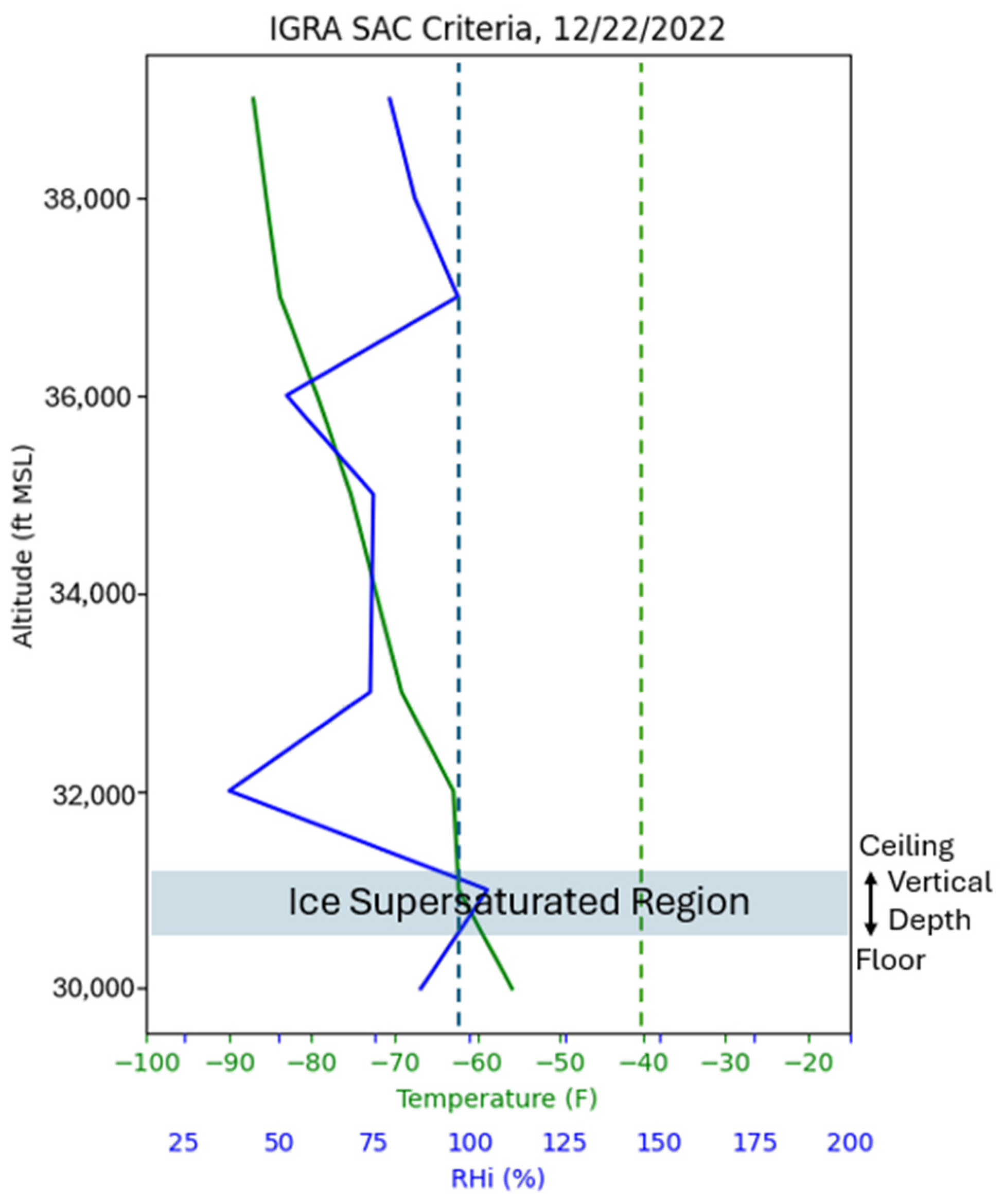
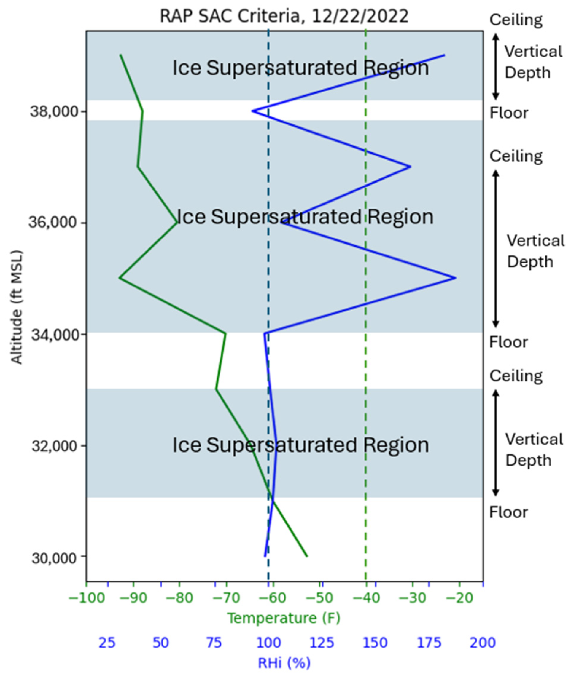
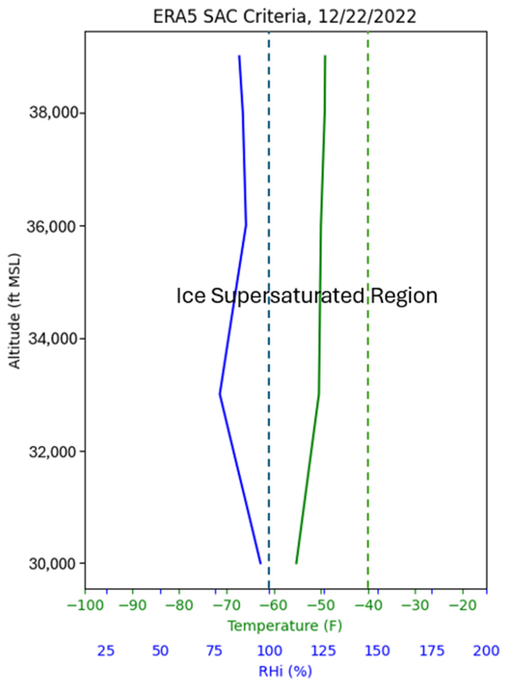
An example of the differences is illustrated for 22 December 2022 (Figure 2, Figure 3 and Figure 4). The green line represents temperature, and the blue line represents RHI. The dashed vertical lines are placed at the ISSR values for each parameter. The IGRA data met the criteria for an ISSR from FL300 to FL310. RAP meets the criteria for ISSRs: one from FL310 to FL330, another from FL350 to FL370, and lastly at FL390 to FL400. ERA5 did not meet the criteria for an ISSR.

Figure 2.
ISSR identification on the same date and at the same location across IGRA for 22 December 2022.

Figure 3.
ISSR identification on the same date and at the same location across RAP for 22 December 2022.
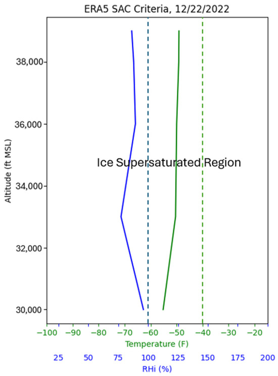
Figure 4.
ISSR identification on the same date and at the same location across ERA5 for 22 December 2022.
For every day on which an ISSR formed over Sterling, Virginia, for at least one hour, a day was counted from 16 December 2022 to 31 July 2024 (593 days) (Table 10).
Table 10.
Daily counts of ISSRs across three databases.
IGRA identified an ISSR on 44.4% of the days, ERA5 identified an ISSR on 77.4% of the days, and RAP on 47.4% of the days. RAP was closest to IGRA, while still overreporting ISSR prevalence by 18 days, as IGRA serves as the ground truth. ERA5 substantially overreported ISSR prevalence, by 196 days.
Under the assumption that IGRA is the ground truth, out of 594 days of observation, there were 4 days on which IGRA identified an ISSR and neither RAP nor ERA5 identified an ISSR. There were fifty-nine (59) days on which IGRA and RAP marked an ISSR. There were thirty-five (35) days on which IGRA and ERA5 marked an ISSR. There were 165 days when all three databases showed an ISSR.
Since flights transit high-altitude airspace at fixed flight levels, an analysis of the identification of ISSRs across the three weather databases was performed at each flight level from 16 December 2022 to 31 July 2024 (593 days) (Table 11). The baseline IGRA data showed the greatest number of days, 116, on which an ISSR occurred at FL 340. The greatest number of days on which an ISSR occurred was 133 days at FL 320 for RAP and 252 days for FL 330 for ERA5. These results indicate significant differences by flight level, which could make selecting the step-climb/descent cruise flight levels for contrail avoidance inaccurate.
Table 11.
Daily counts of ISSRs across RAP, ERA5, and IGRA by flight level.
5. Conclusions
Research simulation models and flight planning decision support tools are being applied to identifying the location of ISSRs for the purpose of contrail inventory and/or contrail avoidance. Twenty-two (22) peer-reviewed papers describing the data, algorithms, and equations used for ISSR identification were reviewed and evaluated.
The review identified three different sources of atmospheric data that were used: the National Oceanic and Atmosphere Administration (NOAA) Rapid Refresh (RAP), the European Centre for Medium-Range Weather Forecasts Reanalysis (ERA5), and the Integrated Global Radiosonde Archive (IGRA). Whereas NOAA and ECMRWF are physics-based atmospheric forecasts, IGRA is a global dataset of radiosonde (weather balloon) observations. IGRA includes atmospheric profiles of temperature, humidity, and wind from stations around the world.
ISSRs are typically under 10 km wide and under 100 m high. Given their narrow structure and given the coarse vertical resolution of atmospheric models, ISSRs are often missed.
Three parameters were used across all of the studies: temperature, pressure, and relative humidity to water (RHW). A critical step in the analyses is the conversion of RHW into relative humidity to ice (RHI). This conversion is conducted using the Goff–Gratch equations [16].
Discrepancies across the values of the parameters in atmospheric forecast databases are present. Using the radiosonde data at a specified geographic location as a baseline, the temperature discrepancies across the flight levels averaged −4.5 °F and 2.4 °F across two different atmospheric databases. For relative humidity to water (RHW), the deviations averaged at 6.6% and 24.8% across the same flight levels when compared to the radiosonde reference data.
Furthermore, over an 18-month period at the same geographic location, the radiosonde data and two atmospheric forecast databases identified ISS conditions on 44%, 47%, and 77% of the days, respectively. An analysis by flight level identified the discrepancies on any given day. The greatest number of days on which an ISSR was recorded was 133 days at FL 320 for RAP and 252 days for FL 330 for ERA5. These results indicate significant differences by flight level, which could make selecting the step-climb/descent cruise flight levels for contrail avoidance inaccurate.
Based on these results, the forecast databases overestimated ISSRs compared to the radiosonde data. These findings underscore the variability inherent in atmospheric datasets and the conversion methods, highlighting potential areas for refinement in ISSR prediction.
5.1. Limitations
A key limitation of this study came from the different altitude reports requiring the interpolation of the temperature and RHI values to analyze the data at 1000-foot increments. For example, ERA5 only reports altitude at four flight levels out of ten in this study. This limitation is further amplified in the necessity of calculating RHI from RHW, as no direct measurement of RHI exists in any of the databases. As ISSRs are large laterally but short vertically, it is crucial to understand the vertical span of ISSRs. This is so that the application of navigational avoidance may be successful in terms of contrail mitigation and a reduction in the impact of aviation on climate.
Additionally, radiosondes drift over time, limiting the spatial consistency of the ground truth data from IGRA. On average, in the Washington DC airspace, IGRA radiosondes drifted 157 nautical miles and drifted up to 3107 nautical miles in a study from 2019 to 2023 [4].
5.2. Future Work
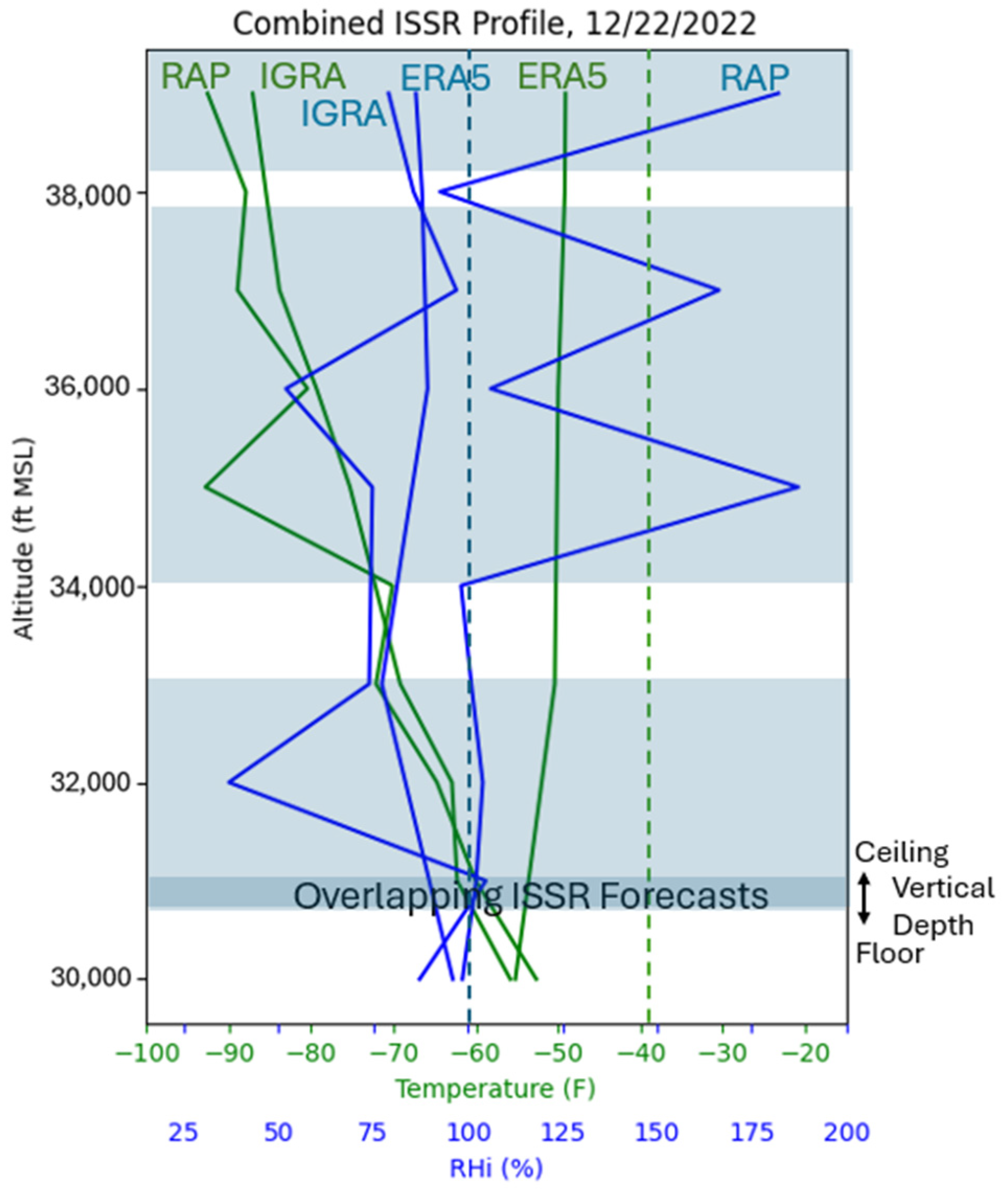
Future work will investigate the generation of an ensemble ISSR forecast for a specific location. The parameters of temperature and relative humidity with respect to ice are gathered from the IGRA, RAP, and ERA5 databases and plotted onto the same chart to determine the overlap between databases in the threshold values, and thus increased confidence, in forecasts. If multiple databases agree that the ISSR criteria are met, then it is more likely that an airplane will form a contrail when flying through this area. An example for a single day and a uniform location and altitude range is illustrated in Figure 5.

Figure 5.
Combined ISSR profile on the same date and at the same location across the IGRA, RAP, and ERA5 for 22 December 2022.
Author Contributions
Conceptualization: A.T.R.-T. and L.S. Methodology: A.T.R.-T., L.S. and K.E. Software: A.T.R.-T. and K.E. Formal analysis:, A.T.R.-T. Resources: A.T.R.-T. and L.S. Writing—original draft preparation: A.T.R.-T. and L.S. Writing—review and editing: A.T.R.-T. and L.S. Visualization: A.T.R.-T. Supervision: L.S. Project administration: L.S. Funding acquisition: L.S. All authors have read and agreed to the published version of the manuscript.
Funding
This research received no external funding.
Institutional Review Board Statement
Not applicable.
Informed Consent Statement
Not applicable.
Data Availability Statement
The original contributions presented in this study are included in the article. Further inquiries can be directed to the corresponding author.
Acknowledgments
The authors acknowledge the technical and editorial comments and suggestions from Donglian Sun, Edward Oughton, Ronald Resmini, Shahab Aref, John Shortle, Brett Berlin (GMU), Judith Rosenow (Technical University Dresden), Andrew Lacher (NASA), Terry Thompson (S&P Global), and Joachim Majholm (Blue Line). No external funding was used to conduct this research.
Conflicts of Interest
The authors declare no conflicts of interest.
Abbreviations
| Abbreviation | Meaning |
| DWD | Deutscher Wetterdienst |
| ECMWF | European Centre for Medium-Range Weather Forecasts |
| EDT | Eastern Daylight Time |
| ERA5 | ECMWF Atmospheric Reanalysis |
| GRIB2 | General Regularly Distributed Information in Binary |
| GSI | Gridpoint Statistical Interpolation |
| GWP20 | Global Warming Potential Time Horizon, 20-Year Equivalent |
| HRES | High-Resolution Forecast |
| HRRR | High-Resolution Rapid Refresh |
| IAGOS | In-Service Aircraft for a Global Observing System |
| ICON | ICOsahedral Nonhydrostatic |
| IFS | Integrated Forecasting System |
| IGRA | Integrated Global Radiosonde Archive |
| ISA | International Standard Atmosphere |
| NCEI | National Centers for Environmental Information |
| NOAA | National Oceanic and Atmospheric Administration |
| RAP | Rapid Refresh |
| RHI | Relative Humidity with respect to Ice |
| RHW | Relative Humidity with respect to Water |
| SAC | Schimdt-Appleman Criteria |
| WRF-ARF | Advanced Research Weather Research and Forecasting Model |
References
- Schumann, U. On Conditions for Contrail Formation from Aircraft Exhausts. Meteorol. Z. 1996, 5, 4–23. [Google Scholar] [CrossRef]
- Schumann, U. A contrail cirrus prediction model. Geosci. Model Dev. 2012, 5, 543–580. [Google Scholar] [CrossRef]
- Gierens, K.; Spichtinger, P. On the size distribution of ice-supersaturated regions in the upper troposphere and lowermost stratosphere. Ann. Geophys. 2000, 18, 499–504. [Google Scholar] [CrossRef]
- Ebright, K.; Sherry, L. Characteristics of Ice Super Saturated Regions in Washington, D.C. Airspace (2019–2023). Aerospace 2024, 11, 587. [Google Scholar] [CrossRef]
- Kärcher, B.; Burkhardt, U.; Bier, A.; Bock, L.; Ford, I.J. The microphysical pathway to contrail formation. J. Geophys. Res. Atmos. 2015, 120, 7893–7927. [Google Scholar] [CrossRef]
- Schumann, U.; Graf, K.; Mannstein, H. Potential to reduce the climate impact of aviation by flight level changes. In Proceedings of the 3rd AIAA Atmospheric Space Environments Conference, Honolulu, HI, USA, 27–30 June 2011. [Google Scholar] [CrossRef]
- Lee, D.S.; Fahey, D.W.; Skowron, A.; Allen, M.R.; Burkhardt, U.; Chen, Q.; Doherty, S.J.; Freeman, S.; Forster, P.M.; Fuglestvedt, J. The contribution of global aviation to anthropogenic climate forcing for 2000 to 2018. Atmos. Environ. 2021, 244, 117834. [Google Scholar] [CrossRef] [PubMed]
- GE Aerospace and NASA Partnering on Flight Tests to Accelerate Industry’s Understanding of Contrails|GE Aerospace News. Available online: https://www.geaerospace.com/news/press-releases/ge-aerospace-and-nasa-partnering-flight-tests-accelerate-industrys-understanding (accessed on 17 November 2024).
- Sherry, L.; Thompson, T. Primer on Aircraft Induced Clouds and Their Global Warming Mitigation Options. Transp. Res. Rec. 2020, 2674, 827–841. [Google Scholar] [CrossRef]
- Avila, D.; Sherry, L.; Thompson, T. Reducing global warming by airline contrail avoidance: A case study of annual benefits for the contiguous United States. Transp. Res. Interdiscip. Perspect. 2019, 2, 100033. [Google Scholar] [CrossRef]
- Roosenbrand, E.; Sun, J.; Hoekstra, J. Optimizing Global Flight Altitudes for Contrail Reduction: Insights from Open Flight and Weather Balloon Data. In Proceedings of the Fifteenth USA/Europe Air Traffic Management Research and Development Seminar (ATM2023), Savannah, GA, USA, 5–10 June 2023. [Google Scholar]
- Sausen, R.; Hofer, S.; Gierens, K.; Bugliaro, L.; Ehrmanntraut, R.; Sitova, I.; Walczak, K.; Burridge-Diesing, A.; Bowman, M.; Miller, N. Can we successfully avoid persistent contrails by small altitude adjustments of flights in the real world? Meteorol. Z. 2023, 33, 83–98. [Google Scholar] [CrossRef]
- Rosenow, J.; Fricke, H.; Luchkova, T.; Schultz, M. Minimizing contrail formation by rerouting around dynamic ice-supersaturated regions. Aeronaut. Aerosp. Open Access J. 2018, 2, 105–111. [Google Scholar] [CrossRef]
- Teoh, R.; Schumann, U.; Majumdar, A.; Stettler ME, J. Mitigating the Climate Forcing of Aircraft Contrails by Small-Scale Diversions and Technology Adoption. Environ. Sci. Technol. 2020, 54, 2941–2950. [Google Scholar] [CrossRef] [PubMed]
- Teoh, R.; Schumann, U.; Stettler, M. Beyond Contrail Avoidance: Efficacy of Flight Altitude Changes to Minimise Contrail Climate Forcing. Aerospace 2020, 7, 121. [Google Scholar] [CrossRef]
- Goff, J.A.; Gratch, S. Low-pressure properties of water from −160 to 212 °F, in Transactions of the American Society of Heating and Ventilating Engineers. In Proceedings of the 52nd annual meeting of the American Society of Heating and Ventilating Engineers, New York, NY, USA, 10–13 June 1946; pp. 95–122. [Google Scholar]
- Teoh, R.; Engberg, Z.; Schumann, U.; Voigt, C.; Shapiro, M.; Rohs, S.; Stettler, M. Global aviation contrail climate effects from 2019 to 2021. Atmos. Chem. Phys. 2024, 24, 6071–6093. [Google Scholar] [CrossRef]
- Schmidt, E. Die Entstehung von Eisnebel aus den Auspuffgasen von Flugmotoren (Other 44); Heft 44; Oldenbourg, V.R., Ed.; Schriften der Deutschen Akademie der Luftfahrtforschung: München, Germany, 1941; Available online: https://elib.dlr.de/107948/ (accessed on 12 August 2024).
- Appleman, H. The Formation of Exhaust Condensation Trails by Jet Aircraft. Bull. Am. Meteorol. Soc. 1953, 34, 14–20. [Google Scholar] [CrossRef]
- Rapid Refresh (RAP). Available online: https://rapidrefresh.noaa.gov/ (accessed on 12 August 2024).
- European Centre for Medium-Range Weather Forecasts. ECMWF Reanalysis 5th Addition (ERA5). Available online: https://www.ecmwf.int/en/forecasts/dataset/ecmwf-reanalysis-v5 (accessed on 12 August 2024).
- Integrated Global Radiosonde Archive (IGRA). National Centers for Environmental Information (NCEI). Available online: https://www.ncei.noaa.gov/products/weather-balloon/integrated-global-radiosonde-archive (accessed on 12 August 2024).
- Weather and Climate—Deutscher Wetterdienst—Homepage. Available online: https://www.dwd.de/DE/Home/home_node.html (accessed on 11 December 2024).
- Avila, D.; Sherry, L. Method for analysis of Ice Super Saturated Regions (ISSR) in the U.S. airspace. In Proceedings of the 2016 Integrated Communications Navigation and Surveillance (ICNS), Herndon, VA, USA, 19–21 April 2016; pp. 10B2-1–10B2-9. [Google Scholar] [CrossRef]
- Borella, A.; Boucher, O.; Shine, K.; Stettler, M.; Tanaka, K.; Teoh, R.; Bellouin, N. The importance of an informed choice of CO2-equivalence metrics for contrail avoidance. EGUsphere, 2024; preprint. [Google Scholar] [CrossRef]
- Contrails Map. Contrails.Org. Available online: https://map.contrails.org/ (accessed on 26 March 2024).
- Dietmüller, S.; Ponater, M.; Sausen, R.; Hoinka, K.-P.; Pechtl, S. Contrails, Natural Clouds, and Diurnal Temperature Range. J. Clim. 2008, 21, 5061–5075. [Google Scholar] [CrossRef]
- Molloy, J.; Teoh, R.; Harty, S.; Koudis, G.; Schumann, U.; Poll, I.; Stettler, M. Design Principles for a Contrail-Minimizing Trial in the North Atlantic. Aerospace 2022, 9, 375. [Google Scholar] [CrossRef]
- Roosenbrand, E.; Sun, J.; Hoekstra, J. Examining Contrail Formation Models with Open Flight and Remote Sensing Data. In Proceedings of the SESAR Innovation Days 2022, Budapest, Hungary, 5–8 December 2022. [Google Scholar]
- Schumann, U.; Heymsfield, A.J. On the Life Cycle of Individual Contrails and Contrail Cirrus. Meteorol. Monogr. 2017, 58, 3.1–3.24. [Google Scholar] [CrossRef]
- Teoh, R.; Engberg, Z.; Shapiro, M.; Dray, L.; Stettler, M. The high-resolution Global Aviation emissions Inventory based on ADS-B (GAIA) for 2019–2021. Atmos. Chem. Phys. 2024, 24, 725–744. [Google Scholar] [CrossRef]
- Frias, A.M.; Shapiro, M.L.; Engberg, Z.; Zopp, R.; Soler, M.; Stettler ME, J. Feasibility of contrail avoidance in a commercial flight planning system: An operational analysis. Environ. Res. Infrastruct. Sustain. 2024, 4, 015013. [Google Scholar] [CrossRef]
- Thompson, G.; Scholzen, C.; O’Donoghue, S.; Haughton, M.; Jones, R.L.; Durant, A.; Farrington, C. On the fidelity of high-resolution numerical weather forecasts of contrail-favorable conditions. Atmos. Res. 2024, 311, 107663. [Google Scholar] [CrossRef]
- US Department of Commerce. Pressure Altitude Calculator. NOAA’s National Weather Service. Available online: https://www.weather.gov/epz/wxcalc_pressurealtitude (accessed on 2 October 2024).

Disclaimer/Publisher’s Note: The statements, opinions and data contained in all publications are solely those of the individual author(s) and contributor(s) and not of MDPI and/or the editor(s). MDPI and/or the editor(s) disclaim responsibility for any injury to people or property resulting from any ideas, methods, instructions or products referred to in the content. |
© 2025 by the authors. Licensee MDPI, Basel, Switzerland. This article is an open access article distributed under the terms and conditions of the Creative Commons Attribution (CC BY) license (https://creativecommons.org/licenses/by/4.0/).