Article

Predicting Lightning from Near-Surface Climate Data in the Northeastern United States: An Alternative to CAPE

by
Charlotte Uden
1,*,
Patrick J. Clemins
2,3 and
Brian Beckage
1,3,4,5,*
1
Department of Plant Biology, University of Vermont, Burlington, VT 05405, USA
2
Vermont EPSCoR, University of Vermont, Burlington, VT 05405, USA
3
Department of Computer Science, University of Vermont, Burlington, VT 05405, USA
4
Gund Institute for Environment, University of Vermont, Burlington, VT 05405, USA
5
Vermont Complex Systems Institute, University of Vermont, Burlington, VT 05405, USA
*
Authors to whom correspondence should be addressed.
Atmosphere 2025, 16(11), 1298; https://doi.org/10.3390/atmos16111298
Submission received: 1 October 2025 / Revised: 29 October 2025 / Accepted: 31 October 2025 / Published: 17 November 2025
(This article belongs to the Section Atmospheric Techniques, Instruments, and Modeling)

Abstract

Lightning is a critical driver of natural wildfire ignition and ecosystem dynamics, but existing prediction models rely on upper-air predictors such as convective available potential energy (CAPE) that are absent from paleoclimate reconstructions. To enable long-term reconstructions of lightning activity, we developed and evaluated statistical models based solely on near-surface climate variables: temperature, precipitation, humidity, surface air pressure, wind, and shortwave radiation. Using ERA5 reanalysis and Vaisala Lightning Detection Network data (2005–2010) for the Northeastern United States, we compared linear regression, gamma generalized linear models, and Bayesian gamma models against CAPE-based benchmarks. While CAPE-based models outperformed models based on individual near-surface predictors, they showed limitations when predicting temporal anomalies. Models incorporating multiple near-surface predictors consistently outperformed CAPE-based models, reproducing observed spatial gradients, interannual variability, and strike rate distributions. Gamma generalized linear models achieved the strongest overall performance, balancing realistic, non-negative predictions with accuracy across error- and correlation-based metrics, while Bayesian models better captured the distribution of strike rates but sacrificed spatial precision. Our results demonstrate that near-surface predictors provide a viable alternative for lightning prediction when upper-air data are unavailable, providing a methodological pathway for reconstructing long-term seasonal lightning variability and its role in climate-fire interactions.

1. Introduction

Lightning has played a fundamental role in shaping wildfire regimes and terrestrial ecosystems for millions of years, serving as both a natural disturbance agent and an ecological driver [1]. In fire-adapted ecosystems, wildfires create mosaic patterns of succession [2,3] and promote biodiversity [4]. The efficiency of lightning in igniting wildfires depends on fuel availability and weather conditions [5,6,7] both of which are sensitive to climate. As global temperatures rise, shifts in atmospheric convection may alter lightning frequency and distribution, potentially driving a rise in lightning-ignited wildfires [8] and triggering ecological transitions in vulnerable regions [5,9].
This interaction between climate and lightning-caused wildfire is increasingly relevant to the Northeastern United States (NE US) given projected increases in fire risk across the region. Regional climate projections predict rises in temperature (defined by milder winters and warmer summers), and longer droughts (flanked by extreme precipitation events) [10,11], which are likely to intensify fire weather conditions in the region [12,13,14,15]. Understanding the joint role of climate and lightning in driving wildfire is therefore critical for anticipating future changes.
One way to inform this future is by examining the past. Reconstructing lightning, wildfire, and vegetation dynamics over the last millennium can provide a baseline for understanding natural variability and for evaluating ecosystem resilience to climate change. However, existing lightning prediction models are ill-suited for this task. Most rely on upper-air predictors including convective available potential energy (CAPE) [8,9,16,17], lifting condensation level, column saturation fraction [16], cloud top height, updraft intensity, cold cloud depth [18,19], convective mass flux [20,21], cloud radius, graupel-pellet concentration, updraft speed [22], and atmospheric electric field [23]. These predictors are available in modern reanalyses and global climate model outputs, but they are not available in paleoclimate reconstructions, which instead provide long-term records of near-surface variables from proxy data [24,25,26].
This limitation creates a methodological gap: lightning models developed for modern datasets cannot be directly applied to paleoclimate reconstructions. To address this gap, we develop lightning prediction models based solely on near-surface climate variables. By doing so, we provide a framework for reconstructing historical lightning activity in the NE US over the last millennium, and for linking these reconstructions to fire and vegetation response. We replace CAPE-based predictors with six near-surface climate variables: temperature, precipitation, humidity, surface air pressure, wind, and shortwave radiation and apply three modeling approaches: a simple linear regression with Gaussian errors, a generalized linear model (GLM) with gamma-distributed errors, and a Bayesian gamma approach. Using ERA5 reanalysis data [27] and Vaisala Lightning Database records [28] (2005–2010) for the NE US, we benchmark these approaches against modern observations, providing a foundation for paleoclimate applications where only near-surface variables are available.

2. Materials and Methods

2.1. Data

This study develops alternative lightning prediction models that replace an upper-air predictor with near-surface predictors available in paleoclimate reconstructions. We selected the 2005–2010-year period because we are limited by the Vaisala Lightning Detection Network’s [28] data distribution policies. These specific years provide the maximum overlap between available lightning observations and available paleoclimate reconstructions, ensuring continuity between model development and downstream applications in lightning, wildfire, and vegetation dynamics in the NE US.
CAPE (J/kg) and the product of CAPE and Precipitation (CAPE × precip) were chosen as upper-air predictors to compare with near-surface predictors, due to their effectiveness in predicting lightning in previous work [8,9]. Near-surface predictors include 2 m temperature (°C), instantaneous 10 m wind gust (m/s), mean surface downward shortwave radiation flux (W/m2), surface pressure (Pa), mean total precipitation rate (kg/m2/s), and relative humidity (%), calculated from temperature and 2 m dew point temperature). These six climate variables were selected because they are included in the paleoclimate reconstructions available for the NE US [29]. ERA5 reanalysis data were obtained from the Copernicus Climate Change Service [27] and are on a 0.25° × 0.25° resolution grid (corresponding, in the study region, to an approximately 28 km by 20 km grid) that covers New England and New York. The data span a six year period (2005–2010) on an hourly time step. Relative humidity (following the Magnus–Tetens approximation, [30]) and the CAPE × precip term were calculated at the hourly scale before being summarized to monthly averages.
The Vaisala National Lightning Detection Network [28] provided daily lightning counts for the 2005–2010 period. The data were collected by ground-based stations that detect electromagnetic activity emitted during a lightning strike. Vaisala achieved cloud-to-ground (CG) detection efficiencies of ~90–95% across the continental US during 2005–2010 [31,32]. Intra-cloud (IC) strikes were more challenging to detect during this period, with efficiencies below 20%, though classification algorithms improved over time [33,34]. NLDN distinguishes CG from IC strikes based on electromagnetic waveform characteristics, with CG strikes producing distinct ground-return signatures. Only CG lightning strikes were used in this analysis (not IC or total strikes). The dataset includes the date, time, location, and number of strokes for each CG lightning strike. A CG strike consists of all the CG strokes that occur within 10 km and 1 s of each other. Here, we are interested in modeling CG strikes, not strokes. To address the challenges of zero-inflated data, we followed the methods of Moon and Kim (2020) [17], excluding the winter months (October to April), which reduced the percentage of zeros in the daily lightning count data from 93% to 85%. This exclusion has little effect on the analysis, as lightning activity during these months is minimal compared to the summer season (Figure 1a). Furthermore, our focus was on the fire season months when lightning plays an ecological role.
To match the lightning point data to the ERA5 grid, lightning point locations were assigned to a raster layer with the same spatial resolution as the ERA5 grid. Lightning strikes that occurred within a given cell during a given summer month (May to September) were summed and divided by the grid cell area to calculate a strike rate, expressed in strikes per km2 per month, matching the units in Romps et al. (2014) [8]. This procedure was carried out for each summer season across the entire study period (2005–2010) and region (New England and New York). Aggregating the data this way allowed for a consistent spatial and temporal alignment of the lightning data with the ERA5 climate data and kept the target variable (lightning strike rate) above zero, facilitating downstream modeling. The data include 3246 total observations of summer mean values, corresponding to 541 grid cells across the NE US over six years. These observations were randomly split across all years into train (80%) and test (20%) sets.

2.2. Model Definitions

Since upper-air variables such as CAPE are not typically included in long-term historical climate reconstructions, they cannot be used to model lightning strike rates over these periods. To address this limitation, we build upon existing, well performing models (Baseline models, C1–C5) from Chen et al. (2021) [9] that predict lightning strikes from CAPE × precipitation [9]. We test three modeling approaches: (1) a linear model with Gaussian errors (Normal LMs, N1–N13), (2) a GLM with gamma-distributed errors (gamma GLMs, G1–G13), and (3) a Bayesian approach that models the full predictive distribution (Bayesian gamma models, B1–B13). Within each approach, we applied both upper-air and near-surface climate predictors, as well as the additive effects of multiple near-surface predictors. Variable selection for the additive models was guided by a combination of random forest importance (mean decrease in impurity and increase in mean square error) and exploratory visual analysis; variables were added stepwise beginning with shortwave radiation (the most important predictor), allowing us to assess the contribution of each variable to predictive skill. Interaction terms between near-surface predictors were also evaluated to account for potential nonlinear processes in lightning formation, but this consistently degraded performance, so final models retained only additive structures.
Predictor variables were standardized using z-score transformation prior to fitting the Normal LMs, Gamma GLMs, and Bayesian Gamma models. The baseline CAPE × precipitation models, which rely on a single predictor, were fitted without standardization to maintain comparability with Chen et al. (2021) [9]. Because these baseline models include only one predictor, standardization is not required to balance the influence of multiple variables, and using raw values preserves consistency with the original methods in Chen et al. (2021) [9]. We emphasize interpretable statistical approaches rather than black-box machine learning models, as the limited sample size (3246 observations) increases the risk of overfitting in high-capacity algorithms.

2.2.1. Baseline Models (C1–C5)

The initial model set (C1–C5 in Table 1 and Table 2) is based on five models from Chen et al. (2021) [9] and serves as a benchmark for comparing established approaches in the literature with the models developed in this study. All five models predict lightning strike rate ( r s   ) from CAPE × precip (CAPE × Pr). These models employ different functional forms but share an assumption of normally distributed residuals and constant variance. They include:
  • C1 (Power Law Model): r s   = a(CAPE × Pr)b, where a and b are estimated via log-log regression.
  • C2 (Power Law, Linear Optimization): Follows the same functional form as C1 but applies nonlinear least squares optimization directly without log transformation.
3.
C3 (Scaling Model): r s   = a(CAPE × Pr), assumes direct proportionality between r s   and CAPE × Pr.
4.
C4 (Non-Parametric Model): Uses a lookup table of mean strike rates across binned values of CAPE × Pr.
5.
C5 (Ensemble Model): Applies the ensemble mean of C1–C4.
These models have been retrained on data for the study region (NE US). Fitting was conducted in R [35] using the built in linear model function for models C1 and C3, and a nonlinear least squares function for model C2. These models assume normally distributed residuals and constant variance.

2.2.2. Linear Models (N1–N13)

These models (N1–N13, Table 1 and Table 3) modify the baseline approach by incorporating near-surface climate variables as predictors. Lightning strike rate is modeled as a function of climate using a Gaussian error distribution:
E [ r s i ] = a + b · c l i m a t e i + ε i ~ N ( 0 , σ 2 )
where E r s i is the observed lightning strike rate for the i t h observation, a is the intercept, b is the regression coefficient for the climate predictor(s), and ε i is the normally distributed error term with variance σ 2 . These models assume equal variance across climate conditions and that residuals are normally distributed.
Models N1 and N2 apply CAPE and CAPE × precip, models N3–N8 apply single near-surface climate predictors (relative humidity, shortwave radiation, temperature, surface pressure, precipitation, and wind), and models N9–N13 progressively increase model complexity by exploring the combined effects of near-surface climate predictors, with N13 modeling lightning strike rate as a function of all six near-surface climate variables. Models were fitted using standard linear modeling techniques in R [35]. Note that the Normal linear models do not constrain predictions to non-negative values, so occasional negative strike rates were produced. To evaluate their impact, we compared model performance (see below) with and without truncating negatives to zero. The skill score, correlation, and nRMSE differed only marginally (changes < 0.01), confirming that negative values were rare and had negligible influence on model evaluation. Negative values were therefore retained, rather than truncated.

2.2.3. Gamma GLMs (G1–G13)

To better account for the right-skewed nature of lightning strike rates and ensure non-negative predictions, the gamma GLMs (G1–G13 in Table 1 and Table 4) replace the Normal error distribution with a gamma error distribution and employ a log-link function:
E r s i = e x p ( a + b · c l i m a t e i )
with
r s i   ~   G a m m a μ i   ,   ϕ ,     V a r ( r s i ) = ϕ μ i 2
where r s i   is the observed lightning strike rate for the i th observation, E r s i is the expected mean strike rate, a is the intercept, b is the coefficient for the climate predictor(s), and ϕ is the dispersion parameter. In this formulation, the stochastic error is explicitly represented by the Gamma-distributed residuals around the mean, in contrast to the Gaussian residuals of the linear models.
These models maintain consistency with the Linear Models by applying the same numerical naming convention: models G1–G2 provide a reference with upper-air predictors (CAPE and CAPE × precip), while G3–G13 explore individual and combined effects of near-surface predictors on lightning strike rates (again, with G13 including all six near-surface variables). These models were fitted in R [35] using a GLM function with gamma-distributed errors.

2.2.4. Gamma Bayesian Models (B1–B13)

The final model set (B1–B13 in Table 1 and Table 5) builds upon the gamma GLMs by incorporating parameter uncertainty within a Bayesian framework. Instead of predicting point estimates for the expected mean lightning strike rates, these models estimate the full predictive distribution by sampling lightning strike rate from the gamma distribution:
r s i   ~   G a m m a α i , β i
where the shape ( α i ) and scale ( β i ) parameters are linear functions of climate predictor(s) at the i th observation:
α i = a α + b α · c l i m a t e i
β i = a β + b β · c l i m a t e i
where { a α , a β } are intercepts and { b α , b β } are coefficients for α and β . Priors for the intercepts and coefficients are:
a α ,   a β , b α , b β   ~   N ( 0,1 )
These models repeat the numerical naming convention of the Linear Models and gamma GLMs: B1–B2 model CAPE-based relationships, B3-B8 model individual near-surface climate relationships, and B9–B13 model the additive relationships among near surface climate variables. To ensure that α and β remain positive, models B12 and B13 apply a log link function. Parameter values were estimated in the ‘Rstan’ package [36] using Hamiltonian Monte Carlo with the No-U-Turn Sampler in R [35]. Four Markov Chain Monte Carlo chains were run to estimate the model parameters. Chain convergence was assessed using the Gelman-Rubin statistic and trace plots were examined to confirm parameter stability.

2.3. Model Evaluation

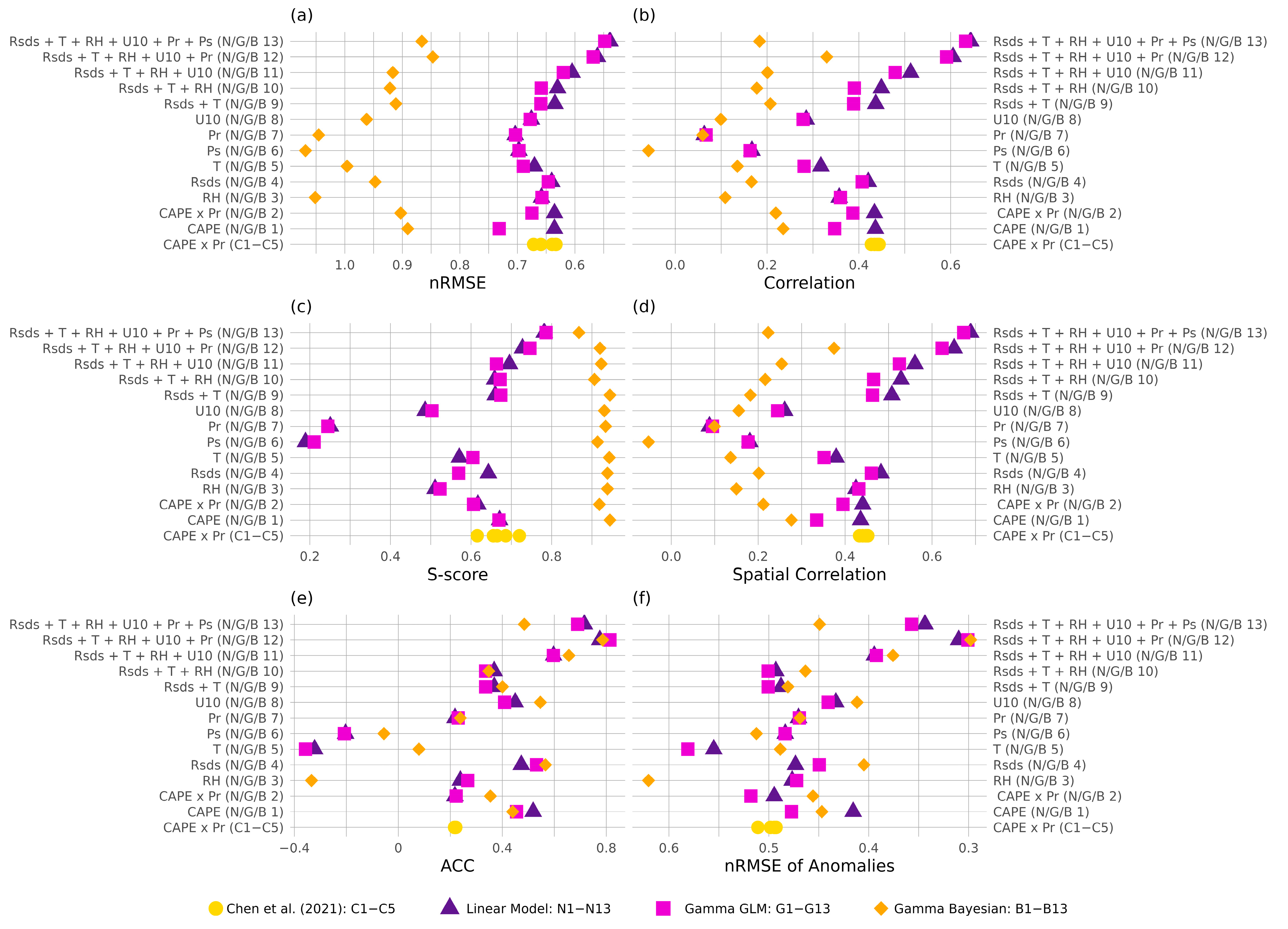
Metrics for comparing model performance (Figure 2) include Normalized Root Mean Squared Error (nRMSE), Pearson correlation between observed and predicted, skill score (S-score), spatial correlation, anomaly correlation coefficient (ACC), and Normalized RMSE of anomalies. All metrics were calculated from the test data.
nRMSE was calculated as RMSE divided by the observed mean. When nRMSE values are greater than 0.6, it is generally interpreted as a good model fit while values below 0.75 indicate high error. Values of correlation between observed and predicted close to 1 suggest good model fit, less than 0.5 suggest weak fit, and less than 0 suggest an inverse relationship.
To assess how well models reproduce the entire probability distribution of values, the S-score (Figure 2c), derived from Perkins et al. (2007) [37], was applied as a metric to compare simulated and observed probability density functions. It was calculated as:
S s c o r e   =   i = 1 n m i n ( P o b s , i ,   P p r e d , i )
where P o b s , i   and P p r e d , i are the relative frequencies of observed and predicted values in bin i, and n is the total number of bins (here, n = 15). S-score values range from 0 to 1, where 1 indicates a perfect match between the model’s simulated distribution and the observed lightning strike rates, and lower values indicate increasing model bias.
Spatial correlation quantifies the ability of models to reproduce the geographic pattern of observed lightning rates. It was calculated as the Pearson correlation coefficient between observed and predicted mean lightning strike rates across all grid cells, averaged over the study period. Values close to 1 indicate that the model successfully reproduces spatial gradients, whereas values near 0 indicate little correspondence with observed spatial patterns.
The anomaly correlation coefficient measures how well models capture interannual variability in lightning occurrence. It is calculated as the Pearson correlation between observed and predicted annual-mean lightning anomalies, obtained by subtracting the six-year mean from each year’s mean. High positive values (approaching +1) indicate that the model reproduces year-to-year fluctuations above and below the mean; values near 0 indicate no skill, and negative values indicate the model predicts anomalies in the opposite direction of observations.
Normalized RMSE of anomalies assesses the magnitude of error in interannual variability. Observed and predicted annual anomalies were first computed relative to the six-year mean, and RMSE was calculated as the square root of the mean squared difference between them. This was then divided by the standard deviation of observed anomalies to get nRMSE of anomalies. Values below 1 indicate that the model reproduces not only the direction but also the magnitude of interannual variability, while values greater than 1 indicate that model error is larger than the observed anomaly record. We acknowledge the use of OpenAI’s ChatGPT (version 4) to aid in code development, and model analysis. All code was tested by the authors.

3. Results

Models C1–C5, based on CAPE × precipitation as in Chen et al. (2021) [9], provided a baseline for comparison. Across all five model variants, nRMSE ranged narrowly from 0.63–0.67, indicating moderate error. Correlations with observed lightning were modest (r ≈ 0.43–0.44), and S-scores were generally high (0.62–0.72) (Figure 2a–c). Relative to other single near-surface predictors, spatial correlations were strong (≈0.44–0.45) (Figure 2d). Anomaly correlations (≈0.22) and nRMSE of anomalies (≈0.49–0.51) from CAPE outperformed single-variable near-surface predictions, except for shortwave radiation (ACC ≈ 0.47–0.57 and nRMSE of anomalies ≈ 0.40–0.47) (Figure 2d–f). While all five models yield similar performance, C1 (Power Law model: a(CAPE × P)b) stands out with the highest S-score.
To assess relative contributions of near-surface predictors, we conducted a random forest importance analysis, which indicated that shortwave radiation, near-surface air temperature, and surface pressure were most influential (Figure 3). However, excluding individual variables generally reduced model performance, so all six predictors were retained in the final multivariable fits.
Under all modeling approaches, models that predict lightning strike rate from a single near-surface climate variable do not perform as well as those that rely on CAPE-based relationships (Figure 2). When applied individually, the near-surface predictors varied widely in their ability to reproduce lightning occurrence. Shortwave radiation performed best, achieving relatively strong spatial correlations (N4: r = 0.48; G4: r = 0.46; B4: r = 0.20) and moderate anomaly correlations (ACC ≈ 0.47–0.57). Wind also showed moderate skill (spatial correlation up to r = 0.41; ACC up to 0.55). By contrast, surface pressure and precipitation performed poorly across nearly all metrics, with correlations near zero and weak or negative ACC values. Temperature and relative humidity fell in between, with modest distributional skill (S-scores ≈ 0.51–0.61) but limited temporal tracking.
Combining predictors markedly improved model skill. For the linear models, performance improved steadily as additional variables were added: from N9 (SWR + T; cor = 0.44, spatial cor = 0.51) through N12 (SWR + T + RH + W + P; cor = 0.61, spatial cor = 0.65), culminating in N13, which used all six predictors and achieved the highest overall scores (nRMSE = 0.54, cor = 0.64, S-score = 0.78, spatial cor = 0.69, ACC = 0.72, nRMSE of anomalies = 0.34). The gamma GLMs followed a similar trajectory, with G13 (all predictors) achieving strong skill (nRMSE = 0.54, cor = 0.63, spatial correlation = 0.67, S-score = 0.79, ACC = 0.69, nRMSE of anomalies = 0.36). However, excluding surface pressure in the Bayesian approach (B12) achieves the best fit across all metrics (nRMSE = 0.86, cor = 00.18, spatial cor = 0.22, S-score = 0.86, ACC = 0.48, nRMSE of anomalies = 0.45).
When evaluating modeling approaches, clear differences emerged. Linear Gaussian models and Gamma GLMs both demonstrated strong improvements when multiple near-surface predictors were included. These models were the only ones to achieve low nRMSE (0.54), high correlation between observed and predicted, and high spatial correlations (>0.65), indicating their ability to reproduce geographic gradients. Bayesian gamma models (B1–B13) stand apart. While ACC and nRMSE of anomalies are comparable to those of the linear models and gamma GLMs and their S-scores were uniformly the highest, they consistently failed to reduce error and capture spatial structure. For example, nRMSE values for models B1–B13 ranged from 0.84–1.07, with no overlap with any other model (nRMSE ≈ 0.54–0.70). nRMSE values less than 0.75 indicate high error, underlining significant performance issues in the Bayesian models.
This divergence between distributional skill and spatiotemporal skill suggests that Bayesian models may be overfit to the central tendency of the data, reproducing overall distributions but not spatial gradients. This is reflected in Figure 4, which compares predictions from models N13, G13, and B12. These models were selected for comparison because they were the best predictors of lightning within their respective modeling approaches. Model B12, which applies the Bayesian approach, more closely reproduces the right skewed distribution of observed lightning strike rates (Figure 4a). However, models N13 and G13 make predictions closer to the observed values, as evidenced by low residuals (Figure 4b).
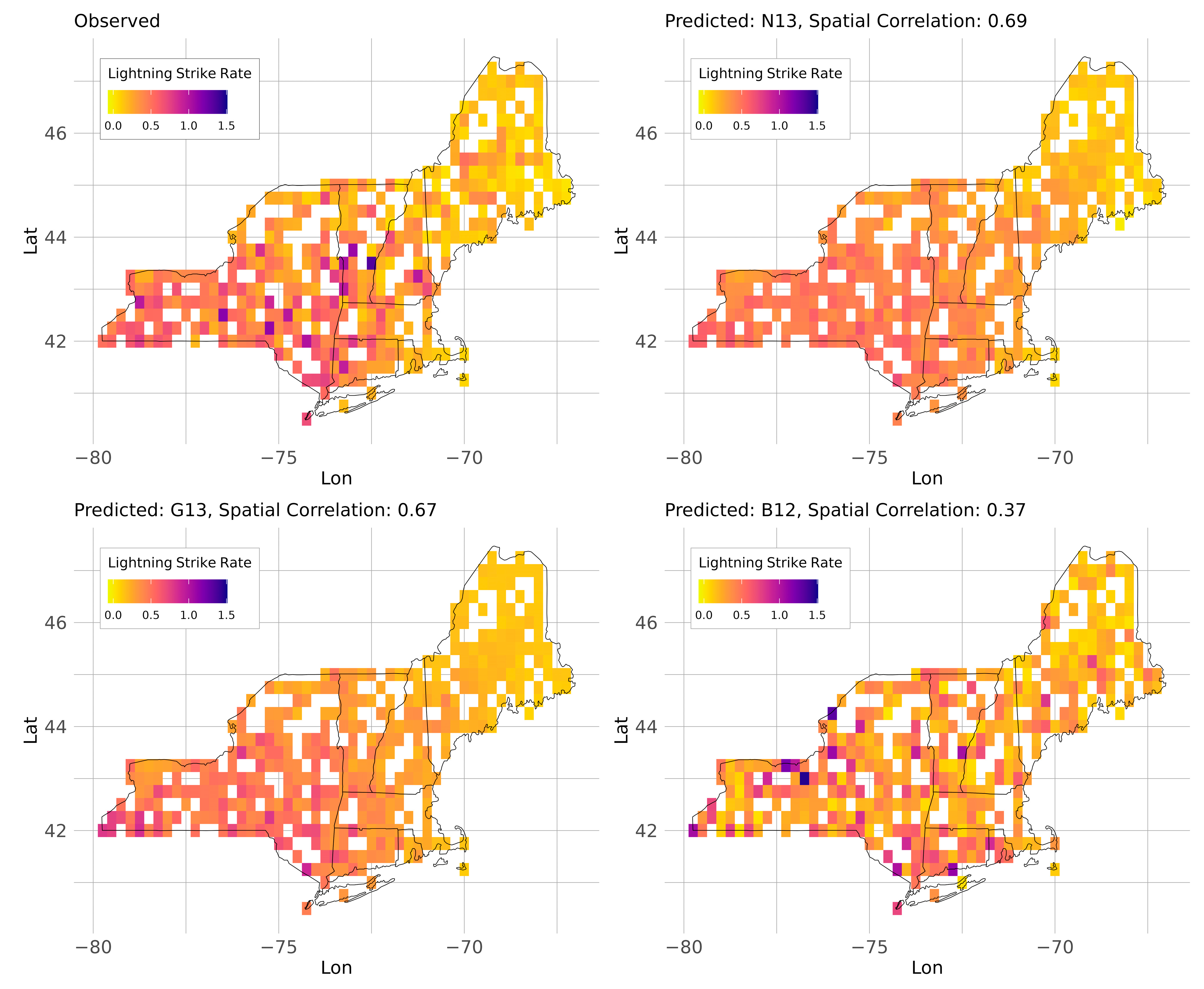
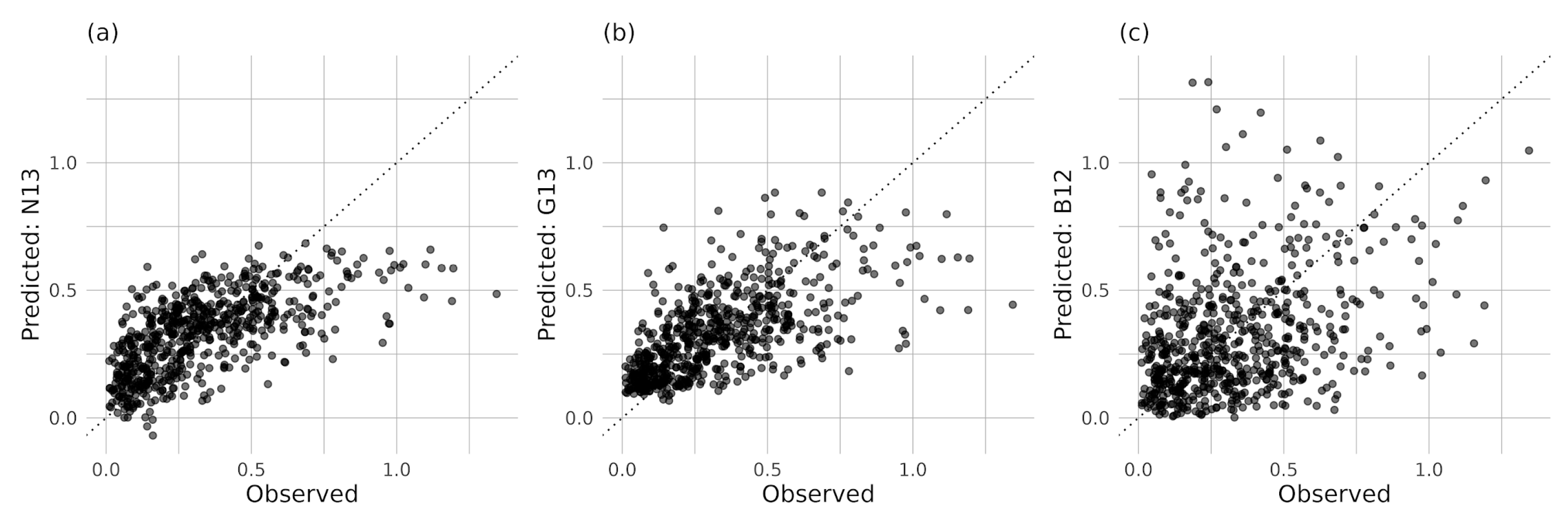
A spatial comparison between observed and predicted lightning strike rates (Figure 5) reflects the spatial correlation values (Figure 2d). Predictions from the linear model (N13) and gamma GLMs (G13) capture the latitudinal gradient seen in the observed data. However, Bayesian model predictions (B12) do not reflect this spatial gradient and the spatial correlation of predictions from the Bayesian approach (B1–B13) never outperform the CAPE-based models (C1–C5). Plotting observed against predicted strike rate (Figure 5) provides additional insight into the accuracy of predictions at each grid point. The 1:1 lines show perfect agreement between predictions and observations. The linear model (Figure 6a) predicts low strike rates well but underestimates higher values. The gamma GLM (Figure 6b) slightly improves upper-end predictions but tends to overestimate low values and still underpredicts beyond ~0.8 strikes/km2/month. The gamma Bayesian model (Figure 6c) captures the observed spread but shows a large amount of scatter around the 1:1 line, indicating much less precision at individual locations.
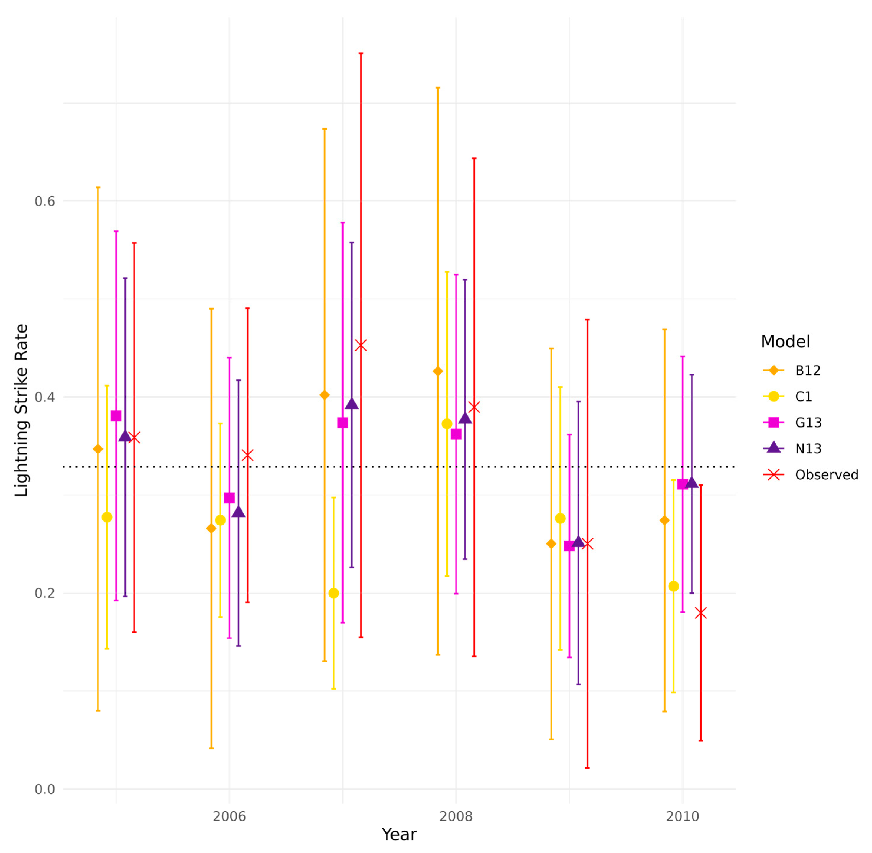
All three modeling approaches that incorporate multiple near-surface predictors (N13, G13, B12) better capture temporal anomalies than the CAPE-based models (Figure 2e,f), both in terms of year-to-year fluctuations (ACC > 0) and magnitude of interannual error (nRMSE of anomalies < 1.0; model error is less than anomaly spread). However, model performance in terms of temporal tracking deteriorates when surface pressure is added to the parameterization (N13, G13, B13), as reflected in lower ACC (from 0.78/0.81/0.79 to 0.72/0.69/0.48 with Ps added, respectively) and higher nRMSE of anomalies (from 0.31/0.30/0.30 to 0.34/0.36/0.45 with Ps added, respectively). Figure 7 compares deviations from the six-year observed average with the outputs of models C1, N13, G13, and B12 (again selected as the best performers within their respective approaches). During the first half the study period, the CAPE-based model (C1) fails to reproduce deviations seen in the observed data, underpredicting lightning strike rate. All four models also underpredict strike rate in 2006 and fail to capture the magnitude of deviation from the mean in 2010. Overall, all models generally track interannual changes in the observed mean.

4. Discussion

Our analysis demonstrates that near-surface predictors, when used in multi-variable models, can outperform CAPE-based approaches. While CAPE-based models capture some aspects of lightning occurrence, they fall short in reproducing spatial gradients, temporal variability, and the magnitude of strike rates. Among modeling approaches, the Gamma GLMs offer the strongest balance across evaluation metrics while ensuring physically realistic (non-negative) predictions. Nonetheless, linear models do achieve slightly higher accuracy despite generating occasional negative values. Incorporating all six near-surface predictors yields the most robust results overall, except when capturing temporal anomalies is the priority. In those cases, excluding surface pressure (models N12/G12) improves ACC and nRMSE of anomalies (Figure 2e,f), though retaining it (models N13/G13) remains advantageous for reproducing spatial gradients (Figure 2d). Bayesian approaches show strength in reproducing overall frequency and temporal distributions but struggle to resolve geographic structure, underscoring the tradeoff between capturing broad statistical patterns and representing spatial dynamics.
This divergence in performance metrics between the simpler models (linear and Gamma GLMs) and Bayesian models reflects fundamental differences in how each approach makes predictions (Table 1). Linear and gamma GLMs estimate mean lightning strike rate ( E r s i ) and optimize for low residual variance, leading to strong point-prediction accuracy. In contrast, Gamma Bayesian models estimate the full distribution of lightning strike rates by modeling both the shape and scale parameters and sampling from the gamma distribution ( r s   ~ G a m m a ( α , β ) ). This enables the model to reproduce variability and extremes (S-score is improved), but at the cost of spatial and point-accuracy (nRMSE and correlations worsen). These findings underscore a broader caution in model selection: validation success on a limited set of metrics may miss weaknesses elsewhere. By testing our models across multiple metrics, we show that, while less sophisticated, simpler models can outperform a more advanced approach such as a Bayesian model.
Capturing lightning extremes is particularly important in the context of wildfire. The S-score applied here was developed by Perkins et al. (2007) as a method for comparing the probability density functions (PDFs) of predictions from climate models with observations [37]. They argue that simply evaluating the mean does not capture the full range of variability within the data and that rare events provide equally important information. This perspective is supported by Katz and Brown (1992), who demonstrate that the tails of a climate distribution are more sensitive to changes in variability than the mean, underscoring the need to model both the mean and distribution of climate events [38].
In this study, however, no single model successfully captured both the observed extremes and accurate point predictions. One contributing factor to this outcome is our decision to train models at seasonal scales, which introduces important trade-offs. Aggregating to a seasonal resolution smooths out storm-level detail. As a result, our models cannot resolve the storm-level processes that produce extreme lightning events and predictions should be interpreted as seasonal tendencies, rather than event-level forecasts.
Despite these limitations, there are advantages to aggregating to a seasonal time scale in the context of our objectives. First, it allows models to learn broader relationships between climate and lightning. Second, long term reanalysis data (including paleoclimate reconstructions) increase in bias and uncertainty at finer timescales. These data do not contain information at the storm level, making lightning predictions from fine-grained data infeasible. Finally, because our primary aim is to understand the long-term response of lightning to climate trends, seasonal aggregation is an appropriate granularity.
Future work can improve the representation of extremes while preserving point accuracy, by (1) developing models at finer temporal scales, which would reduce the influence of single extreme events on seasonal statistics [39,40], and (2) exploring alternative machine-learning methods, which may capture nonlinear relationships between near-surface predictors and lightning occurrence more effectively [41].
Spatial gradients also provide a critical test of model behavior. Models N13 and G13 successfully capture the observed decline in lightning activity with latitude (Figure 5). This gradient has been linked to several factors, including a reduction in cold cloud depth [18,19] and decreasing CAPE at higher latitudes [8], and weaker surface heating due to lower solar insolation [42]. Our results are consistent with this mechanism: both CAPE and shortwave radiation decline with latitude (Figure 1c,g) and shortwave radiation emerged as the strongest near-surface predictor in both the random forest analysis and single-variable models (Figure 2 and Figure 3). Because surface heating and radiation drive convection, the performance of shortwave radiation in predicting lightning frequency highlights its physical relevance, even though it is indirect compared to CAPE.
Beyond shortwave radiation, other near-surface predictors also offer physically meaningful insights, as shown by increased accuracy upon adding them to our models:
1.
Surface pressure saw high importance in the random forest analysis, but low stand-alone performance and degraded temporal accuracy when used in combination with the other five near-surface variables. This is reflected by [43], who found that pressure-derived indices can successfully identify convective environments, but cannot capture the timing of individual events. Pressure does not show large year-to-year variability, particularly at a seasonal resolution, reducing its ability to track interannual changes in lightning.
2.
Surface temperature demonstrated moderate predictive skill relative to other single variable models. Prior studies have shown that elevated surface temperatures coincide with lightning [44], which may reflect boundary-layer thermodynamics, where warmer surface temperatures increase air buoyancy.
3.
Wind speed demonstrated moderate to low importance in the random forest analysis, but performed well in terms of temporal accuracy. Wind near the surface plays a dual role in convective processes. It can aid in the development of a convective storm by delivering warm, humid air and enhancing heat exchange. However, strong surface wind speeds will prevent the temperature and humidity layers associated with convection from forming [45].
4.
Precipitation, by contrast, ranked low in both importance and predictive skill when used alone. While precipitation is often used as a proxy for convective activity, its poor performance here may come from two factors. First, aggregating to a seasonal scale smooths out storm-level events. Second, the ERA5 precipitation data we used includes both convective and stratiform components [27]. Including stratiform precipitation, which is not usually associated with lightning, likely dilutes the signal.
5.
Finally, relative humidity also had low stand-alone importance and temporal accuracy but improved model performance when included with other variables. While relative humidity has been linked to lightning occurrence through its role in cloud formation and convective efficiency [46], it alone does not trigger convection; high relative humidity reduces the energy required for saturation, but without accompanying factors such as instability and lift, storms are unlikely to form. Moreover, surface relative humidity may not represent layers of low or high moisture in the upper atmosphere important to convection.
These findings highlight that the relationship between near-surface variables and lightning are complex and shaped by interactions among multiple atmospheric processes. The relationships identified here for the NE US may not be directly transferrable to other regions and retraining of models will be necessary to account for differing convective regimes. While our models demonstrate that near-surface predictors can match the performance of CAPE, several limitations should be considered. With limited access to lightning observations from Vaisala, the training period is relatively short (2005–2010). Additionally, the NE US is a relatively low-lightning region, limiting our models’ generalizability to regions of high lightning activity. To address this, future work could expand our approach to a longer climatological period and a larger region as the methodological framework we have developed remains widely applicable. By providing a path toward reconstructing lightning activity from long-term paleoclimate datasets, this work helps lay the foundation for improved understanding of past climate-lightning-fire interactions and their relevance for anticipating future wildfire regimes.

5. Conclusions

This study demonstrates that lightning can be predicted from near-surface climate variables alone, providing an alternative to CAPE-based approaches in contexts where upper-air data are unavailable. Gamma GLMs balance realistic, non-negative predictions with strong accuracy. Incorporating all six predictors produced the most robust results, although excluding surface pressure improved temporal anomaly predictions. This framework is transferable to regions outside the NE US, though retraining with local lightning and climate observations is necessary. These advances will enable more robust reconstructions of past seasonal lightning activity and its role in shaping natural wildfire regimes under changing climates.

Author Contributions

Conceptualization, C.U. and B.B.; methodology, C.U., B.B. and P.J.C.; software, C.U. and P.J.C.; validation, C.U.; formal analysis, C.U.; investigation, C.U.; resources, B.B. and P.J.C.; data curation, C.U.; writing—original draft preparation, C.U.; writing—review and editing, C.U., B.B. and P.J.C.; visualization, C.U.; supervision, B.B. and P.J.C.; project administration, C.U., B.B. and P.J.C.; funding acquisition, B.B. All authors have read and agreed to the published version of the manuscript.

Funding

This research received no external funding.

Institutional Review Board Statement

Not applicable.

Informed Consent Statement

Not applicable.

Data Availability Statement

The code used to develop and test the lightning prediction models, and generate tables and figures is available on GitHub under the version tag v2.0 (https://github.com/charliuden/Lightning-Models-Uden-2025/releases/tag/v2.0, (accessed on 28 September 2025)). The processed data used to drive the models, as well as model predictions, parameter estimates, and performance outcomes are archived in Zenodo (https://doi.org/10.5281/zenodo.17220315). Details on data processing and model descriptions can be found in the Methods section. Unprocessed ERA5 climate data are made available from the Copernicus Climate Change Service. Due to the Vaisala National Lightning Detection Network’s data policy, we cannot provide direct access to the raw lightning data, but the data can be requested from Vaisala.

Acknowledgments

We thank the Copernicus Climate Change Service for making ERA5 data freely available and the Vaisala National Lightning Detection Network for providing lightning data. During the preparation of this manuscript, the authors used OpenAI’s DALL·E 3 model via ChatGPT (GPT-4o, September 2025) for the purposes of generating an image of a storm cloud for the graphical abstract. The authors have reviewed and edited the output and take full responsibility for the content of this publication.

Conflicts of Interest

The authors declare no conflict of interest.

Abbreviations

The following abbreviations are used in this manuscript:
NE USNortheastern United States
CAPEConvective Available Potential Energy
PrPrecipitation
RHRelative humidity
RsdsShortwave radiation
TTemperature
PsSurface Pressure
U10Wind speed
CGCloud-to-ground
ICIntra-cloud
GLMGeneralized linear model
nRMSENormalized Root Mean Squared Error
ACCAnomaly correlation coefficient

References

  1. Pausas, J.G.; Keeley, J.E. A Burning Story: The Role of Fire in the History of Life. BioScience 2009, 59, 593–601. [Google Scholar] [CrossRef]
  2. Allen, H.D. Fire: Plant functional types and patch mosaic burning in fire-prone ecosystems. Prog. Phys. Geogr. 2008, 32, 421–437. [Google Scholar] [CrossRef]
  3. Weir, J.M.H.; Johnson, E.A.; Miyanishi, K. Fire Frequency and the Spatial Age Mosaic of the Mixed-Wood Boreal Forest in Western Canada. Ecol. Appl. 2000, 10, 1162–1177. [Google Scholar] [CrossRef]
  4. He, T.; Lamont, B.B.; Pausas, J.G. Fire as a key driver of Earth’s biodiversity. Biol. Rev. 2019, 94, 1983–2010. [Google Scholar] [CrossRef]
  5. Hessilt, T.D.; Abatzoglou, J.T.; Chen, Y.; Randerson, J.T.; Scholten, R.C.; van der Werf, G.; Veraverbeke, S. Future increases in lightning ignition efficiency and wildfire occurrence expected from drier fuels in boreal forest ecosystems of western North America. Environ. Res. Lett. 2022, 17, 054008. [Google Scholar] [CrossRef]
  6. Peterson, D.; Wang, J.; Ichoku, C.; Remer, L.A. Effects of lightning and other meteorological factors on fire activity in the North American boreal forest: Implications for fire weather forecasting. Atmospheric Chem. Phys. 2010, 10, 6873–6888. [Google Scholar] [CrossRef]
  7. Song, Y.; Xu, C.; Li, X.; Oppong, F. Lightning-Induced Wildfires: An Overview. Fire 2024, 7, 79. [Google Scholar] [CrossRef]
  8. Romps, D.M.; Seeley, J.T.; Vollaro, D.; Molinari, J. Projected increase in lightning strikes in the United States due to global warming. Science 2014, 346, 851–854. [Google Scholar] [CrossRef] [PubMed]
  9. Chen, Y.; Romps, D.M.; Seeley, J.T.; Veraverbeke, S.; Riley, W.J.; Mekonnen, Z.A.; Randerson, J.T. Future increases in Arctic lightning and fire risk for permafrost carbon. Nat. Clim. Change 2021, 11, 404–410. [Google Scholar] [CrossRef]
  10. Hayhoe, K.; Wake, C.; Anderson, B.; Liang, X.-Z.; Maurer, E.; Zhu, J.; Bradbury, J.; DeGaetano, A.; Stoner, A.M.; Wuebbles, D. Regional climate change projections for the Northeast USA. Mitig. Adapt. Strateg. Glob. Change 2008, 13, 425–436. [Google Scholar] [CrossRef]
  11. Thibeault, J.M.; Seth, A. Changing climate extremes in the Northeast United States: Observations and projections from CMIP5. Clim. Change 2014, 127, 273–287. [Google Scholar] [CrossRef]
  12. Gao, P.; Terando, A.J.; Kupfer, J.A.; Varner, J.M.; Stambaugh, M.C.; Lei, T.L.; Hiers, J.K. Robust projections of future fire probability for the conterminous United States. Sci. Total Environ. 2021, 789, 147872. [Google Scholar] [CrossRef] [PubMed]
  13. Kerr, G.H.; DeGaetano, A.T.; Stoof, C.R.; Ward, D. Climate change effects on wildland fire risk in the Northeastern and Great Lakes states predicted by a downscaled multi-model ensemble. Theor. Appl. Climatol. 2018, 131, 625–639. [Google Scholar] [CrossRef]
  14. Miller, D. Wildfires in the Northeastern United States: Evaluating Fire Occurrence and Risk in the Past, Present, and Future. Doctor Dissertation, University of Massachusetts Amherst, Amherst, MA, USA, 2019. [Google Scholar] [CrossRef]
  15. Tang, Y.; Zhong, S.; Luo, L.; Bian, X.; Heilman, W.E.; Winkler, J. The Potential Impact of Regional Climate Change on Fire Weather in the United States. Ann. Assoc. Am. Geogr. 2015, 105, 1–21. [Google Scholar] [CrossRef]
  16. Etten-Bohm, M.; Yang, J.; Schumacher, C.; Jun, M. Evaluating the Relationship Between Lightning and the Large-Scale Environment and its Use for Lightning Prediction in Global Climate Models. J. Geophys. Res. Atmos. 2021, 126, e2020JD033990. [Google Scholar] [CrossRef]
  17. Moon, S.-H.; Kim, Y.-H. Forecasting lightning around the Korean Peninsula by postprocessing ECMWF data using SVMs and undersampling. Atmospheric Res. 2020, 243, 105026. [Google Scholar] [CrossRef]
  18. Price, C.; Rind, D. What determines the cloud-to-ground lightning fraction in thunderstorms? Geophys. Res. Lett. 1993, 20, 463–466. Available online: https://ntrs.nasa.gov/citations/19930047912 (accessed on 14 August 2023). [CrossRef]
  19. Price, C.; Rind, D. Modeling Global Lightning Distributions in a General Circulation Model. Mon. Weather Rev. 1994, 122, 1930–1939. [Google Scholar] [CrossRef]
  20. Clark, S.K.; Ward, D.S.; Mahowald, N.M. Parameterization-based uncertainty in future lightning flash density. Geophys. Res. Lett. 2017, 44, 2893–2901. [Google Scholar] [CrossRef]
  21. Magi, B.I. Global Lightning Parameterization from CMIP5 Climate Model Output. J. Atmospheric Ocean. Technol. 2015, 32, 434–452. [Google Scholar] [CrossRef]
  22. Baker, M.B.; Christian, H.J.; Latham, J. A computational study of the relationships linking lightning frequency and other thundercloud parameters. Q. J. R. Meteorol. Soc. 1995, 121, 1525–1548. [Google Scholar] [CrossRef]
  23. Bao, R.; Zhang, Y.; Ma, B.J.; Zhang, Z.; He, Z. An Artificial Neural Network for Lightning Prediction Based on Atmospheric Electric Field Observations. Remote Sens. 2022, 14, 4131. [Google Scholar] [CrossRef]
  24. Brown, J.L.; Hill, D.J.; Dolan, A.M.; Carnaval, A.C.; Haywood, A.M. PaleoClim, high spatial resolution paleoclimate surfaces for global land areas. Sci. Data 2018, 5, 180254. [Google Scholar] [CrossRef] [PubMed]
  25. Hakim, G.J.; Emile-Geay, J.; Steig, E.J.; Noone, D.; Anderson, D.M.; Tardif, R.; Steiger, N.; Perkins, W.A. The last millennium climate reanalysis project: Framework and first results. J. Geophys. Res. Atmos. 2016, 121, 6745–6764. [Google Scholar] [CrossRef]
  26. Kageyama, M.; Braconnot, P.; Harrison, S.P.; Haywood, A.M.; Jungclaus, J.H.; Otto-Bliesner, B.L.; Peterschmitt, J.-Y.; Abe-Ouchi, A.; Albani, S.; Bartlein, P.J.; et al. The PMIP4 contribution to CMIP6—Part 1: Overview and over-arching analysis plan. Geosci. Model Dev. 2018, 11, 1033–1057. [Google Scholar] [CrossRef]
  27. Hersbach, H.; Bell, B.; Berrisford, P.; Hirahara, S.; Horányi, A.; Muñoz-Sabater, J.; Nicolas, J.; Peubey, C.; Radu, R.; Schepers, D.; et al. The ERA5 global reanalysis. Q. J. R. Meteorol. Soc. 2020, 146, 1999–2049. [Google Scholar] [CrossRef]
  28. Vaisala, Inc. Vaisala National Lightning Detection Network [CSV]. Available online: https://www.vaisala.com/en/lp/request-vaisala-lightning-data-research-use (accessed on 24 January 2023).
  29. Kumar, J.; Brooks, B.-G.J.; Thornton, P.E.; Dietze, M.C. Sub-daily Statistical Downscaling of Meteorological Variables Using Neural Networks. Procedia Comput. Sci. 2012, 9, 887–896. [Google Scholar] [CrossRef]
  30. Alduchov, O.A.; Eskridge, R.E. Improved Magnus Form Approximation of Saturation Vapor Pressure. J. Appl. Meteorol. 1988-2005 1996, 35, 601–609. [Google Scholar] [CrossRef]
  31. Abarca, S.F.; Corbosiero, K.L.; Galarneau, T.J., Jr. An evaluation of the Worldwide Lightning Location Network (WWLLN) using the National Lightning Detection Network (NLDN) as ground truth. J. Geophys. Res. Atmos. 2010, 115, D18206. [Google Scholar] [CrossRef]
  32. Cummins, K.L.; Murphy, M.J. An Overview of Lightning Locating Systems: History, Techniques, and Data Uses, With an In-Depth Look at the U.S. NLDN. IEEE Trans. Electromagn. Compat. 2009, 51, 499–518. [Google Scholar] [CrossRef]
  33. Murphy, M.J.; Nag, A. Cloud lightning performance and climatology of the U.S. based on the upgraded U.S. National Lightning Detection Network. In Proceedings of the 95th Annual AMS Meeting 2015, Phoenix, AZ, USA, 4–8 January 2015; p. 8.2. Available online: https://ui.adsabs.harvard.edu/abs/2015AMS....9562391M (accessed on 28 August 2025).
  34. Zhu, Y.; Rakov, V.A.; Tran, M.D.; Nag, A. A study of National Lightning Detection Network responses to natural lightning based on ground truth data acquired at LOG with emphasis on cloud discharge activity. J. Geophys. Res. Atmos. 2016, 121, 14651–14660. [Google Scholar] [CrossRef]
  35. R Core Team. R: A Language and Environment for Statistical Computing; R Foundation for Statistical Computing: Vienna, Austria, 2024; Available online: https://www.R-project.org/ (accessed on 1 November 2024).
  36. Stan Development Team. RStan: The R interface to Stan. 2024. Available online: https://mc-stan.org/ (accessed on 1 November 2024).
  37. Perkins, S.E.; Pitman, A.J.; Holbrook, N.J.; McAneney, J. Evaluation of the AR4 Climate Models’ Simulated Daily Maximum Temperature, Minimum Temperature, and Precipitation over Australia Using Probability Density Functions. J. Clim. 2007, 20, 4356–4376. [Google Scholar] [CrossRef]
  38. Katz, R.W.; Brown, B.G. Extreme events in a changing climate: Variability is more important than averages. Clim. Change 1992, 21, 289–302. [Google Scholar] [CrossRef]
  39. Scoccimarro, E.; Gualdi, S.; Bellucci, A.; Zampieri, M.; Navarra, A. Heavy precipitation events over the Euro-Mediterranean region in a warmer climate: Results from CMIP5 models. Reg. Environ. Change 2016, 16, 595–602. [Google Scholar] [CrossRef]
  40. Westra, S.; Fowler, H.J.; Evans, J.P.; Alexander, L.V.; Berg, P.R.; Johnson, F.; Kendon, E.J.; Lenderink, G.; Roberts, N.M. Future changes to the intensity and frequency of short-duration extreme rainfall. Rev. Geophys. 2014, 52, 522–555. [Google Scholar] [CrossRef]
  41. Mostajabi, A.; Finney, D.L.; Rubinstein, M.; Rachidi, F. Nowcasting lightning occurrence from commonly available meteorological parameters using machine learning techniques. Npj Clim. Atmospheric Sci. 2019, 2, 1–15. [Google Scholar] [CrossRef]
  42. Siingh, D.; Singh, R.P.; Singh, A.K.; Kulkarni, M.N.; Gautam, A.S.; Singh, A.K. Solar Activity, Lightning and Climate. Surv. Geophys. 2011, 32, 659–703. [Google Scholar] [CrossRef]
  43. Kunz, M. The skill of convective parameters and indices to predict isolated and severe thunderstorms. Nat. Hazards Earth Syst. Sci. 2007, 7, 327–342. [Google Scholar] [CrossRef]
  44. Goenka, R.; Taori, A.; Rao, G.S.; Chauhan, P. Leveraging INSAT-3D Indian Geostationary Satellite for Advanced Lightning Detection and Analysis. Geophys. Res. Lett. 2025, 52, e2024GL112764. [Google Scholar] [CrossRef]
  45. Helfer, K.C.; Nuijens, L.; de Roode, S.R.; Siebesma, A.P. How Wind Shear Affects Trade—Wind Cumulus Convection. J. Adv. Model. Earth Syst. 2020, 12, e2020MS002183. [Google Scholar] [CrossRef] [PubMed]
  46. Shi, Z.; Tan, Y.; Liu, Y.; Liu, J.; Lin, X.; Wang, M.; Luan, J. Effects of relative humidity on electrification and lightning discharges in thunderstorms. Terr. Atmos. Ocean. Sci. 2018, 29, 695–708. [Google Scholar] [CrossRef]
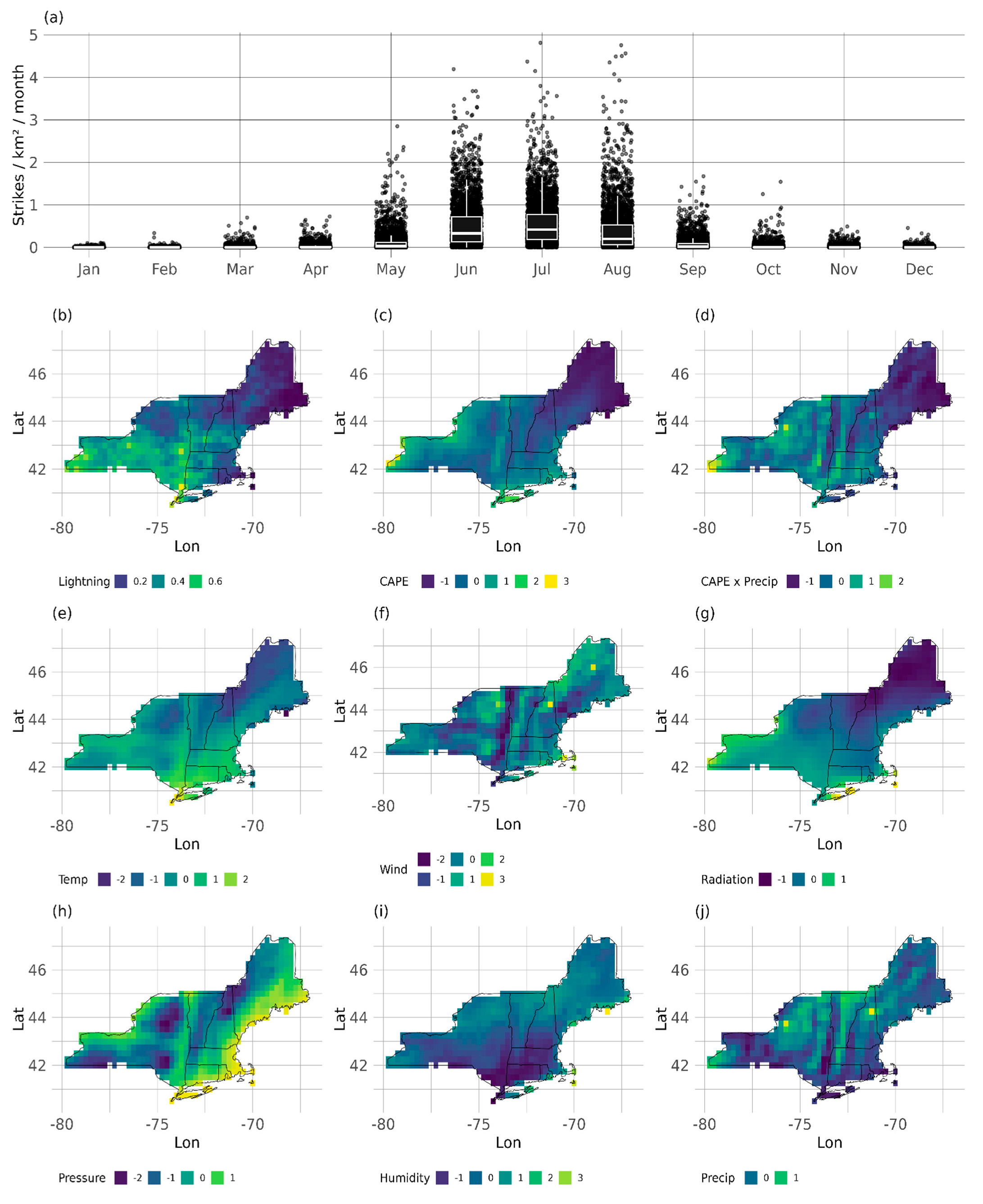
Figure 1. Spatial and temporal distribution of observed lightning and climate data. (a) Monthly distribution of lightning strike rates (strikes km−2 month−1) across the Northeastern United States for the period 2005–2010. Each dot represents the strike rate at a single grid point in a given month across all years in the study period. To improve visibility, points are jittered along the x-axis. Overlaid box-and-whisker plots summarize the distribution in each month, showing the median (line), first and third quartiles (box), and whiskers extending to 1.5 times the interquartile range. (b) cloud-to-ground lightning strike rate (strikes/km2/month), (c) CAPE (J/kg), (d) CAPE × Precipitation (W/m2), (e) Temperature (Celsius), (f) Wind speed (m/s), (g) Short-wave radiation (W/m2), (h) Surface pressure (Pa), (i) Relative humidity (%), and (j) Precipitation (kg/m2/s). Mapped values are for summer months (May–September), averaged across the 2005–2010 training period. All variables excluding the target (lightning strike rate) are standardized. Lightning data are derived from the Vaisala Lightning Database and climate data come from the ERA5 climate reanalysis product (Vaisala, Inc., Tucson, AZ, USA; Hersbach et al., 2020 [27]).
Atmosphere 16 01298 g001
Figure 2. Comparison of performance across modeling approaches and predictor variables. (a) Normalized root mean squared error (nRMSE). (b) Correlation between observed and predicted values. (c) S-score. (d) Anomaly correlation coefficient (ACC). (e) Normalized root mean squared error of Anomalies (nRMSE of Anomalies). For all plots, the right-most points indicate the best performing model (the x-axis of plots (a,f) have been reversed to reflect this). The y-axis of each plot contains the climate variables that a given model predicts lightning strike rate from, including convective available potential energy (CAPE), CAPE × precipitation (CAPE × Pr), relative humidity (RH), shortwave radiation (Rsds), temperature (T), surface pressure (Ps), precipitation (Pr), and wind (U10). Color indicates modeling approach; see Table 1 for model descriptions and definitions. All metrics were calculated using the test data [27,28].
Atmosphere 16 01298 g002
Figure 3. Variable importance from the random forest analysis predicting lightning strike rates. Importance is quantified as (a) the percentage increase in mean squared error (% Increase in MSE) when each predictor is permuted and (b) the total node impurity (measured by the Gini index) attributed to each predictor across all trees. Higher values indicate greater predictor influence. Predictors include shortwave radiation (Rsds), surface pressure (Ps), relative humidity (RH), wind (U10), temperature (T), and precipitation (Pr).
Atmosphere 16 01298 g003
Figure 4. Density plots of model predictions and residuals. (a) Kernel density estimates (KDE) of lightning strike rate, with color and line type representing observed lightning strike rate (red) and lightning strike rates predicted from models N13, G13, and B12. Negative strike rates are a result of KDE smoothing. (b) KDE of residuals (observed—predicted lightning strike rate) for models N13, G13, and B12. Models N13 and G13 simulate lightning from six near-surface climate variables: relative humidity, shortwave radiation, temperature, surface pressure, precipitation, and wind. B12 excludes surface pressure.
Atmosphere 16 01298 g004
Figure 5. Spatial comparison of observed and predicted lightning strike rates. Raster cells are colored by lightning strike rate (strikes/km2/month) averaged across six summers (2005–2010) of observed data and predictions from models N13, G13, and B12. See Table 1 for model descriptions and definitions. All data are from the test set; white raster cells indicate latitude/longitude points not included in the test data due to the random splitting of the data into train (80%) and test (20%) sets.
Atmosphere 16 01298 g005
Figure 6. Observed versus predicted lightning strike rates. The dotted 1:1 line indicates perfect model performance. All axes are in units of lightning strikes/km2/month. The x-axis in each plot shows the observed strike rates, while the y-axes are predictions from (a) model N13, (b) model G13, and (c) model B12.
Atmosphere 16 01298 g006
Figure 7. Interannual variability of observed and predicted lightning strike rates in the Northeastern United States, 2005–2010. Symbols show annual mean strike rates for each model, with vertical bars indicating one standard deviation across grid cells. The black dotted line marks the 6-year observed mean. Colors and shapes distinguish models: observed lightning from the Vaisala Lightning Detection Network (red crosses); the CAPE-based model C1 from Chen et al. (2021) (yellow circles) [9]; the linear model N13 (purple triangles); the Gamma GLM G13 (magenta squares); and the Gamma Bayesian model B12 (orange diamonds). These models were chosen as representatives of each modeling approach (C, N, G, B) because they generally performed best across most evaluation metrics (see Figure 2).
Atmosphere 16 01298 g007
Table 1. Summary of model sets, including probability distribution, shorthand labels, predictor variables, and Interpretation of predictions.
Model SetProbability DistributionLabelPredictor Variable *Predictions
Baseline models (Chen et al., 2021 [9])Normal error, constant varianceC1–C5Upper-airExpected mean response
Linear modelNormal error, constant varianceN1–N2Upper-airExpected mean response
N3–N13Near-surface
Gamma GLMGamma-distributed errors, variance proportional to meanG1–G2Upper-airExpected mean response, always positive
G3–G13Near-surface
Gamma BayesianGamma distribution with full posterior uncertaintyB1–B2Upper-airFull predictive distribution accounting for uncertainty
B3–B13Near-surface
* Upper-air refers to CAPE and CAPE × precip, while near-surface refers to relative humidity, shortwave radiation, temperature, surface pressure, precipitation, and wind.
Table 2. Baseline model descriptions and parameter estimates.
Model Label Functional   Form   for   E [ r s ] ab
C1a(CAPE × Pr)b4.441 ± 0.3371.206 ± 0.069
C2a(CAPE × Pr)b15.090 ± 4.5960.794 ± 0.066
C3a(CAPE × Pr)32.753 ± 2.565NA *
C4Non-parametric modelNANA
C5Ensemble meanNANA
* NA values indicate models that do not include that parameter.
Table 3. Linear model descriptions and parameter estimates.
Model
Label
Functional   Form   for   E r s  1abcdefg
N1a + b × CAPE0.335 ± 0.0090.117 ± 0.009NA 2NANANANA
N2a + b × (CAPE × Pr)0.335 ± 0.0090.111 ± 0.009NANANANANA
N3a + b × RH0.335 ± 0.009−0.089 ± 0.009NANANANANA
N4a + b × Rsds0.335 ± 0.0090.114 ± 0.009NANANANANA
N5a + b × T0.335 ± 0.0090.095 ± 0.009NANANANANA
N6a + b × Ps0.335 ± 0.010−0.018 ± 0.010NANANANANA
N7a + b × Pr0.335 ± 0.010−0.024 ± 0.010NANANANANA
N8a + b × U100.335 ± 0.009−0.075 ± 0.009NANANANANA
N9a + b × Rsds + c × T0.335 ± 0.0090.089 ± 0.0100.044 ± 0.010NANANANA
N10a + b × Rsds + c × T + d × RH0.335 ± 0.0090.082 ± 0.0110.035 ± 0.012−0.021 ± 0.012NANANA
N11a + b × Rsds + c × T + d × RH + e × U100.335 ± 0.0080.087 ± 0.0110.014 ± 0.012−0.020 ± 0.011−0.056 ± 0.009NANA
N12a + b × Rsds + c × T + d × RH + e × U10 + f × Pr0.335 ± 0.0080.130 ± 0.0110.001 ± 0.011−0.060 ± 0.012−0.053 ± 0.0080.095 ± 0.011NA
N13a + b × Rsds + c × T + d × RH + e × U10 + f × Pr + g × Ps0.335 ± 0.0080.113 ± 0.0110.052 ± 0.013−0.027 ± 0.012−0.068 ± 0.0080.069 ± 0.011−0.071 ± 0.010
1 Climate predictors include convective available potential energy (CAPE), CAPE × precipitation, relative humidity (RH), shortwave radiation (Rsds), temperature (T), surface pressure (Ps), precipitation (Pr), and wind (U10). 2 NA values indicate models that do not include that parameter.
Table 4. Gamma GLM descriptions and parameter estimates.
Model LabelFunctional Form for E[rs] 1abcdefg
G1exp(a + b × CAPE)−1.168 ± 0.0280.444 ± 0.028NA 2NANANANA
G2exp(a + b × CAPE × Pr)−1.153 ± 0.0290.369 ± 0.029NANANANANA
G3exp(a + b × RH)−1.130 ± 0.027−0.267 ± 0.027NANANANANA
G4exp(a + b × Rsds)−1.151 ± 0.0260.337 ± 0.026NANANANANA
G5exp(a + b × T)−1.141 ± 0.0270.332 ± 0.027NANANANANA
G6exp(a + b × Ps)−1.096 ± 0.029−0.060 ± 0.029NANANANANA
G7exp(a + b × Pr)−1.097 ± 0.029−0.067 ± 0.029NANANANANA
G8exp(a + b × U10)−1.121 ± 0.028−0.236 ± 0.028NANANANANA
G9exp(a + b × Rsds + c × T)−1.164 ± 0.0260.246 ± 0.0320.195 ± 0.032NANANANA
G10exp(a + b × Rsds + c × T + d × RH)−1.164 ± 0.0260.244 ± 0.0330.193 ± 0.035−0.004 ± 0.035NANANA
G11exp(a + b × Rsds + c × T + d × RH + e × U10)−1.173 ± 0.0260.256 ± 0.0340.124 ± 0.0370.000 ± 0.035−0.150 ± 0.028NANA
G12exp(a + b × Rsds + c × T + d × RH + e × U10 + f × Pr)−1.197 ± 0.0260.382 ± 0.0370.077 ± 0.037−0.145 ± 0.038−0.150 ± 0.0270.305 ± 0.035NA
G13exp(a + b × Rsds + c × T + d × RH + e × U10 + f × Pr + g × Ps)−1.223 ± 0.0240.324 ± 0.0360.299 ± 0.042−0.017 ± 0.039−0.218 ± 0.0270.214 ± 0.036−0.313 ± 0.032
1 Climate predictors include convective available potential energy (CAPE), CAPE × precipitation, relative humidity (RH), shortwave radiation (Rsds), temperature (T), surface pressure (Ps), precipitation (Pr), and wind (U10). 2 NA values indicate models that do not include that parameter.
Table 5. Gamma Bayesian Model descriptions and parameter estimates.
Model LabelFunctional Form for α 1,3aαbαcαdαeαfαgα
B1aα + bα × CAPE2.631 ± 0.1361.156 ± 0.104NANANANANA
B2aα + bα × (CAPE × Pr)2.474 ± 0.1321.060 ± 0.108NANANANANA
B3aα + bα × RH1.860 ± 0.0930.007 ± 0.013NANANANANA
B4aα + bα × Rsds2.108 ± 0.1060.604 ± 0.059NANANANANA
B5aα + bα × T2.054 ± 0.1060.549 ± 0.056NANANANANA
B6aα + bα × Ps1.699 ± 0.0860.007 ± 0.014NANANANANA
B7aα + bα × Pr1.713 ± 0.0850.120 ± 0.083NANANANANA
B8aα + bα × U101.818 ± 0.0910.006 ± 0.012NANANANANA
B9aα + bα × Rsds + cα × T2.204 ± 0.1150.103 ± 0.1060.458 ± 0.106NANANANA
B10aα + bα × Rsds + cα × T + dα × RH2.208 ± 0.1130.127 ± 0.1150.503 ± 0.1130.094 ± 0.120NANANA
B11aα + bα × Rsds + cα × T + dα × RH + eα × U102.390 ± 0.1320.204 ± 0.1280.394 ± 0.1370.089 ± 0.130−0.186 ± 0.096NANA
B12exp(aα + bα × Rsds + cα × T + dα × RH + eα × U10 +fα × Pr)0.970 ± 0.0500.276 ± 0.0770.009 ± 0.085−0.144 ± 0.078−0.172 ± 0.0570.303 ± 0.073NA
B13exp(aα + bα × Rsds + cα × T + dα × RH + eα × U10 +fα × Pr + gα × Ps1.096 ± 0.0510.181 ± 0.0800.174 ± 0.0980.028 ± 0.088−0.265 ± 0.0610.128 ± 0.077−0.281 ± 0.071
Model LabelFunctional Form for β 2,3aβbβcβdβeβfβgβ
B1aβ + bβ × CAPE7.552 ± 0.4150.683 ± 0.282NA 4NANANANA
B2aβ + bβ × CAPE × Pr7.116 ± 0.4110.654 ± 0.287NANANANANA
B3aβ + bβ × RH5.860 ± 0.3311.291 ± 0.151NANANANANA
B4aβ + bβ × Rsds6.247 ± 0.3550.020 ± 0.039NANANANANA
B5aβ + bβ × T6.080 ± 0.3510.049 ± 0.088NANANANANA
B6aβ + bβ × Ps5.063 ± 0.2980.295 ± 0.152NANANANANA
B7aβ + bβ × Pr5.141 ± 0.2970.714 ± 0.284NANANANANA
B8aβ + bβ × U105.664 ± 0.3251.212 ± 0.167NANANANANA
B9aβ + bβ × Rsds + cβ × T6.849 ± 0.394−1.282 ± 0.3290.403 ± 0.344NANANANA
B10aβ + bβ × Rsds + cβ × T + dβ × RH6.880 ± 0.386−1.136 ± 0.3540.706 ± 0.3780.571 ± 0.360NANANA
B11aβ + bβ × Rsds + cβ × T + dβ × RH + eβ × U107.601 ± 0.469−1.138 ± 0.4040.695 ± 0.4580.559 ± 0.4050.622 ± 0.325NANA
B12exp(aβ + bβ × Rsds + cβ × T + dβ × RH + eβ × U10 + fβ × Pr)2.163 ± 0.056−0.102 ± 0.083−0.052 ± 0.0890.001 ± 0.094−0.020 ± 0.0660.026 ± 0.083NA
B13exp(aβ + bβ × Rsds + cβ × T + dβ × RH + eβ × U10 + fβ × Pr + gβ×Ps)2.312 ± 0.056−0.132 ± 0.082−0.079 ± 0.1050.085 ± 0.097−0.061 ± 0.069−0.087 ± 0.083−0.020 ± 0.083
1 α is the shape parameter of the gamma distribution. 2 β is the scale parameter of the gamma distribution. 3 Climate predictors include convective available potential energy (CAPE), CAPE × precip (CAPE × Pr), relative humidity (RH), shortwave radiation (Rsds), temperature (T), surface pressure (Ps), precipitation (Pr), and wind (U10). 4 NA values indicate models that do not include that parameter.
Disclaimer/Publisher’s Note: The statements, opinions and data contained in all publications are solely those of the individual author(s) and contributor(s) and not of MDPI and/or the editor(s). MDPI and/or the editor(s) disclaim responsibility for any injury to people or property resulting from any ideas, methods, instructions or products referred to in the content.