Modeling Tropical Cyclone Boundary Layer Wind Fields over Ocean and Land: A Comparative Assessment

Abstract

Accurate simulation of boundary layer wind field structures is essential for evaluating tropical cyclone (TC) wind hazards and supporting engineering design in coastal regions. However, existing models often assume radially symmetric and homogeneous surface conditions, leading to limited accuracy near landfall where surface roughness varies significantly. This study conducts a comprehensive evaluation of four representative TC boundary layer models of M95, K01, Y21a, and Y21b, under both idealized and real TC case conditions. The idealized experiments are used to clarify the role of vertical advection and turbulent diffusion in shaping the TC boundary layer, while the landfalling case of Typhoon Mangkhut (2018) is simulated to examine the impacts of surface roughness parameterization. Results show that Y21a, which incorporates nonlinear vertical advection, produces stronger and more realistic super-gradient phenomenon than linear models of M95 and K01. Furthermore, the model of Y21b, which accounts for spatially varying drag coefficients and using a terrain-following coordinate system, successfully reproduces the asymmetric wind patterns observed in the WRF simulations during landfall, achieving the highest correlation (R = 0.93). When the spatially varying drag coefficients incorporated into the linear models, their correlation with WRF improved markedly by about 37%. These findings highlight the necessity of incorporating nonlinear advection, dynamic turbulence, and surface heterogeneity for physically consistent TC boundary layer simulations. The results provide valuable guidance for improving parametric wind field models and enhancing TC wind hazard assessments over complex coastal terrains.

1. Introduction

Tropical cyclone (TC) is one of the most destructive weather systems on Earth. It can produce strong winds, heavy rainfall, and storm surge that severely threaten both coastal and inland communities [1,2,3]. As a TC approaches land, it encounters a different low boundary environment, which is characterized by reduced moisture availability and enhanced surface roughness compared with the open ocean [4,5]. The transition from the smooth, thermally uniform oceanic surface to the heterogeneous land surface significantly changes the TC boundary layer dynamics, leading to a rapid weakening of TC wind speeds [6]. The process of TC decay after landfall can be attributed to the loss of the oceanic heat source and it has been extensively documented in both observational [7,8] and numerical studies [6,9].

However, less attention has been devoted to investigating the role of surface friction asymmetry in modifying parametric wind field model simulations. Early studies, such as those by Tuleya and Kurihara [10] and Powell [11], recognized that frictional effects are essential in shaping the asymmetric wind structure for landfalling TCs. The enhanced surface roughness over land increases the drag effects of boundary layer, resulting in a stronger inflow and a subsequent redistribution of angular momentum within the eyewall. Later analytical studies [12,13] further clarified the boundary layer dynamics that produce spatial asymmetries.

Despite these studies, parametric models, such as those proposed by Holland [14] and Willoughby and Rahn [15], assume radial symmetry and neglect the land-induced variability in surface roughness. Such simplification may be acceptable for TCs over the open ocean, where surface properties are horizontally homogeneous, but it becomes problematic when the TC approaches coastal or complex terrains. As a result, these models often underestimate wind asymmetry and overestimate wind magnitude, leading to biases in hazard assessments and engineering design applications [16,17]. Simulations using mesoscale models such as the Weather Research and Forecasting (WRF) model reveal that land-induced frictional asymmetry can lead to significant azimuthal variations in wind speed and vertical motion [18,19]. Specifically, the rougher land surface enhances turbulent mixing and reduces near-surface wind speeds locally, while the associated inflow asymmetry induces shifts in the eyewall convection and surface wind maxima. Therefore, the structure of landfalling TCs cannot be fully simulated without considering the coupled effects of surface heterogeneity and boundary layer dynamics.

In recent years, several advanced parametric TC boundary layer models have been developed to incorporate spatially varying surface drag coefficients that account for land cover and topographic variations [20,21,22]. These models extend beyond the traditional axisymmetric framework, enabling a more realistic representation of asymmetric inflow, momentum exchange, and turbulence generation. For instance, Yang, et al. [20] adopted a terrain-following coordinate system based on the formulation of Tzvi and Somerville [23], allowing the model to capture the land–sea transition and surface roughness effects more accurately. This modification significantly improves agreement between simulated and WRF-derived wind fields, demonstrating the potential benefits of incorporating spatially heterogeneous boundary conditions into parametric TC models. Moreover, the dynamic processes of horizontal advection, vertical advection, and vertical diffusion are further incorporated into parametric TC models to better simulate the vertical structure characteristics of TCs, such as the super-gradient wind, a common feature in TC boundary layers. By using a full-physics model, Fei, et al. [24] found that the removal of vertical advection reduces both the strength and height of super-gradient wind by about 50%. Then, Snaiki and Wu [25] refined an analytical parametric model to account for the effects of vertical advection. Their results showed that the maximum super-gradient wind is about 10% higher than gradient wind speed when vertical advection was included, but only about 5% higher when it was not.

However, systematic evaluations of how these advanced boundary layer formulations perform under both oceanic and landfalling conditions remain limited. Understanding and accurately modeling asymmetry TC wind field is not only a matter of academic interest but also of practical significance. The asymmetric distribution of surface winds directly influences the design of offshore structures, such as wind turbines that are primarily affected by strong winds [26,27], as well as floating structures that are susceptible to heavy waves [28,29]. Furthermore, as climate change may alter coastal land cover and urban roughness patterns, improved representation of frictional effects in parametric TC models becomes increasingly critical for future risk assessment and disaster mitigation.

Therefore, the aims of this study are as follows: (1) to advance the understanding of how surface roughness affects the structure of TC wind fields; (2) to conduct a comprehensive intercomparison of four representative TC boundary layer models (Meng, et al. [30] (M95), Kepert [12] (K01), Yang, et al. [31] (Y21a), and Yang, et al. [20] (Y21b)); and (3) to examine the performance of these models across both oceanic and landfalling conditions. By comparing models’ performance under idealized and real TC cases, this study systematically investigates the roles of vertical advection, turbulent diffusion, and surface roughness parameterization in shaping the TC boundary layer structures. Particular attention is given to quantifying model improvements over land and to assess how the incorporation of spatially varying drag coefficients enhances the realism of simulated wind fields. The remainder of this paper is organized as follows. Section 2 introduces the gradient wind model and the four selected TC boundary layer wind field models, together with the method used to represent land surface roughness. Section 3 presents and compares the results of both idealized and real TC simulations. Section 4 provides further discussion of the findings and outlines the limitations of the study. Section 5 summarizes the main conclusions of this work.

2. Parametric TC Wind Field Models

2.1. Gradient Wind Field Model

According to the TC vertical wind profiles measured by GPS dropsondes, Giammanco, et al. [32] found that the region approximately 300–800 m above the ground surface constitutes the inflow layer of a TC. Within this layer, the underlying surface (such as terrain, landcover, etc.) exerts a significant influence on the TC wind field. With the increase in height, the impact of surface conditions gradually diminishes and can eventually be ignored above the top of the TC boundary layer. Beyond this height, the gradient wind, free from surface influence, can be approximately established based on the empirical expressions or the gradient wind balance.

One of the most widely used gradient wind models was proposed by Holland [14], which formulates the wind structure based on the balance among the pressure gradient force, the Coriolis force, and the centrifugal force. Other models, such as that of Willoughby, et al. [33], divide the wind field into three regions (inside the eye wall, outside the eye wall, and the transition zone between them) to generate the TC gradient wind field. According to the study of Holland [14], the gradient wind field (v_g) of a moving TC in a cylindrical coordinate system (r, λ, z) can be expressed as,

$$v_g\left(r,\lambda \right)=-{\displaystyle \frac{v_{c,\lambda }+f\cdot r}{2}}+\sqrt{{\left({\displaystyle \frac{v_{c,\lambda }+f\cdot r}{2}}\right)}^2+{\displaystyle \frac{r}{{\rho }_0}}{\displaystyle \frac{\mathsf{\partial }p}{\mathsf{\partial }r}}},$$

(1)

$$p=p_c+∆p\cdot exp\left[-{\left({\displaystyle \frac{R_{max}}{r}}\right)}^B\right],$$

(2)

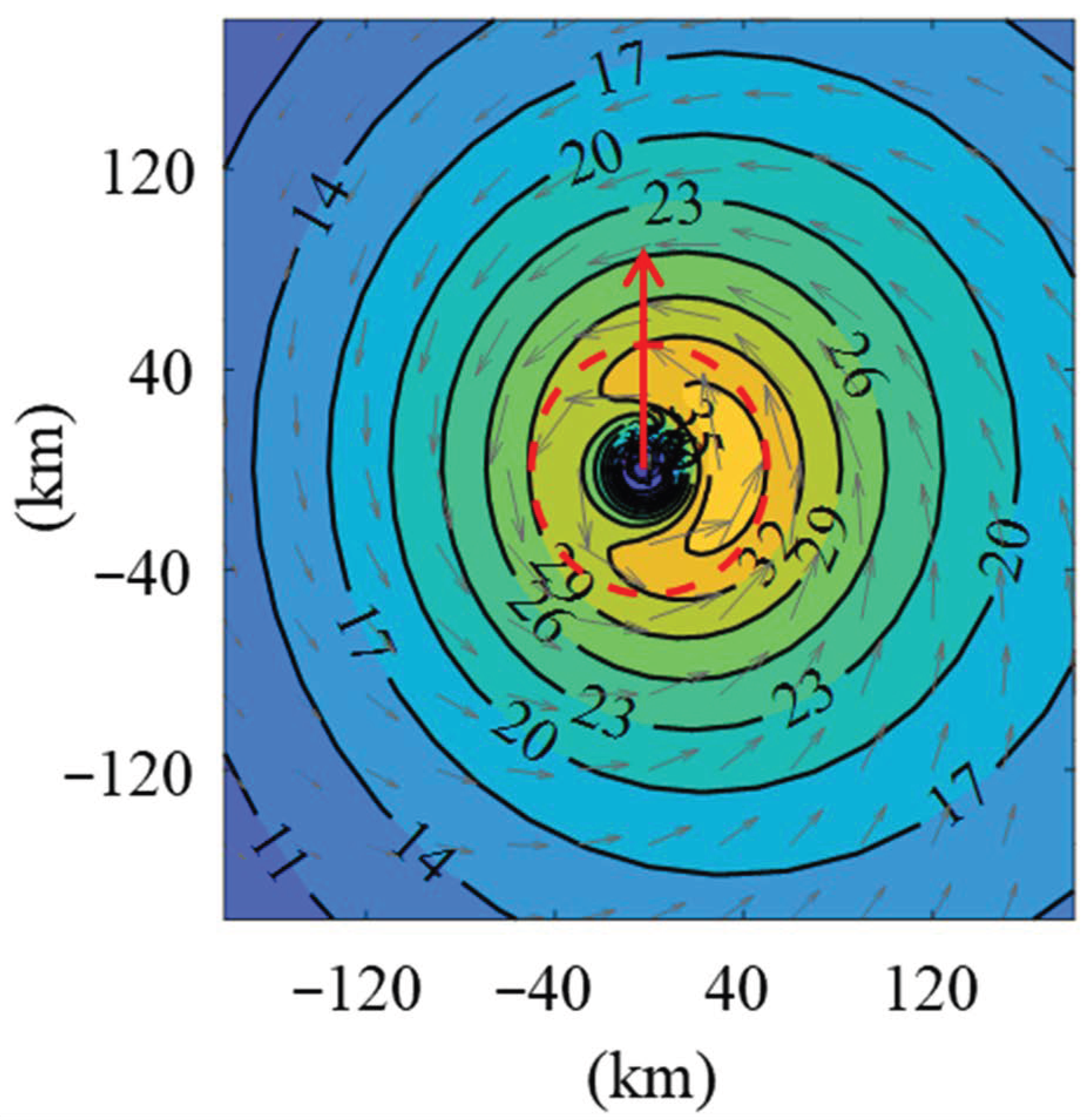
in which v_c,λ (m/s) is the tangential component of the TC moving velocity; f (s⁻¹) is the Coriolis parameter; r (m) is the radius distance from the TC center; ρ₀ (kg/m³) is the air density (commonly taken as 1.15 kg/m³); p (Pa) is the atmospheric pressure; p_c (Pa) is the TC center pressure; ∆p (Pa) is the pressure deficit defined as the difference between p_c and the reference atmospheric pressure (1010 hPa is adopted); R_max (m) is the radius of maximum wind; B is the shape parameter of TC pressure profile. Figure 1 shows the gradient field of a TC case.

Figure 1. Gradient wind field calculated from Equation (1). The maximum gradient wind speed is 40 m/s at R_max = 40 km with a shape parameter B = 1.3. The TC translates northward at 5 m/s, with a center pressure of 969.61 hPa. The red arrow indicates the TC moving direction, gray arrows denote wind directions, and the red dashed line denotes R_max. This gradient wind field is identical to that of TC II in Yang, et al. [20] and is used in this study as the upper boundary condition for model comparisons that is carried out in Section 3.1.

For engineering applications, the gradient wind should be adjusted from the top of the atmospheric boundary layer to the near-surface level (typically the height of 10 m). Georgiou, et al. [34] suggested that the reduction factor should vary with the TC radius, taking a value of 0.845 at the radius of maximum wind and 0.68 in the outer region of a TC. Batts, et al. [35] approximated the factor as 0.865 over ocean and 0.85 over land. More recently, Du, et al. [36] adopted a constant value of 0.85 to convert gradient winds to ocean-surface to drive storm surge model. Although different studies have employed varying coefficients, most values fall within the range of 0.67–0.87, as shown in Table 1. Furthermore, Kepert [12] demonstrated that the spatial distribution of the reduction factor in a TC over ocean is not uniform, being larger in regions of stronger winds and smaller where winds are weaker. These findings indicate that applying a single reduction factor, which has been used by many studies [16,37], may lead to inaccuracies in estimating near-surface TC wind speeds, thereby underscoring the necessity of more physically based TC boundary layer models.

Table 1. Reported reduction factors for converting gradient wind speed to sea-surface (10 m) wind speed in different studies.

	Batts, et al. [35]	Georgiou [38]	Vickery, et al. [39], Vickery, et al. [40]	Sparks and Huang [41]	Powell, et al. [42]	Powell, et al. [43]	Vickery, et al. [44]
Reduction factor	0.865	0.825 (0.5 Rmax < r < 2 Rmax), 0.75 (r > 5 Rmax)	0.7–0.72	0.65	0.71	0.73	0.67–0.74

2.2. Four Selected TC Boundary Layer Models

In this study, four parametric TC boundary layer models of Meng, et al. [30], Kepert [12], Yang, et al. [31], and Yang, et al. [20] that have been previously applied in the Northwestern Pacific Ocean are selected for evaluation. A number of other models (e.g., Hong, et al. [22], Shapiro [45], Thompson and Cardone [46], Kepert and Wang [47], Snaiki and Wu [48], Fang, et al. [49]) have also been proposed and applied in TC wind hazard analysis, storm surge simulation, and TC rainfall forecasting. The four models investigated here are chosen for their differing assumptions and simplifications of the governing dynamic equations, their reproducibility, their alignment with the authors’ previous research experience.

Parametric TC wind field models are generally designed to estimate TC wind fields according to the conditions at the top of the boundary layer, which typically derived from the gradient wind field (e.g., Equation (1)) or the TC pressure field (e.g., Equation (2)). Then, the TC wind fields are simulated by solving the dynamic equations with prescribed parameterizations of turbulent exchange and surface friction. The main differences among the models are the assumptions and approximations adopted to simplify the governing equations, as well as the numerical or analytical solution methods employed. As stated in Kepert [4], these parametric models assume that the gradient wind field is known and remains constant in time. Consequently, there is no feedback from the boundary layer to the cyclone, and the simulations represent only a “steady” wind field. Nevertheless, such models remain widely used in both research and engineering applications because of their computational efficiency and their ability to approximate boundary layer wind fields. A systematic evaluation of their performance, particularly in simulating landfalling TCs where surface roughness exhibits strong spatial variability, is therefore crucial for clarifying their applicability to TC hazard assessment. The four models (M95, K01, Y21a, and Y21b) considered in this study are described below.

2.2.1. The Model of M95

The model of M95 [30] is a height-resolving TC boundary layer model that represents wind speed as the sum of the gradient wind (v_g) and the friction-caused wind (v′). In this model, governing dynamic equations are simplified by using the scale analysis approach in a cylindrical coordinate system (r, λ, z), and written as,

$$-\left({\displaystyle \frac{2v_g}{r}}+f\right)v^{\prime }=K_V{\displaystyle \frac{{\mathsf{\partial }}^2{u}^{\prime }}{\mathsf{\partial }{z}^2}},$$

(3)

$$\left({\displaystyle \frac{\mathsf{\partial }{v}_g}{\mathsf{\partial }r}}+{\displaystyle \frac{v_g}{r}}+f\right)u^{\prime }=K_V{\displaystyle \frac{{\mathsf{\partial }}^2{v}^{\prime }}{\mathsf{\partial }{z}^2}},$$

(4)

in which u′ and v′ are the radial and tangential components of v′, respectively; K_V is the vertical eddy viscosity coefficient and can be taken as fixed value such as 100 m²/s [30] or 50 m²/s [12]. The TC boundary layer wind components (u, v) are then obtained as,

$$u=u_g+u^{\prime }+u_{c,r},$$

(5)

$$v=v_g+v^{\prime }+v_{c,\lambda },$$

(6)

where u_g and v_g are the radial and tangential components of v_g, respectively; u_c,r and v_c,λ are the radial and tangential components of TC moving velocity, respectively. To account for land cover effects, M95 further incorporates a surface boundary condition in which the shearing stress is balanced by the surface drag force,

$$K_V{{\displaystyle \frac{\mathsf{\partial }\left(u,v\right)}{\mathsf{\partial }z}}}_{z\to 0}=C_d\sqrt{u^2+v^2}\cdot \left(u,v\right),$$

(7)

where C_d is the drag coefficient. The model of M97 explicitly resolves the vertical structure of the boundary layer, thereby providing a more detailed representation of TC wind fields.

2.2.2. The Model of K01

Similarly to M95, which divides the TC wind into v_g and v′, Kepert [12] (abbreviated as K01) proposed a linear analytical model that additionally incorporates the tangential advection (v_g/r∙∂(u′, v′)/∂λ) within the TC boundary layer. In the cylindrical coordinate system (r, λ, z), the governing equations are expressed as,

$${\displaystyle \frac{v_g}{r}}{\displaystyle \frac{\mathsf{\partial }{u}^{\prime }}{\mathsf{\partial }\lambda }}-\left({\displaystyle \frac{2v_g}{r}}+f\right)v^{\prime }=K_V{\displaystyle \frac{{\mathsf{\partial }}^2{u}^{\prime }}{\mathsf{\partial }{z}^2}},$$

(8)

$${\displaystyle \frac{v_g}{r}}{\displaystyle \frac{\mathsf{\partial }{v}^{\prime }}{\mathsf{\partial }\lambda }}+\left({\displaystyle \frac{\mathsf{\partial }{v}_g}{\mathsf{\partial }r}}+{\displaystyle \frac{v_g}{r}}+f\right)u^{\prime }=K_V{\displaystyle \frac{{\mathsf{\partial }}^2{v}^{\prime }}{\mathsf{\partial }{z}^2}}.$$

(9)

In K01, the TC wind field is represented as the sum of the following three components: one axisymmetric flow and two asymmetric flows (fourier wavenumber of 0 and ±1). The axisymmetric component is primarily determined by TC dynamics, while the asymmetric components are generated through the interaction between TC movement and the underlying surface. However, the linearization method used in K01 ignores some terms whose magnitude is not negligible. For example, the vertical advection terms (w∙∂(u, v)/∂z) are comparable to the vertical diffusion in the eyewall region (Figure 5 in Yang, et al. [31]) and should not be eliminated. Compared with M95, the inclusion of tangential linear inflows in K01 results in a more mixed wind field, with a slightly weaker jet strength than that produced by M95. The simulated jet strength in K01 and M95 is about 1.03 at R_max, whereas observations of Giammanco, et al. [32] indicate a value of about 1.1. This discrepancy primarily arises because vertical advection and nonlinear radial advection are not explicitly represented in these models.

2.2.3. The Model of Y21a

Based on the study of M97 and K01, Yang, et al. [31] (abbreviated as Y21a) developed a height-resolving TC boundary layer model to further consider the effect of vertical advection process and the model formulated as

$${\displaystyle \frac{v_g}{r}}{\displaystyle \frac{\mathsf{\partial }{u}^{\prime }}{\mathsf{\partial }\lambda }}-({\displaystyle \frac{2v_g}{r}}+f)v^{\prime }+w^{\prime }{\displaystyle \frac{\mathsf{\partial }{u}^{\prime }}{\mathsf{\partial }z}}=K_V{\displaystyle \frac{{\mathsf{\partial }}^2{u}^{\prime }}{\mathsf{\partial }{z}^2}},$$

(10)

$${\displaystyle \frac{v_g}{r}}{\displaystyle \frac{\mathsf{\partial }{v}^{\prime }}{\mathsf{\partial }\lambda }}+({\displaystyle \frac{\mathsf{\partial }{v}_g}{\mathsf{\partial }r}}+{\displaystyle \frac{v_g}{r}}+f)u^{\prime }+w^{\prime }{\displaystyle \frac{\mathsf{\partial }{v}^{\prime }}{\mathsf{\partial }z}}=K_V{\displaystyle \frac{{\mathsf{\partial }}^2{v}^{\prime }}{\mathsf{\partial }{z}^2}},$$

(11)

$$w=-{\displaystyle \frac{1}{r}}\left[{\displaystyle {\int }_0^z\frac{\mathsf{\partial }\left(ru\right)}{\mathsf{\partial }r}dz+{\displaystyle {\int }_0^z\frac{\mathsf{\partial }v}{\mathsf{\partial }\lambda }dz}}\right].$$

(12)

As shown in the governing equations, linear horizontal advection, nonlinear vertical advection, and nonlinear vertical diffusion are explicitly incorporated. Specially, u′ and v′ are solved analytically using Fourier transformation, while w is iteratively calculated from the continuity equation using numerical method. The inclusion of vertical advection enables Y21a to produce a jet strength of about 1.06 for stationary TCs and 1.08 for moving TCs, which is notably stronger than that of K01 (about 1.027 for both stationary and moving TCs) and M95 (about 1.035 for both conditions). Furthermore, the effect of vertical advection is relatively small near the lower boundary, but it becomes increasingly significant at higher levels, particularly above 100 m, which is a critical height for wind turbine hazard analysis under TC conditions. For landfalling TCs, Y21a combines the well-mixed boundary-layer theory with the flux-gradient theory (Holton, 2007) [50], providing a more physically consistent treatment of surface-atmosphere interactions.

2.2.4. The Model of Y21b

In contrast to the three aforementioned analytical models, which simplify and solve the governing equations through different assumptions, nonlinear models that retain more dynamic processes and employ more sophisticated parameterization schemes of turbulent have been proposed [20,21,47]. These models require time integration to reach a near-steady state, with the three-dimensional TC wind fields generated by solving the governing equations using a finite-difference scheme. The model of Yang, et al. [20] (abbreviated as Y21b) is constructed on a terrain-following coordinate system, which allows it to account for the effects of land cover and complex terrain. The governing equations of Y21b are formulated in the Cartesian coordinate system and expressed as follows,

$${\displaystyle \frac{du}{dt}}=-{\displaystyle \frac{1}{\rho }}{\displaystyle \frac{\mathsf{\partial }p}{\mathsf{\partial }x}}-f\cdot \left(v+v_{c,y}\right)+{\displaystyle \frac{\mathsf{\partial }}{\mathsf{\partial }x}}\left(K_H{\displaystyle \frac{\mathsf{\partial }u}{\mathsf{\partial }x}}\right)+{\displaystyle \frac{\mathsf{\partial }}{\mathsf{\partial }y}}\left(K_H{\displaystyle \frac{\mathsf{\partial }u}{\mathsf{\partial }y}}\right)+{\displaystyle \frac{\mathsf{\partial }}{\mathsf{\partial }z}}\left(K_V{\displaystyle \frac{\mathsf{\partial }u}{\mathsf{\partial }z}}\right),$$

(13)

$${\displaystyle \frac{dv}{dt}}=-{\displaystyle \frac{1}{\rho }}{\displaystyle \frac{\mathsf{\partial }p}{\mathsf{\partial }y}}-f\cdot \left(u+u_{c,x}\right)+{\displaystyle \frac{\mathsf{\partial }}{\mathsf{\partial }x}}\left(K_H{\displaystyle \frac{\mathsf{\partial }v}{\mathsf{\partial }x}}\right)+{\displaystyle \frac{\mathsf{\partial }}{\mathsf{\partial }y}}\left(K_H{\displaystyle \frac{\mathsf{\partial }v}{\mathsf{\partial }y}}\right)+{\displaystyle \frac{\mathsf{\partial }}{\mathsf{\partial }z}}\left(K_V{\displaystyle \frac{\mathsf{\partial }v}{\mathsf{\partial }z}}\right),$$

(14)

$${\displaystyle \frac{\mathsf{\partial }u}{\mathsf{\partial }x}}+{\displaystyle \frac{\mathsf{\partial }v}{\mathsf{\partial }y}}+{\displaystyle \frac{\mathsf{\partial }w}{\mathsf{\partial }z}}=0.$$

(15)

in which d/dt = ∂/∂t + u_c,x∙∂/∂x + v_c,y∙∂/∂y + u ∂/∂x + v∙∂/∂y + w∙∂/∂z; K_H is the horizontal diffusion coefficient, calculated following Thompson and Cardone [46]; K_V is estimated using the neutral-stability first-order Louis turbulent transport parameterization scheme that is recommended by Kepert [21]. The model is configured with a nested horizontal grid system, with the innermost grid spacing set to 0.1·R_max to resolve critical TC features near the center. The vertical grid consists of 20 levels, extending from 10 m above the surface to approximately 2.5 km, allowing the model to capture the full depth of the TC boundary layer while maintaining computational efficiency. This configuration, combined with explicit treatment of horizontal and vertical advection, vertical diffusion, and turbulent fluxes, enables Y21b to produce a physically consistent three-dimensional representation of TC boundary-layer winds.

2.3. Simulation Setups

2.3.1. Grid Systems

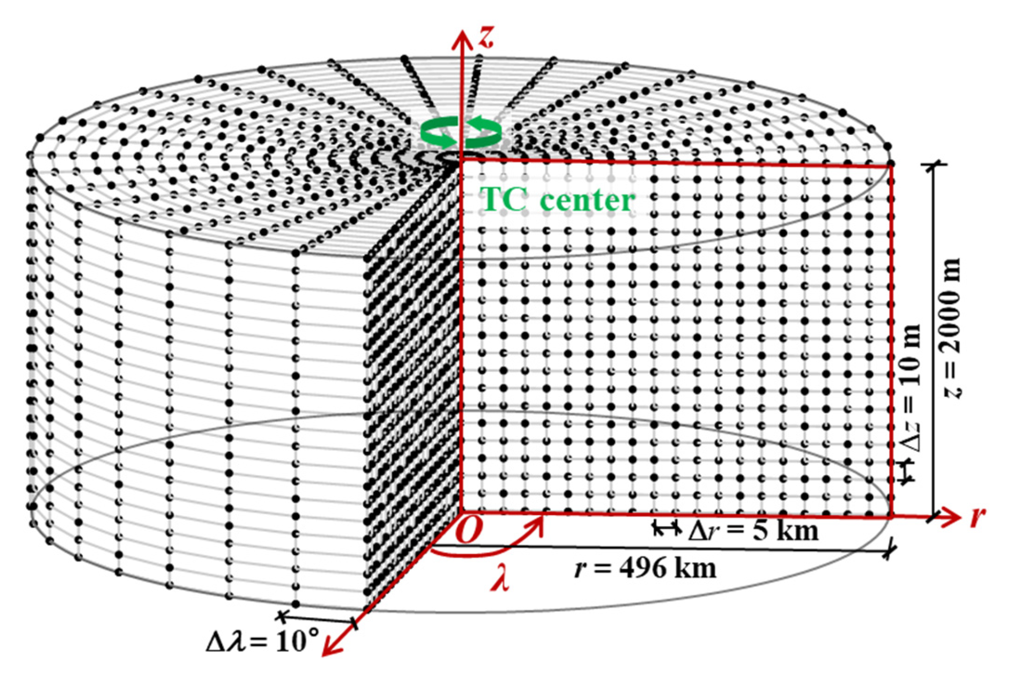
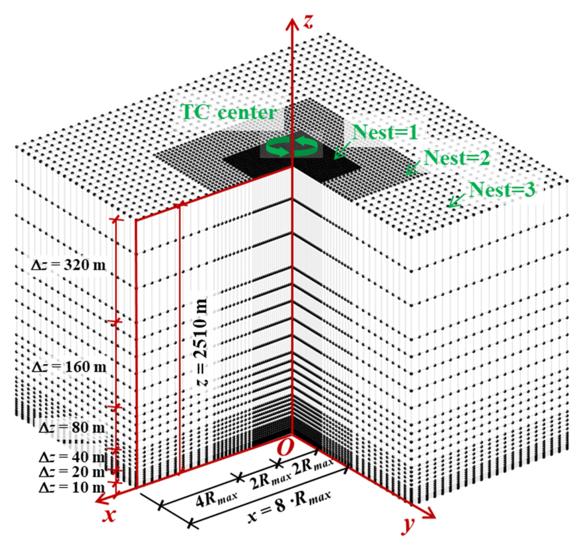
Based on the governing equations employed in the four selected models, two different grid systems are adopted for the simulations, as illustrated in Figure 2 and Figure 3. The cylindrical grid system (shown in Figure 2) is applied in M95, K01, and Y21a. The dynamic characteristics of TCs indicate that (1) the wind speed changes rapidly in the radial direction around TC eyewall, while it changes relatively slower in the tangential direction; and (2) the wind speed gradually decreases with the increase in radius beyond the eyewall region. Therefore, the grid system is designed with high spatial resolution near the eyewall and lower resolution in the outer region. In this study, TC center is located at the coordinate origin (O), and the cylindrical grid system is set as axisymmetric, consisting of 36 vertical planes along radial directions, with an angular spacing of 10° between two adjacent vertical planes. Within each vertical plane, the radial grid extends from 1 km to 496 km with a resolution of 5 km, while the vertical grid extends from 10 m to 2000 m with a resolution of 10 m.

Figure 2. Cylindrical grid system used in the models of M95, K01, and Y21a. The radial grid r ranges from 1 km to 496 km with 5 km resolution; the vertical grid z spans from 10 m to 2000 m with 10 m resolution; and the azimuthal grid λ ranges from 0° to 350° with 10° resolution. The TC center is located at the coordinate origin (O). Red arrows indicate the direction of the coordinate axis. Bold green arrows are the rotation direction of the TC wind field.

Figure 3. Cartesian three-level-nested grid system used in the model of Y21b. The horizontal coordinate x and y ranges from 0.1·R_max to 8·R_max, while the vertical coordinate z spans from 10 m to 2510 m. The TC center is located at the coordinate origin (O). Red arrows indicate the direction of the coordinate axis. Bold green arrows are the rotation direction of the TC wind field.

The cartesian nested grid system (shown in Figure 3) is applied in Y21b. To improve computational efficiency, the grid system is designed with higher resolution in the inner and lower regions of TC computation domain, and low resolution in the outer and upper regions. Specifically, a three-level nested horizontal grid system is applied. The grid spacing remains uniform within each nest and the spacing of the outer nest is twice that of the adjacent inner nest. Each nest consists of 20 grid points from the TC center. The grid spacing in the innermost nest is set as 0.1·R_max, while the second and third nests use 0.2·R_max and 0.4·R_max, respectively. The entire computational domain spans 16·R_max × 16·R_max on the horizontal. In the vertical direction, 28 layers are configured, including 7 layers from 0 to 100 m (10, 20, 30, 40, 50, 70, 90 m), 14 layers from 100 to 1000 m (110, 130, 150, 190, 230, 270, 310, 350, 430, 510, 590, 670, 750, 910 m), and 7 layers above 1000 m (1070, 1230, 1390, 1550, 1870, 2190, 2510 m).

2.3.2. Modification for Landfall TC Wind Field Simulations

As a TC moves over the ocean, it can absorb energy from the latent heat released by the warm sea surface evaporation. Once landfall, this energy supply is interrupted, leading to rapid TC weakening. Differences between land and ocean surfaces also have significant effect on TC dynamics. The ocean surface is relatively smooth, offering minimal frictional resistance, thereby preserving the integrity of TC structure. However, the land surface, characterized by vegetation, urban structures, and complex terrain, exhibits much higher roughness that can induce strong frictional dissipation in the lower-level flow. Consequently, the wind field of a landfalling TC weakens non-uniformly, showing significant spatial heterogeneity. In TC wind field simulations, the drag coefficient (C_d) is used to represent momentum exchange between the underlying surface and atmospheric flows. C_d at the height of 10 m over the ocean can be expressed as follows [5],

$${10}^3{C}_d=\min \left[\max \left(1.2, 0.7+0.065\cdot v_{10}\right), 2.3\right],$$

(16)

in which v₁₀ is the wind speed at 10 m, while over the land, the fixed value of C_d = 7.54 × 10⁻³ is used, corresponding to a roughness length of 0.1 m. Furtherly, Kepert [4] suggested to represent C_d as a sinusoidal variation to consider the land–sea roughness difference, but this scheme still fails to reflect the spatial variations in land surface characteristics.

According to Meng, et al. [30], C_d can be estimated from the surface roughness length (z₀) as,

$$C_d={\displaystyle \frac{{\kappa }^2}{{\left\{\ln \left[\left(z_{10}+h-d\right)/z_0\right]\right\}}^2}}$$

(17)

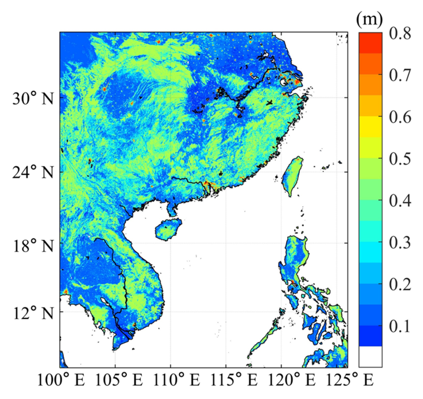
where κ is von Kärmän’s constant, taken as 0.4; h is the mean roughness-element height, calculated as h = 11.4·z₀^0.86; d is the zero-plane displacement, calculated as d = 0.75h; z₁₀ is the reference height of 10 m. Since z₀ is closely dependent on the physical properties of land cover, it can be estimated according to the land cover types within the simulation domain [51]. The Noah land surface model [52], which is widely employed in the regional and global weather forecasting models, parameterizes z₀ based on the land-class-based lookup table and time-series data. Therefore, this approach is adopted in the study to quantify z₀. Table 2 shows the land-class-based lookup table for z₀ applied in summer. The spatial distribution of z₀ over South Asia (shown in Figure 4) can be generated from the European Space Agency (ESA) Climate Change Initiative (CCI) global land cover dataset (the latest data version of CCI-LC 2020 with a spatial resolution of 300 m). As a result, the spatial heterogeneity of land surfaces can be incorporated into the TC wind field model via the drag coefficient C_d in Equation (17).

Table 2. Land-class-based lookup table for z₀ used in the Noah land surface model in summer.

Land Cover Types	z0	Land Cover Types	z0
Urban and built-up land	0.80	Mixed forest	0.50
Dryland cropland and pasture	0.15	Water bodies	0.0001
Irrigated cropland and pasture	0.10	Herbaceous wetland	0.20
Mixed dryland/irrigated cropland and pasture	0.15	Wooded wetland	0.40
Cropland/grassland mosaic	0.14	Baren or sparsely vegetated	0.01
Cropland/woodland mosaic	0.20	Herbaceous tundra	0.10
Grassland	0.12	Wooded tundra	0.30
Shrubland	0.05	Mixed tundra	0.15
Mixed shrubland/grassland	0.06	Bare ground tundra	0.10
Savanna	0.15	Snow or ice	0.001
Deciduous broadleaf forest	0.50	Playa	0.01
Deciduous needleleaf forest	0.50	Lava	0.15
Evergreen broadleaf forest	0.50	White sand	0.01
Evergreen needleleaf forest	0.50

Figure 4. Spatial distribution of surface roughness length (z₀) over South Asia, derived from the CCI-LC 2020 land cover data using the lookup table presented in Table 2.

3. Results

3.1. Idealized TC Case Study

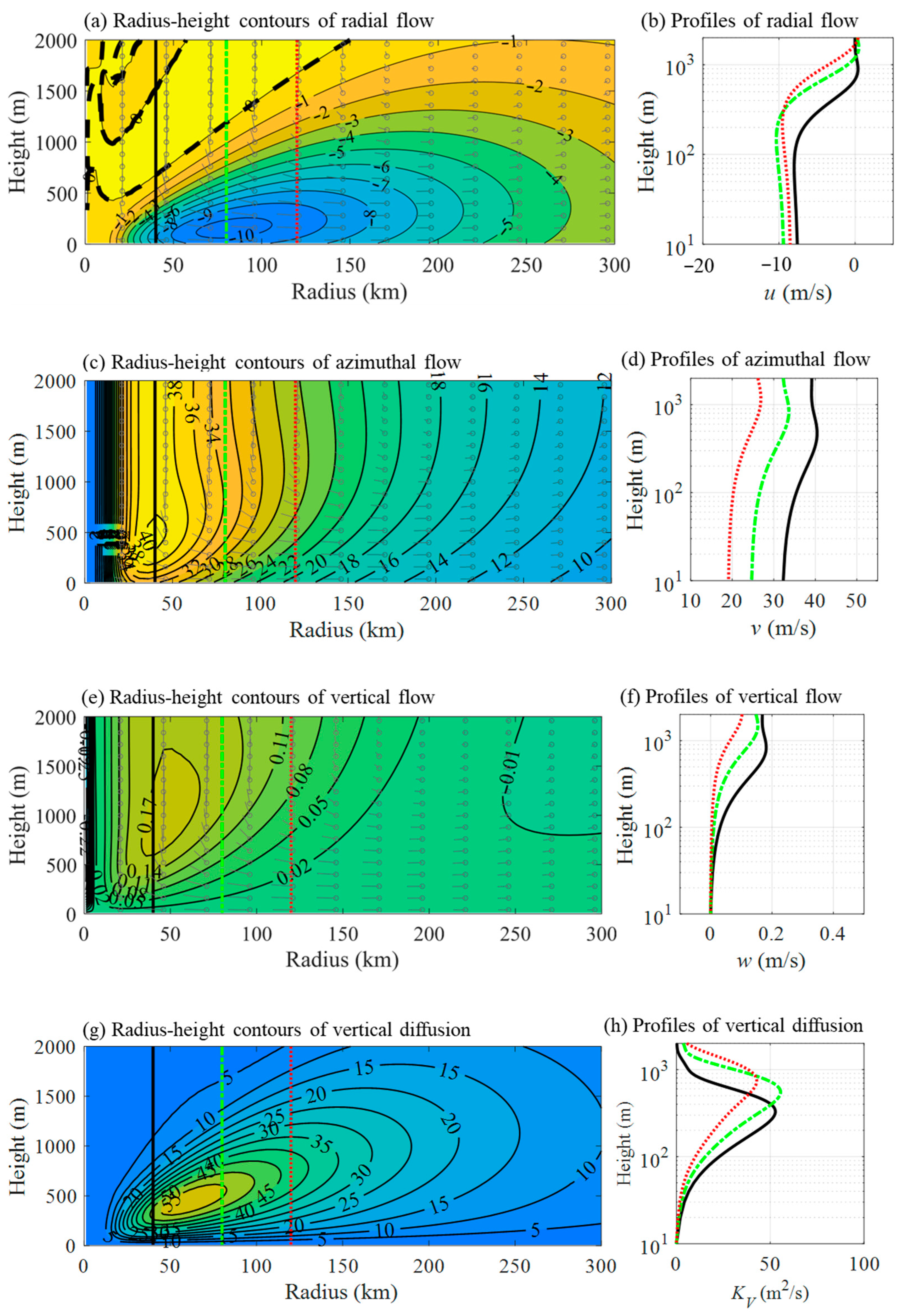
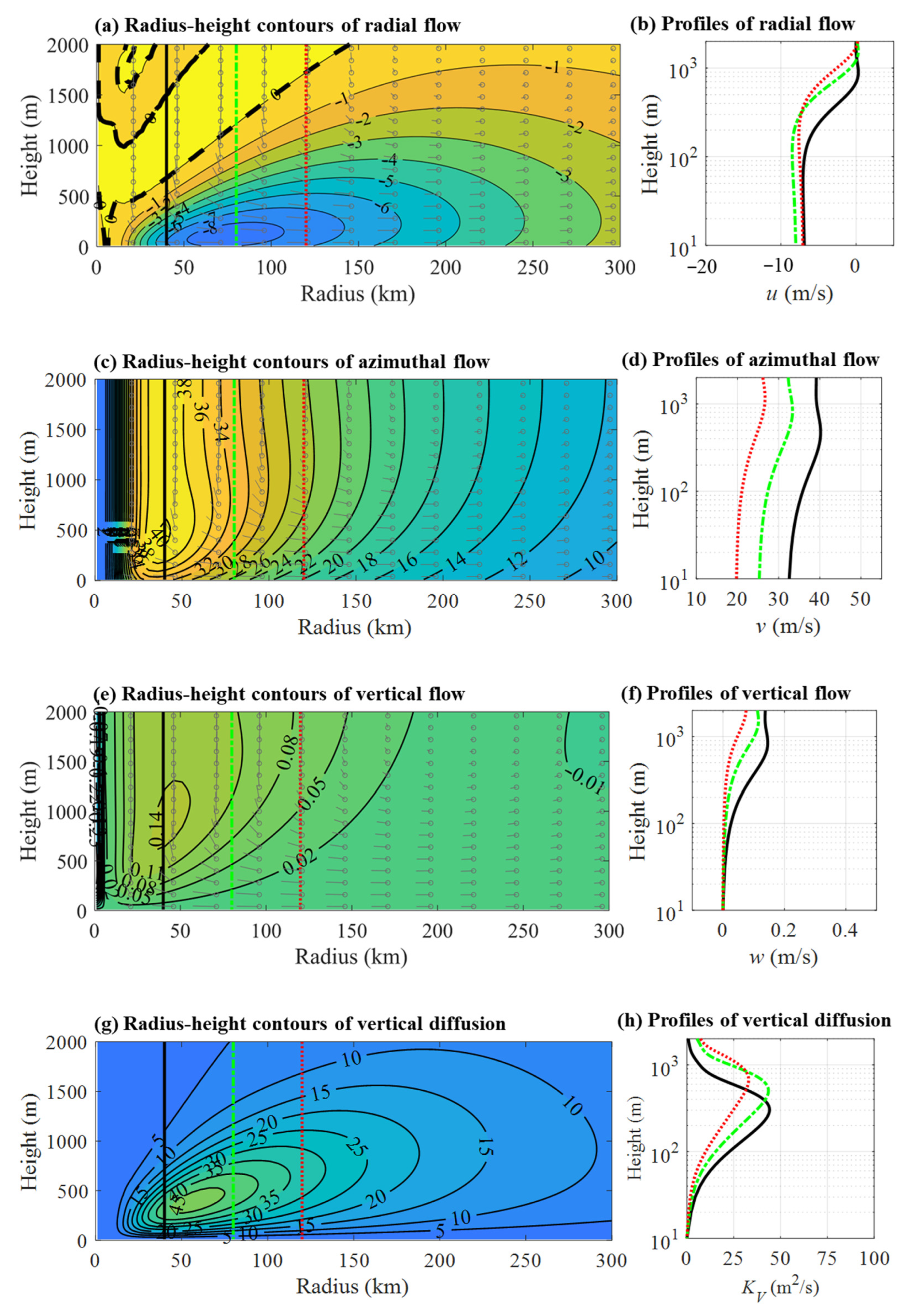
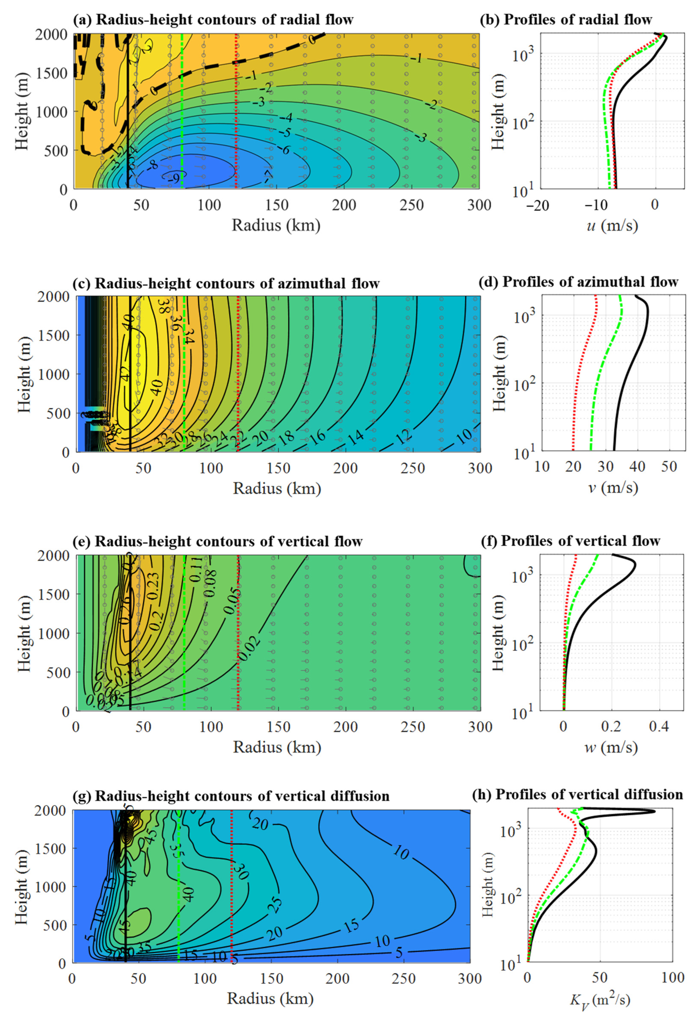
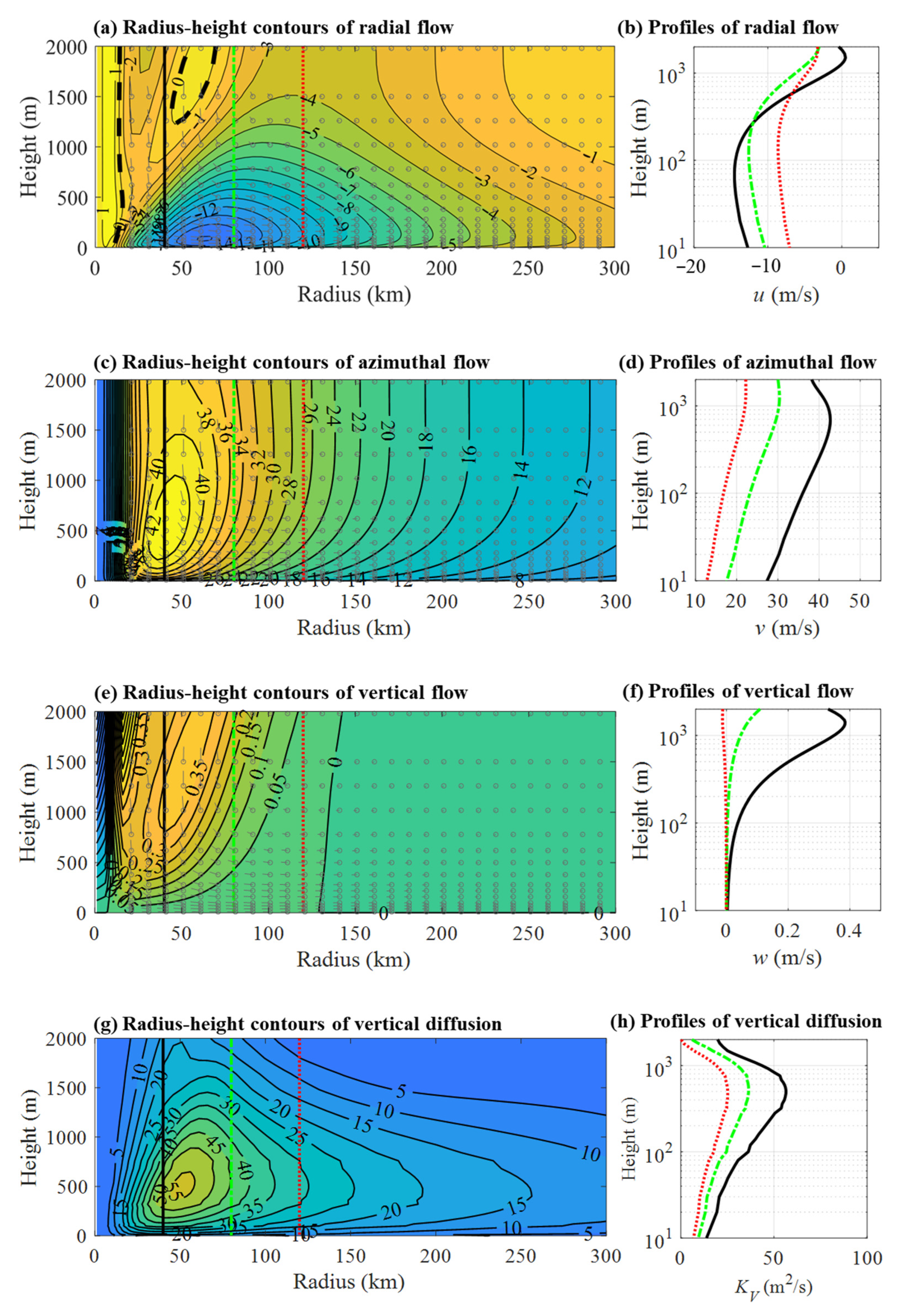
In this section, a series of simulations are conducted using the models of M95, K01, Y21a, and Y21b to investigate the role of linear radial advection, nonlinear vertical advection, and turbulent diffusion in shaping TC wind field structures. For all models, the upper boundary condition is specified using the parametric profile of Holland [14], with a maximum gradient wind of 40 m/s at the R_max of 40 km and a B parameter of 1.3. The TC vortex is prescribed to move toward north at 5 m/s. The corresponding gradient wind field is illustrated in Figure 1. The azimuthally averaged radius-height cross-sections of the radial, azimuthal, and vertical winds, together with the calculated vertical eddy viscosity coefficient (K_V) for these four models are investigated in Figure 5, Figure 6, Figure 7 and Figure 8, respectively.

Figure 5. Simulated azimuthally averaged flow using the model of M96. The left panel shows the radius-height contour plots of (a) radial wind, (c) azimuthal wind, (e) vertical wind, and (g) vertical diffusion coefficient, while the right panel shows the corresponding vertical profiles at R_max (black solid line), 2·R_max (green dash-dotted line), 3·R_max (red dashed line). In (a), the black bold dashed lines denote the outflow region. In the contour plots of left panel, the black solid, green dash-dotted, and red dashed lines indicate the location of R_max, 2·R_max, and 3·R_max, respectively. gray arrows in (a,c,e) denote wind directions.

Figure 6. Simulated azimuthally averaged flow using the model of K01. The left panel shows the radius-height contour plots of (a) radial wind, (c) azimuthal wind, (e) vertical wind, and (g) vertical diffusion coefficient, while the right panel shows the corresponding vertical profiles at R_max (black solid line), 2·R_max (green dash-dotted line), 3·R_max (red dashed line). In (a), the black bold dashed lines denote the outflow region. In the contour plots of left panel, the black solid, green dash-dotted, and red dashed lines indicate the location of R_max, 2·R_max, and 3·R_max, respectively. gray arrows in (a,c,e) denote wind directions.

Figure 7. Simulated azimuthally averaged flow using the model of Y21a. The left panel shows the radius-height contour plots of (a) radial wind, (c) azimuthal wind, (e) vertical wind, and (g) vertical diffusion coefficient, while the right panel shows the corresponding vertical profiles at R_max (black solid line), 2·R_max (green dash-dotted line), 3·R_max (red dashed line). In (a), the black bold dashed lines denote the outflow region. In the contour plots of left panel, the black solid, green dash-dotted, and red dashed lines indicate the location of R_max, 2·R_max, and 3·R_max, respectively. gray arrows in (a,c,e) denote wind directions.

Figure 8. Simulated azimuthally averaged flow using the model of Y21b, and K_V is calculated using Equation (18). The left panel shows the radius-height contour plots of (a) radial wind, (c) azimuthal wind, (e) vertical wind, and (g) vertical diffusion coefficient, while the right panel shows the corresponding vertical profiles at R_max (black solid line), 2·R_max (green dash-dotted line), 3·R_max (red dashed line). In (a), the black bold dashed lines denote the outflow region. In the contour plots of left panel, the black solid, green dash-dotted, and red dashed lines indicate the location of R_max, 2·R_max, and 3·R_max, respectively. gray arrows in (a,c,e) denote wind directions.

It should be noted that K_V is prescribed as a constant value of 50 m²/s in the models of M95, K01, and Y21a, whereas in Y21b, it is diagnosed dynamically from the simulated wind components of u and v as,

$$K_V={\left[{\displaystyle \frac{1}{{\left(\kappa \cdot z\right)}^{-1}+l_{\infty }^{-1}}}\right]}^2\cdot \sqrt{{\left({\displaystyle \frac{\mathsf{\partial }u}{\mathsf{\partial }z}}\right)}^2+{\left({\displaystyle \frac{\mathsf{\partial }v}{\mathsf{\partial }z}}\right)}^2},$$

(18)

where l_∞ is the asymptotic mixing length, set as 80 m following the study of Kepert [21]. For model comparisons carried in this section, K_V values shown in Figure 5, Figure 6 and Figure 7 are re-calculated using Equation (18).

3.1.1. Simulation Results of M95

According to the simulation results of M95, Figure 5a shows that the inflow layer depth increases outward, increasing from about 0.5 km at a radius of 25 km (with in the TC eyewall) to about 2 km at 150 km. The maximum inflow and outflow wind speeds are about 10.35 m/s and 0.47 m/s, respectively. As indicated in Figure 5c, the azimuthal flow exhibits a pronounced super-gradient structure within the radius of 3·R_max and the super-gradient flow primarily occurs in the upper portion of the inflow layer and the lower portion of the outflow layer, as in the simulations studies carried out by Kepert [21]. The peak azimuthal wind speed reaches 40.42 m/s located near the R_max in the upper inflow region. The maximum vertical updraft wind speed (0.18 m/s) occurs just outside R_max, while weak subsidence develops beyond approximately 250 km, as shown in Figure 5e. The calculated K_V shown in Figure 5g reaches its maximum near the height of 500 m between R_max and 2·R_max with a peak value of 59 m²/s. The spatial distribution of K_V occurs upward, which aligns with the primary inflow region, indicating enhanced turbulent mixing in this zone.

For the vertical profiles shown in the right panel of Figure 5, the vertical structure of azimuthal wind (Figure 5d) indicates that the near-surface wind speed does not follow a logarithmic profile but instead increases nearly linear within the height lower than 100 m. Observations of Powell, et al. [42] demonstrate that the logarithmic wind profile should typically extend to a height of at least 300 m (see their Figure 1). This deficiency arises from the assumption of a constant K_V value of 50 m²/s, which results in a linear rather than logarithmic dependence of wind speed on height near the surface. Considering that diagnosing K_V directly is challenging or computational-heavy in analytical TC wind field models, modifications to K_V, such as those proposed by Fang, et al. [49], which approximate K_V based on TC parameters and locations parameters (such as ∆p and z₀), can help to mitigate this discrepancy.

3.1.2. Simulation Results of K01

Simulation results from the model of K01 are presented in Figure 6. Recall that the primary difference between K01 and M95 lies in the inclusion of linear tangential advection terms (v_g/r∙∂u′/∂λ and v_g/r∙∂v′/∂λ). The inflow layer depth in K01 is generally comparable to that in M95. However, both the maximum inflow and outflow wind speeds are noticeably weaker in K01, with values of 8.53 m/s and 0.32 m/s, respectively, representing reductions of 17.6% and 32% relative to M95. The azimuthal flow near the top of the inflow layer is also less strongly super-gradient, with a maximum azimuthal wind speed of 40.18 m/s. The peak upward velocity reaches 0.145 m/s, which is 19.4% weaker than that in M95, and occurs slightly outside the R_max. The radius at which the vertical velocity transitions from upward to downward motion increases to approximately 280 km. The spatial distribution of K_V remains generally similar to that in M95, but its magnitude is smaller, with a maximum value of only 47.6 m²/s. The differences between the two models arise from the effects of tangential advection in K01, which smooths the azimuthal variations in u and v. Specifically, the tangential advection weakens the inflow velocity, thereby leading to a reduction in K_V.

The vertical profiles in Figure 6b show that the inflow wind speed at R_max remains nearly constant with height below 100 m and gradually turns to outflow above approximately 600 m. The azimuthal flow in Figure 6d increases almost linearly with height, again deviating from the expected logarithmic profile. The height of super-gradient flow increases progressively from about 400 m at R_max to approximately 900 m at 3·R_max. These features are generally consistent with those observed in M95. Overall, the inclusion of tangential advection weakens the radial inflow, vertical motion, and K_V, while exerting only minor influence on the azimuthal flow, partly owing to its much larger magnitude relative to the radial velocity components u.

3.1.3. Simulation Results of Y21a

Figure 7 presents the simulation results from the model of Y21a, in which the nonlinear vertical advection terms of w∙∂u/∂z and w∙∂v/∂z are additionally considered compared to K01 and M95. As shown in Figure 7a, the inflow layer depth is approximately 500 m within the TC eyewall, increases rapidly around R_max to about 1200 m, and gradually deepens to 2 km at a radius of 200 km. Compared with Figure 6a, the increase in inflow layer depth at R_max is associated with strong upward motion occurring the TC eyewall (Figure 7e). As indicated in Figure 7a,c, both the radial and azimuthal wind speeds are generally stronger than those simulated in K01. The maximum inflow and outflow wind speeds are 9.07 m/s and 2.15 m/s, respectively, while the maximum azimuthal wind speed is 43.13 m/s, occurring at a height of approximately 1000 m. The peak vertical upward velocity is about 0.30 m/s, roughly twice that of K01. These simulation results agree well with the findings of Kepert [4], who noted that analytical models (such as M95 and K01) remove several non-negligible terms (such as the vertical advection term), leading to underestimation of outflow strength and super-gradient flow. Incorporating tangential and vertical advection terms, as in Y21a, helps to mitigate these deficiencies and produces a more realistic wind field structure.

Moreover, in Figure 7g, the distribution of K_V within the inflow region is much similar to that in K01. However, K_V exhibits irregularly in the region of outflow, with much larger values occuring near R_max at a height of 1900 m. Further examination indicates that this behavior is induced by the simulated radial flow, which becomes increasingly inhomogeneous above approximately 3 km. Nevertheless, the model of Y21a demonstrates superior performance compared to linear models of K01 and M95 in simulating the TC boundary wind field.

3.1.4. Simulation Results of Y21b

The numerical simulation results of Y21b are presented in Figure 8. As shown in Figure 8a, the inflow layer produced by Y21b is significantly deeper than that simulated by Y21a, with a maximum inflow velocity of approximately 15.1 m/s, being 66.5% larger than that in Y21a. The vertical profiles of radial wind Figure 8b exhibit a similar structure to those reported by Kepert [21] (their Figure 5b), featuring a moderate increase in inflow magnitude with height in the lowest few hundred meters, followed by a gradual reversal to outflow. This behavior reflects the typical secondary circulation pattern driven by surface friction and the associated angular momentum transport in TC boundary layers.

The maximum azimuthal wind speed in Y21b reaches 43.7 m/s, which is comparable to 43.13 m/s obtained in Y21a. As shown in Figure 8d, the azimuthal wind exhibits a logarithmic profile up to several hundred meters, consistent with the field observations of Powell, et al. [42] and confirming the ability of Y21b to reproduce near-surface wind characteristics observed in real TCs. Strong upward motion is concentrated near the eyewall (Figure 8e) and tilts outward above approximately 1000 m, while weak subsidence dominates the outer regions (r > 130 km). Additionally, a strong downward trend is evident near the TC center (r = 0), aligning with the established understanding that a pronounced downward motion exists within the eye of a TC. The distribution of K_V in Figure 8g exhibits a pattern similar to that in Y21a but with substantially higher peak values, up to 56.44 m²/s, indicating enhanced turbulent mixing and vertical momentum exchange in Y21b’s boundary layer parameterization.

3.1.5. Comparison of Radial Profiles

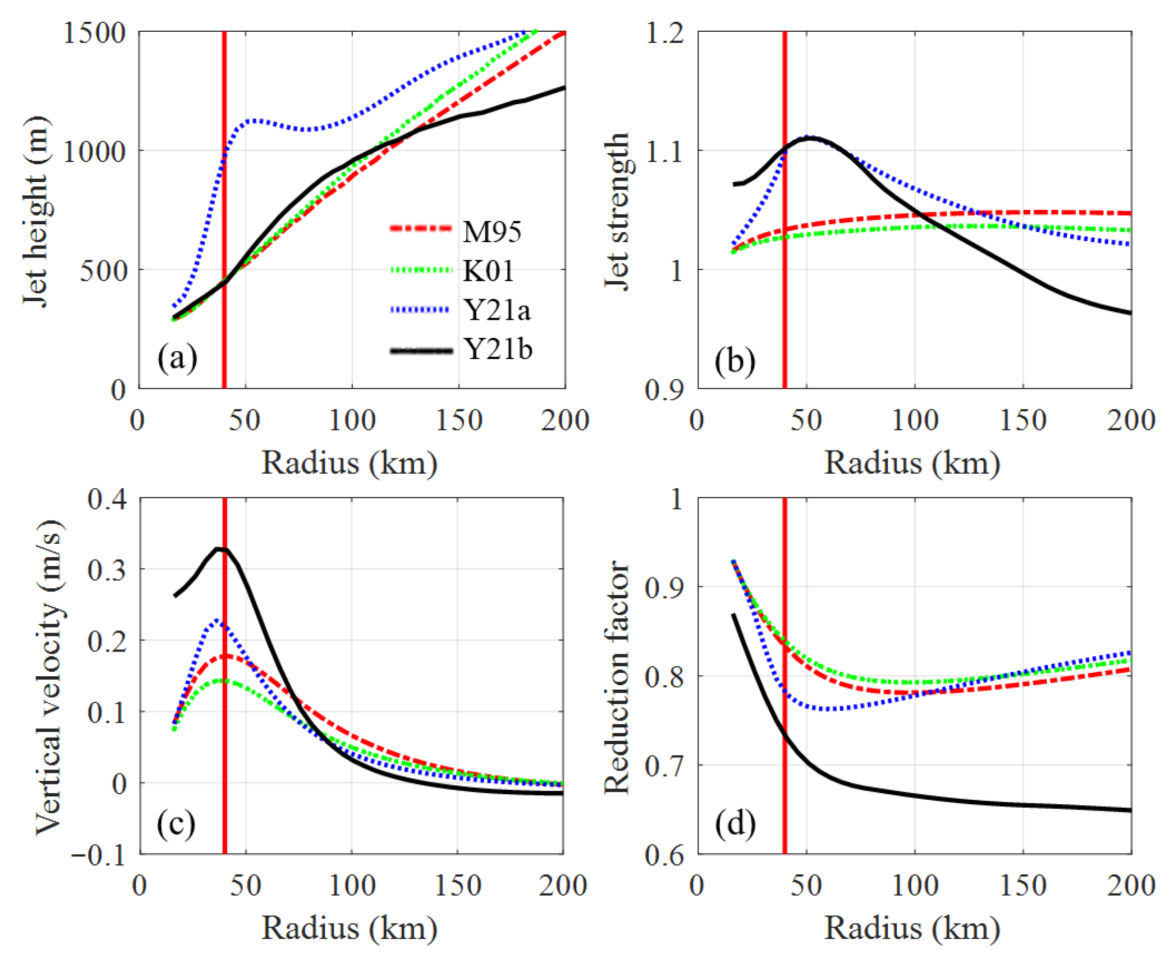
Further analysis is conducted on the simulated radial profiles of jet height, jet strength, vertical velocity, and surface wind reduction factor, as shown in Figure 9. The jet height (Figure 9a) is defined as the height of maximum wind speed in radius-height field, while the jet strength (Figure 9b) is quantified as the ratio of maximum wind speed to the gradient wind speed. The surface wind reduction factor (Figure 9d) is defined as the ratio of the gradient wind speed to the corresponding 10 m surface wind speed.

Figure 9. Comparisons of (a) jet height, (b) jet strength, (c) vertical velocity at the height of 1000 m, and (d) surface wind reduction factor among the models of M95 (red dash-dotted line), K01 (green dashed line), Y21a (blue dotted line), and Y21b (black solid line). The jet height is defined as the height of maximum wind speed, while the jet strength is the ratio of maximum wind speed to the gradient wind speed. The wind reduction factor is defined as the ratio of gradient wind speed to the 10 m surface wind speed. The vertical red lines in each panel indicate the R_max.

In the models of M95 and K01, the jet height increases nearly linearly with radius, from about 300 m within the TC eyewall to about 1500 m in a radius of 200 km. In contrast, the jet height in Y21a is much higher, as the consideration of vertical advection terms shifts the location of the maximum azimuthal wind upward. When the full TC dynamic processes are incorporated in Y21b, the jet height becomes slightly higher around 2·R_max but lower beyond a radius of 150 km compared with M95 and K01. In Y21a, the inclusion of vertical advection enhances the upward transport of tangential momentum from lower levels of the boundary layer toward the upper inflow layer, amplifying the super-gradient flow aloft. However, the horizontal diffusion is neglected, which in reality redistributes momentum laterally and partially limits vertical acceleration. The combination of enhanced upward transport and unconstrained vertical acceleration produces the substantially greater vertical jet height observed in Y21a. This is the reason why the model of Y21a produces a more pronounced vertical structure compared to other models, despite having a similar maximum tangential wind near the surface.

As shown in Figure 9b, the maximum jet strength in Y21a and Y21b reaches approximately 1.11, while it is much weaker in M95 and K01 due to the simplification of dynamic equations. The vertical velocity profiles (Figure 9c) increase with radius within the TC eyewall and gradually decrease in outer regions. Among the models, Y21b exhibits the strongest upward motion near R_max, followed by Y21a, M95, and K01.

The surface wind reduction factor in Figure 9d displays a nonlinear variation with radius. The factor is approximately 0.9 at a radius of 10 km, decreasing to about 0.8 in M95, K01, and Y21a at radius of 200 km, and 0.65 in Y21b. These results are constant with the values summarized in Table 1. Such behavior suggests that the assumption of a constant reduction factor, as commonly adopted in previous analytical studies, may lead to significant errors in estimating near-surface wind speeds under varying TC structures and dynamic conditions.

3.1.6. Comparison of Model Computational Efficiencies

Based on the idealized TC case investigated in this section, the computational efficiencies of the four models are compared in Table 3. All simulations are performed on a desktop computer equipped with an Intel Core i9-14900 KF processor and 64.0 GB of RAM. Owing to its analytical formulation, K01 is the most computationally efficient model, requiring only 0.8 s to simulate a TC snapshot. The model of M95 ranks next, with a computation time of 6.9 s. This is because iterative procedures are needed to calculate the frictionally induced wind components. After incorporating the vertical advection process and employing iteration solutions for boundary layer wind fields, Y21a requires approximately three times the computation time of M95. In contrast, Y21b is the most time-consuming, taking 212 s due to its fully nonlinear numerical structure, which significantly increases computational complexity.

Table 3. Computational time required by the models of M95, K01, Y21a, and Y21b for simulating a single TC snapshot.

	M95	K01	Y21a	Y21b
Time (s)	6.9	0.8	24.22	212

3.2. Comparisons with WRF Results: Typhoon Mangkhut (2018)

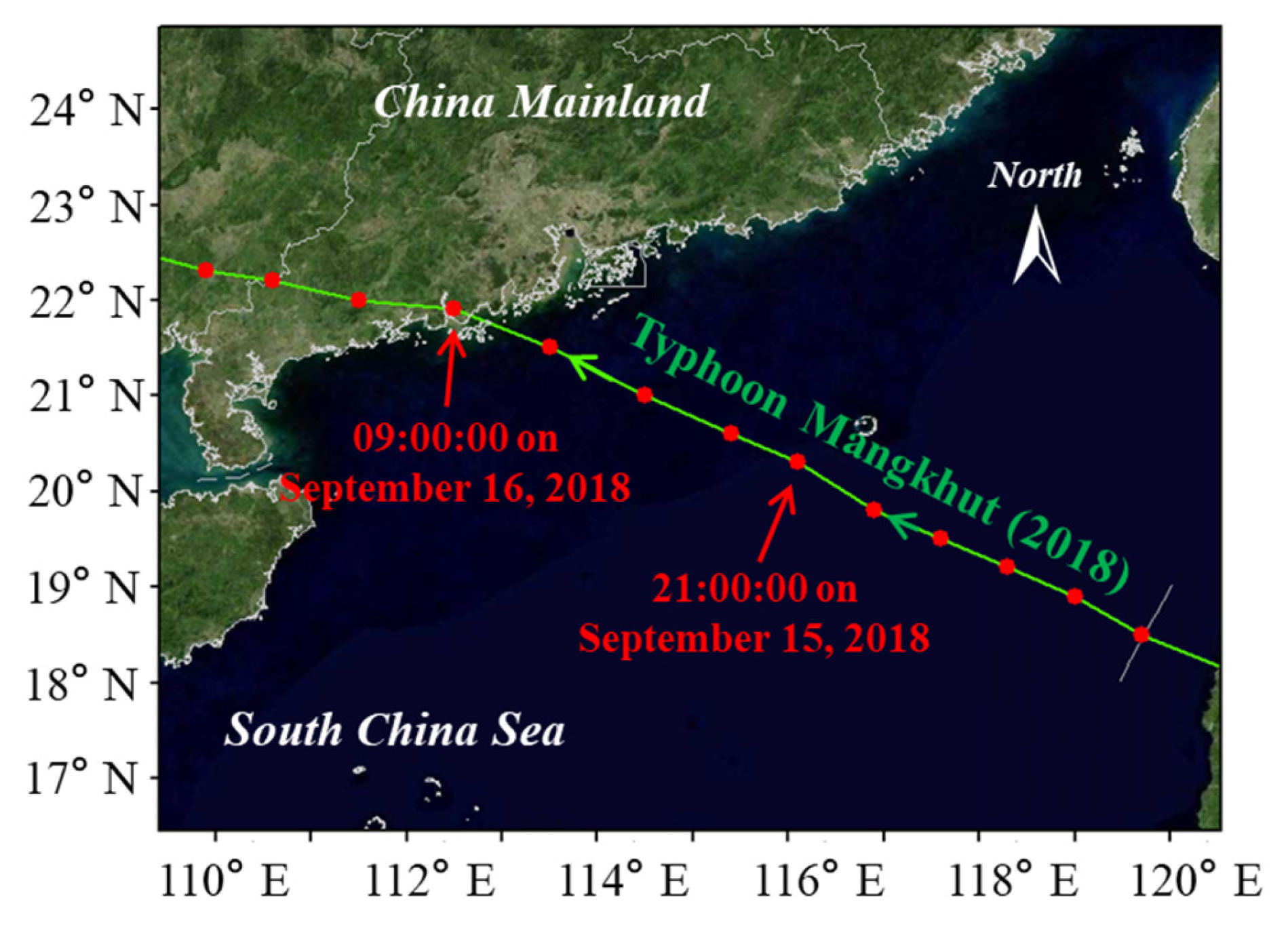
The Weather Research and Forecasting (WRF) model [53] is a mesoscale numerical weather prediction system widely used for both atmospheric research and operational forecasting. It is capable of reproducing TC wind fields under realistic atmospheric conditions and it has been widely applied to investigate TC structure and evolution [54,55,56]. To evaluate model performance in simulating real TC wind fields, Super Typhoon Mangkhut (2018) is selected as a case study, with WRF simulation results treated as reference “ground truth” for comparison. Typhoon Mangkhut originated on 5 September 2018, over the North Pacific Ocean. It was one of the most destructive TCs to make landfall in Guangdong Provance, China. Figure 10 shows the track of Typhoon Mangkhut. At 21:00:00 on 15 September 2018, the TC was over the South China Sea, and by 09:00:00 on 16 September 2018, it made landfall, with part of its wind field over the ocean and the remainder over land. The TC wind fields at these two specific time points are studied in this section.

Figure 10. The track of Super Typhoon Mangkhut (2018). Green arrows are the TC moving direction. Red dots are the locations of TC center.

The WRF-ARW dynamical core (version 4.0) is utilized to simulate the Super Typhoon Mangkhut (2018) using a three-nested domain configuration with horizontal grid spacings of 45 km, 15 km, and 5 km. The physical parameterization schemes include the Yonsei University (YSU) planetary boundary layer scheme, the Noah land surface model, the Dudhia shortwave radiation scheme, the Rapid Radiative Transfer Model (RRTM) longwave radiation scheme, the Monin–Obukhov surface layer scheme, and the WRF Single-Moment 6-class (WSM6) microphysics scheme. The initial and boundary conditions are derived from the NCEP Final (FNL) Analysis data [57] with a spatial resolution of 1° × 1° and a temporal resolution of 6 h. The WRF model simulation is initialized 24 h prior to the selected event, and model outputs are saved at 3 h intervals.

It should be noted that the WRF simulations inherently contain errors and biases compared to real conditions. In this section, the results of WRF are treated as a physically based reference to evaluate how well the parametric models are in reproducing the boundary layer structures.

3.2.1. TC Wind Field over the Ocean

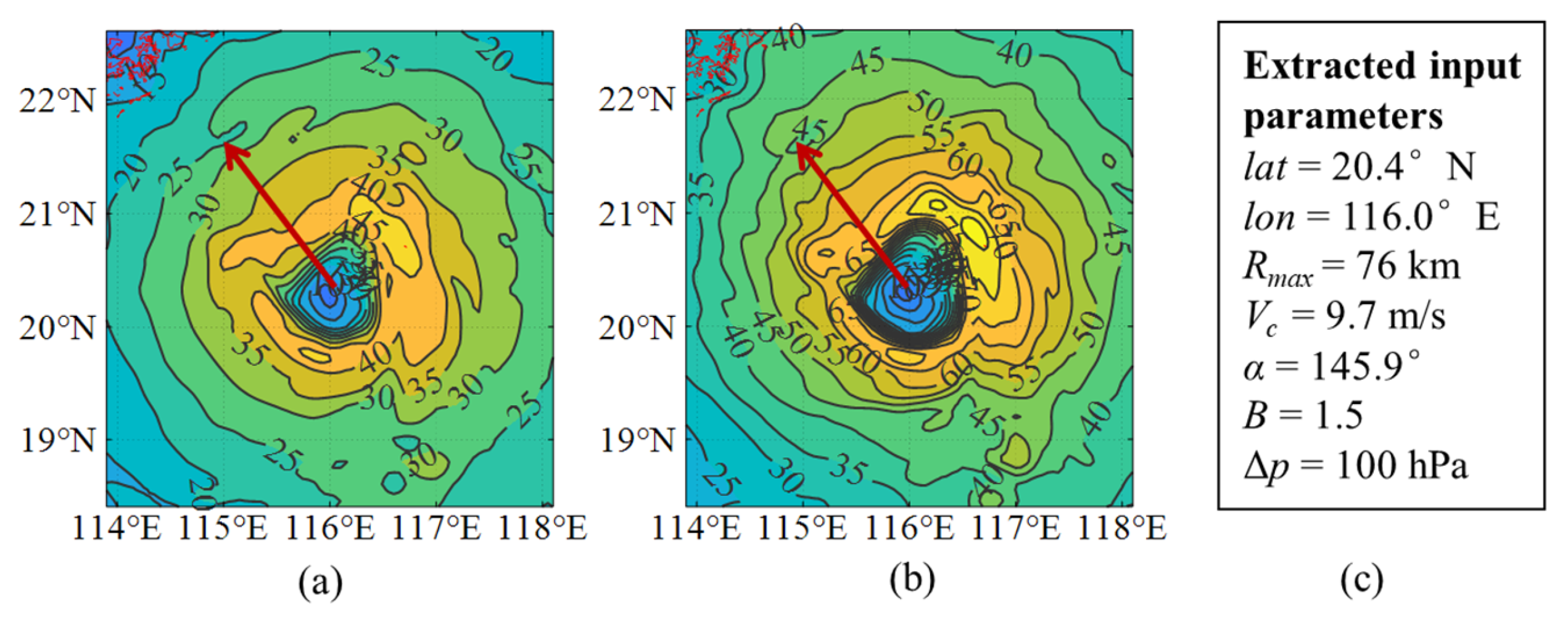
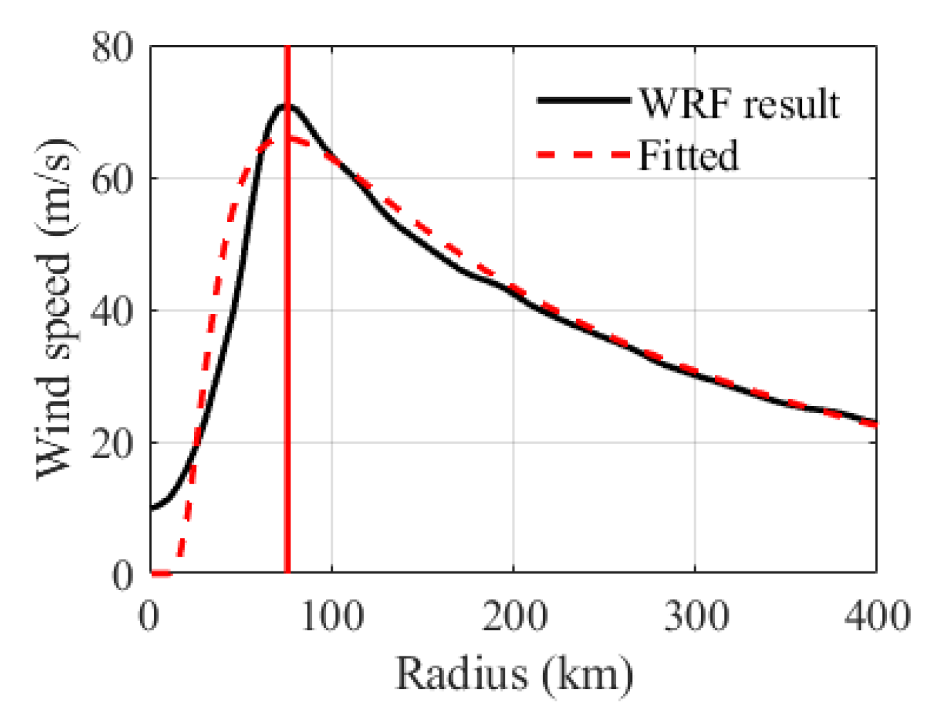
The horizontal wind fields simulated by WRF at heights of 10 m and 1000 m are shown in Figure 11. At the time of 21:00:00 on 15 September 2018, Typhoon Mangkhut was moving over the ocean, with its center located at (20.4° N, 116.0° E), R_max of 76 km, moving velocity of 9.7 m/s, and moving direction of 145.9°, as shown in Figure 11c. Considering that the gradient wind field serves as the upper boundary condition for the models of M95, K01, Y21a, and Y21b, the parameters of B and ∆p are obtained through fitting the azimuthally averaged radial wind profile of WRF using Equation (1). In this study, the WRF wind field at 1000 m is treated as the gradient wind field. The radial wind profiles of WRF and the fitted result are shown in Figure 12. It can be found that the fitted profile closely reproduces the trends and magnitudes of the WRF results, providing a consistent basis for subsequent wind field comparisons.

Figure 11. WRF simulated horizontal wind fields of Typhoon Mangkhut (2018) at 21:00:00 on 15 September 2018, over the ocean. (a) Wind field at the height of 10 m; (b) wind field at the height of 1000 m; (c) input parameters for the parametric TC wind field models extracted from the 1000 m wind field. The red arrow indicates the TC moving direction.

Figure 12. Gradient wind profile (black solid line) derived from the WRF-simulated 1000 m wind field shown in Figure 11b, along with the fitted results (red dashed line) using Equation (1) based on the parameters shown in Figure 11c. The vertical red line indicates the R_max.

For Typhoon Mangkhut moving over the ocean, the simulated wind fields at heights of 10 m and 1000 m, using the parameters shown in Figure 11c, are presented in Figure 13 and Figure 14, respectively. At the surface (Figure 13), the wind fields of K01, Y21a, and Y21b are broadly similar, with maximum wind speed of about 56.8 m/s, located to the right of the TC’s moving direction. The simulation of M95 exhibits a slightly smaller maximum value of 54.8 m/s. At the height of 1000 m (Figure 14), Y21a produces the highest maximum wind speeds of 95.2 m/s, which is larger than the values obtained in K01 and Y21b (about 84.6 m/s), and M95 (about 71 m/s). Different from the other three models, the maximum wind of Y21a occurs near the front of the TC’s moving direction, showing a counterclockwise rotation from the surface to the upper levels.

Figure 13. Simulated 10 m wind fields of Typhoon Mangkhut at 21:00:00 on 15 September 2018, over the ocean, by the models of (a) M95, (b) K01, (c) Y21a, and (d) Y21b, using the input parameters shown in Figure 11c.

Figure 14. As is in Figure 13, but for the simulated wind fields at the height of 1000 m.

Quantitative comparisons of the wind fields are carried out in Figure 15 and Figure 16. As can be found in Figure 15, the surface wind speeds simulated by M95, K01, and Y21a are generally higher than those in WRF results, exceeding them by about 20%. In contrast, the surface wind speeds simulated by Y21b are in good agreement with WRF, closely following the 45° line. The Pearson correlation coefficient (R) for all four models is similar, about 0.91. At the height of 1000 m (Figure 16), the simulated wind fields show little bias among the four models, with the data points nearly evenly distributed along the line of 45°. The R values for M95, K01, Y21a, and Y21b are 0.91, 0.90, 0.86, and 0.92, respectively, indicating relatively good performances for all models. Overall, while all four TC wind field models perform similarly for the TC moving over the ocean, Y21b demonstrates the most accurate representation of surface wind fields.

Figure 15. Comparisons of the simulated TC wind fields (as is in Figure 13, at the height of 10 m) by the models of (a) M95, (b) K01, (c) Y21a, and (d) Y21b with the results of WRF. R in each panel indicates the Pearson correlation coefficient.

Figure 16. Comparisons of the simulated TC wind fields (as is in Figure 14, at the height of 1000 m) by the models of (a) M95, (b) K01, (c) Y21a, and (d) Y21b with the results of WRF. R in each panel indicates the Pearson correlation coefficient.

3.2.2. TC Wind Field at Landfall

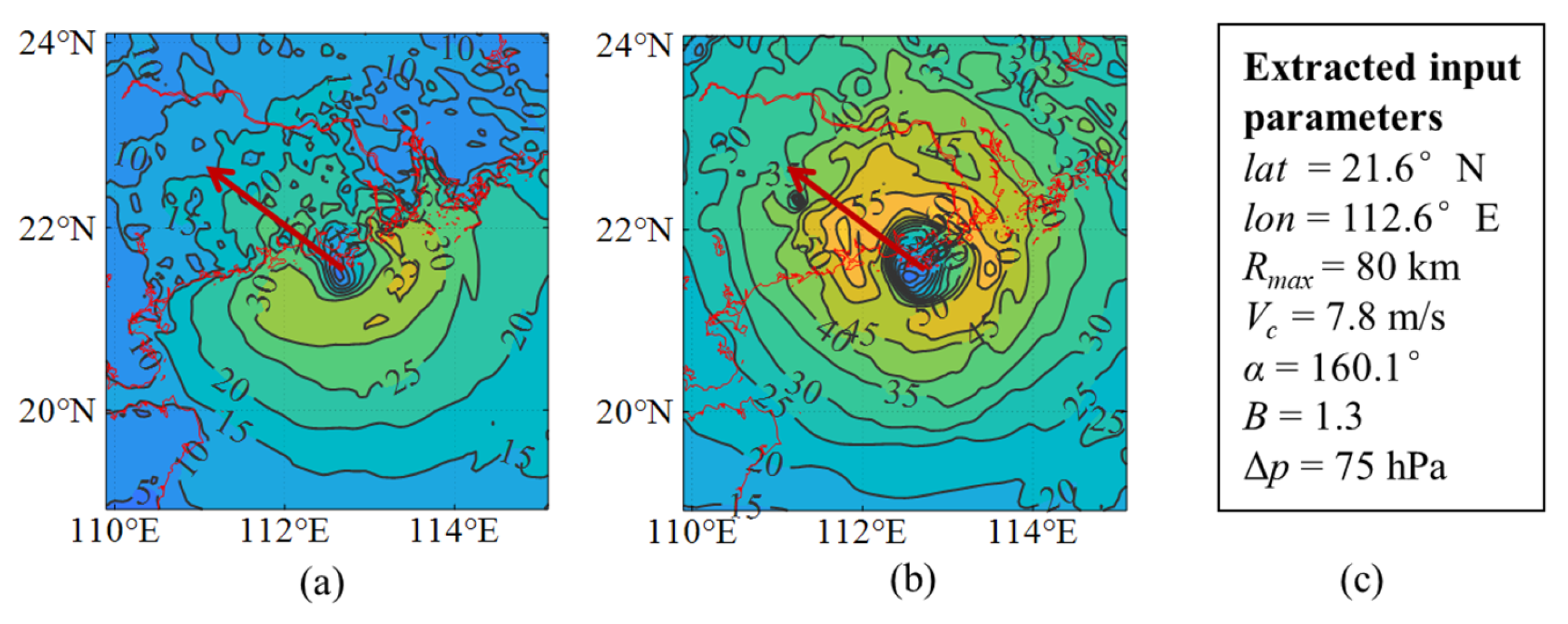
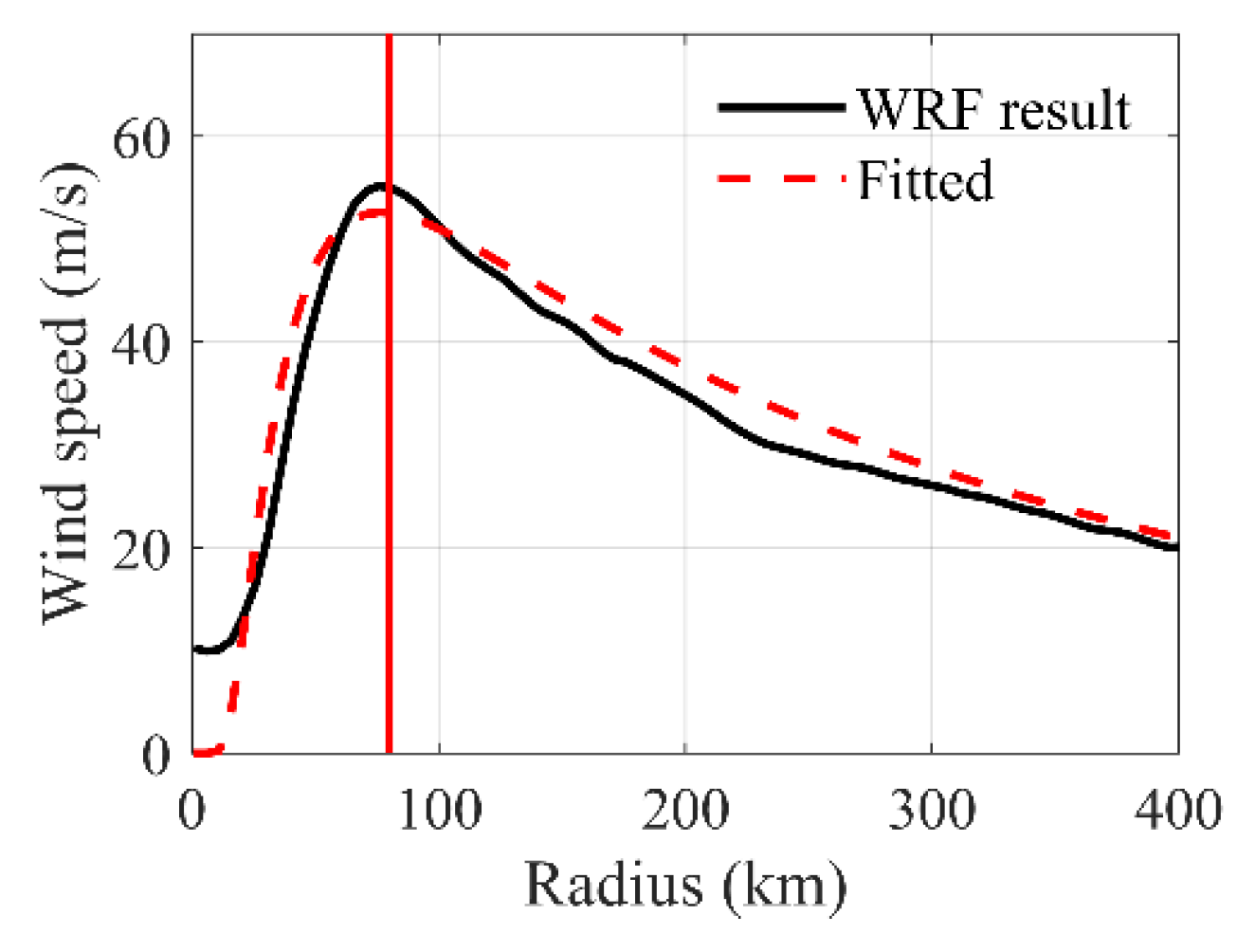
Figure 17 shows the horizontal wind fields simulated by WRF during Typhoon Mangkhut’s landfall at 09:00:00 on 16 September 2018. As presented in Figure 17a, the surface wind field indicates that wind speeds over the ocean are much higher than those over land. This difference arises from the inhomogeneous land cover and complex topographic, which act as obstacles to near-surface winds and suppress wind speed development. With increasing height, the effects of land cover and topographic diminish, and the wind field at 1000 m (Figure 17b) retains the characteristic vortex structure, with a clearly identifiable eyewall. The maximum wind speed in Figure 17b occurs on the right-hand side of the TC’s moving direction. Input parameters used for TC wind field simulations are summarized in Figure 17c. The TC center is located at (21.6° N, 112.6° E), with the R_max of 80 km, the moving velocity of 7.8 m/s, the moving direction of 160.1°, and the B parameter of 1.3. The radial wind profiles obtained from the WRF simulation and the fitted curve based on Equation (1) using above parameters are compared in Figure 18.

Figure 17. WRF-simulated horizontal wind fields of Typhoon Mangkhut (2018) at 09:00:00 on 16 September 2018, during landfall. (a) Wind field at the height of 10 m; (b) wind field at the height of 1000 m; (c) input parameters for the parametric TC wind field models extracted from the 1000 m wind field. The red arrow indicates the TC moving direction.

Figure 18. Gradient wind profile (black solid line) derived from the WRF simulated 1000 m wind field shown in Figure 17b, along with the fitted results (red dashed line) using Equation (1) based on the parameters shown in Figure 17c. The vertical red line indicates the R_max.

The wind fields shown in Figure 19 and Figure 20 are simulated by the models of M95, K01, Y21a, and Y21b, using the parameters summarized in Figure 17c. As described by Yang, et al. [20], the model of Y21b is designed to incorporate the effects of various land cover and topography through adopting a terrain-following coordinate system proposed by Tzvi and Somerville [23]. The spatial patterns of the simulated surface wind field by Y21b (Figure 19d) are consistent with those produced by WRF (Figure 17a). The maximum wind speed reaches about 40 m/s and is located over the ocean. Over land, the wind field appears relatively irregular, which is similar to the WRF results. In contrast, the original versions of M95, K01, and Y21a cannot consider the spatially varying effects of land–sea transitions, as they simplify the complex turbulent exchange by adopting a constant drag coefficient. Consequently, the wind fields simulated by these three models show notable discrepancies from the WRF results for the TC at landfall. As shown in Figure 21, the R values for M95, K01, and Y21a are relatively low (0.71, 0.59, 0.70, respectively), while Y21b achieves the highest R value of 0.93, indicating a substantially improved agreement with the WRF simulation.

Figure 19. Simulated 10 m wind fields of Typhoon Mangkhut at 09:00:00 on 16 September 2018, during landfall, by the models of (a) M95, (b) K01, (c) Y21a, and (d) Y21b, using the input parameters shown in Figure 17c.

Figure 20. As is in Figure 19, but for the simulated wind fields at the height of 1000 m.

Figure 21. Comparisons of the simulated TC wind fields (as is in Figure 19, at height of 10 m) by the models of (a) M95, (b) K01, (c) Y21a, and (d) Y21b with the results of WRF. R in each panel indicates the Pearson correlation coefficient.

At the height of 1000 m, the influence of underlaying surface diminishes, allowing the models of M95, K01, and Y21a to produce plausible simulation results (Figure 20a–c) compared with the WRF simulation (Figure 17b). The corresponding R values are 0.93 for M95, 0.91 for K01, and 0.90 for Y21a. However, the wind speeds simulated by these models are approximately 11% higher than those of WRF, exhibiting an upward deviation from the 45° line. The wind field generated by Y21b at 1000 m (Figure 20d) also demonstrates good agreement with WRF, with an R value of 0.90 and the simulated data points distributed closely around 45° line. Overall, the effects of the underlying surface should not be neglected, particularly for landfalling TCs. The Y21b model shows superior capability in reproducing surface wind fields during TC landfall compared with M95, K01, and Y21a. Nevertheless, at upper levels where surface effects are weaker, all four models exhibit comparable performance, although M95, K01, and Y21a slightly overestimate the wind speeds relative to WRF (Figure 22).

Figure 22. Comparisons of the simulated TC wind fields (as is in Figure 20 at height of 1000 m) by the models of (a) M95, (b) K01, (c) Y21a, and (d) Y21b with the results of WRF. R in each panel indicates the Pearson correlation coefficient.

3.2.3. Evaluation of TC Wind Field Modifications

As discussed in Section 2.3.2, the spatial heterogeneity of land surfaces can be incorporated into the TC wind field model through the drag coefficient in Equation (17). Accordingly, the models of M95, K01, and Y21a are modified to account for the effects of varying land cover. The recalculated horizontal wind fields of Typhoon Mangkhut (2018) during landfall are presented in Figure 23a–c for M95, K01, and Y21a, respectively. The corresponding scatter plots comparing the simulated wind speeds with WRF results are shown in Figure 23d–f. Moreover, direct model comparisons are carried out in Figure 24.

Figure 23. Simulated horizontal wind fields at the height of 10 m by (a) M95, (b) K01, and (c) Y21a after considering the effects of land cover (proposed in Section 2.3.2). Comparisons of the simulated wind fields with WRF for (d) M95, (e) K01, and (f) Y21a. R in each panel indicates the Pearson correlation coefficient.

Figure 24. Comparisons of the modified models with Y21b. The wind fields are obtained at the height of 10 m from (a) M95, (b) K01, and (c) Y21a after considering the effects of land cover. R in each panel indicates the Pearson correlation coefficient.

After incorporating land cover effects, the simulated wind fields at 10 m from M95, K01, and Y21a exhibit relatively higher wind speeds over the ocean and reduced wind speeds over land, showing spatial patterns consistent with those in WRF. For these three models, the simulated maximum wind speed is about 45 m/s, located on the right side of TC track and over the ocean near the coastline. The R values for M95, K01, and Y21a are 0.93, 0.90, and 0.90, respectively, representing an improvement of about 37% compared with the results (Figure 21a–c) before modifications. This enhancement demonstrates that explicitly accounting for surface roughness variability improves the representation of wind–surface interactions, especially across the land–sea transition zone where abrupt changes in drag significantly influence near-surface wind structures.

Further, direct model comparisons among M95, K01, Y21a, and Y21b are presented in Figure 24. The simulated wind speeds from M95, K01, Y21a show strong consistency with those of Y21b, having R values of 0.88, 0.87, and 0.91, respectively. As illustrated in the scatter plots, discrepancies are mainly concentrated in regions with low wind speeds (<30 m/s), primarily over land. In contrast, for higher wind speeds (>30 m/s), the results from M95, K01, and Y21a are nearly identical to those of Y21b. This phenomenon is also evident in Figure 19d and Figure 23a–c, where the TC wind speeds simulated by Y21b exhibit pronounced spatial inhomogeneity over land, similar to that observed in the WRF results (Figure 17a). This superiority performance can be attributed to the incorporation of nonlinear dynamics and the advanced terrain-following coordinate system in Y21b, which together enable a more realistic simulation of land-induced asymmetries in TC wind fields.

However, the quasi-linear rather than logarithmic vertical wind profiles observed in Figure 5d, Figure 6d and Figure 7d are not fixed through adjusting the C_d. This is because the shape of vertical wind profile is primarily controlled by K_V. A height-dependent parameterization of K_V is essential to achieve a more physically consistent vertical structure. For example, Meng, et al. [58] adopted a turbulence closure model proposed by Mellor and Yamada [59], in which K_V was calculated from turbulence kinetic energy and turbulence length. Unfortunately, despite multiple efforts, the present study was unable to reproduce their work, highlighting the need for further investigation.

4. Discussion and Limitation

Comparative evaluation of the four parametric models (M95, K01, Y21a, and Y21b) demonstrates differences in their ability to produce the TC boundary layer wind structures. These differences arise primarily from the degree of physical processes included in each model, especially the representation of turbulent diffusion, vertical advection, and surface drag. The results from both the idealized and real historical TC case simulations reveal that the fidelity of the simulated wind fields improves systematically as the governing equations evolve from linearized analytical forms to fully nonlinear numerical solutions that explicitly account for vertical and horizontal advection as well as spatially varying surface roughness.

Accurate simulation of tangential wind maxima and super-gradient jet strengths closely depends on the balance among radial and vertical advection, Coriolis force, and turbulent diffusion. Simplified linear models, such as M95 and K01, cannot fully capture these nonlinear interactions, leading to biases in both the magnitude and vertical location of the maximum wind. Furthermore, the landfalling TC case highlights the critical role of surface roughness and its parameterization. As noted by Kepert [4], abrupt transitions between sea and land surfaces can induce pronounced asymmetries and enhanced turbulence, which should not be neglected in TC wind field simulations.

Despite the obtained comparison results, several limitations remain. The evaluation relies primarily on idealized or WRF-simulated wind fields rather than direct observational data, which may introduce biases relative to real world conditions. In addition, the models of this study do not explicitly account for microphysical processes (such as small-scale turbulence) due to simplifications in the governing equations. When a TC makes landfall, the enhanced surface friction over land can trigger strong low-level convergence and boundary layer moistening, which may locally intensify updrafts and modify the radial inflow structure [18]. These processes can generate a low-level positive potential vorticity band governed by thermodynamic and microphysical feedbacks, thereby affecting the vertical momentum transport and the evolution of near-surface wind maxima [60]. Given the challenges of explicitly representing microphysical processes in parametric TC models, future improvements could focus on coupling the boundary layer model with convective parameterizations or data assimilation systems to better capture the real wind field evolution. Furthermore, extending the model evaluation to a broader range of TCs with varying intensity, size, moving velocity, and landfall angles would further enhance the robustness and generality of the findings.

5. Conclusions

In this study, four representative tropical cyclone (TC) boundary layer models of M95 [30], K01 [12], Y21a [31], and Y21b [20] are comprehensively evaluated under both idealized and real historical TC case conditions. Comparison results show that the simulated TC wind fields have a consistent improvement in physical realism and predictive accuracy as model formulations evolve from linear analytical to fully nonlinear dynamic representations.

In the idealized simulation cases, all models successfully reproduced the principal dynamical features of TC boundary layers, including low-level inflow, upper-level outflow, and super-gradient jets. However, significant differences are observed in vertical structure and jet strength. The analytical models of M95 and K01, which adopt constant eddy viscosity and simplified dynamics, produced overly smooth vertical flows and underestimated jet intensities. The model of Y21a, incorporating nonlinear vertical advection, improves the vertical momentum exchange and produces stronger, more realistic jet structures. The most physically consistent results are obtained from Y21b, which resolves the full three-dimensional nonlinear dynamics and employs dynamically diagnosed turbulence scheme. The model can produce logarithmic vertical wind profiles as observed in field measurements.

Comparisons with WRF simulations of Super Typhoon Mangkhut (2018) further demonstrated that model performance strongly depends on surface boundary condition. Over the ocean, all models can simulate the spatial TC wind field structures, but the models of M95, K01, and Y21a tend to overestimate surface wind speeds due to constant drag assumptions. The model of Y21b, which includes various surface drag and terrain-following coordinates, exhibited the best agreement with WRF. During landfall, Y21b achieves superior performance (R = 0.93 at 10 m), successfully reproducing the asymmetric wind weakening caused by heterogeneous roughness and terrain. When spatially varying surface roughness was incorporated through a land-cover-based drag coefficient in the analytical models, their correlation with WRF improved markedly by about 37%, emphasizing the importance of explicit incorporating the effects of land cover.

Investigations of this study find that physical parameterizations of vertical advection, turbulent diffusion, and surface roughness are critical for reproducing realistic TC boundary layer winds. For large-scale or rapid hazard assessments, simplified analytical models are useful due to their efficiency; however, for applications requiring high spatial fidelity, such as power transmission network risk evaluation and storm surge prediction, nonlinear models like Y21b provide substantial advantages, but with higher computational cost. Future work should focus on developing hybrid parametric–numerical approaches that integrate dynamic turbulence and surface schemes within computationally efficient frameworks, enabling TC hazard modeling with both accuracy and efficiency.

References

- Rappaport, E.N. Fatalities in the United States from Atlantic Tropical Cyclones: New Data and Interpretation. Bull. Am. Meteorol. Soc. 2014, 95, 341–346. [Google Scholar] [CrossRef]
- Chen, J.; Chavas, D.R. The Transient Responses of an Axisymmetric Tropical Cyclone to Instantaneous Surface Roughening and Drying. J. Atmos. Sci. 2020, 77, 2807–2834. [Google Scholar] [CrossRef]
- Tong, B.; Hu, G.; Deng, Y.; Huang, Y.; He, Y. Deep-learning based simulation of tropical cyclone genesis in Northwest Pacific. J. Wind Eng. Ind. Aerodyn. 2025, 257, 106003. [Google Scholar] [CrossRef]
- Kepert, J.D. A Simple Model of the Tropical Cyclone Boundary Layer at Landfall. Mon. Weather Rev. 2025, 153, 589–603. [Google Scholar] [CrossRef]
- Kepert, J.D. Landfall-Induced Changes in Tropical Cyclone Veronica’s Surface Winds. Mon. Weather Rev. 2025, 153, 605–616. [Google Scholar] [CrossRef]
- Wong, M.L.M.; Chan, J.C.L. Modeling the Effects of Land–Sea Roughness Contrast on Tropical Cyclone Winds. J. Atmos. Sci. 2007, 64, 3249–3264. [Google Scholar] [CrossRef]
- Powell, M.D.; Houston, S.H. Hurricane Andrew’s landfall in South Florida. Part II: Surface wind fields and potential real-time applications. Weather Forecast. 1996, 11, 329–349. [Google Scholar] [CrossRef]
- Powell, M.D.; Dodge, P.P.; Black, M.L. The landfall of Hurricane Hugo in the Carolinas: Surface wind distribution. Weather Forecast. 1991, 6, 379–399. [Google Scholar] [CrossRef]
- Dong, M.; Ji, C.; Chen, F.; Wang, Y. Numerical Study of Boundary Layer Structure and Rainfall after Landfall of Typhoon Fitow (2013): Sensitivity to Planetary Boundary Layer Parameterization. Adv. Atmos. Sci. 2019, 36, 431–450. [Google Scholar] [CrossRef]
- Tuleya, R.E.; Kurihara, Y. A numerical simulation of the landfall of tropical cyclones. J. Atmos. Sci. 1978, 35, 242–257. [Google Scholar] [CrossRef]
- Powell, M.D. Changes in the low-level kinematic and thermodynamic structure of Hurricane Alicia (1983) at landfall. Mon. Weather Rev. 1987, 115, 75–99. [Google Scholar] [CrossRef]
- Kepert, J. The Dynamics of Boundary Layer Jets within the Tropical Cyclone Core. Part I: Linear Theory. J. Atmos. Sci. 2001, 58, 2469–2484. [Google Scholar] [CrossRef]
- Montgomery, M.T.; Smith, R.K.; Nguyen, S.V. Sensitivity of tropical-cyclone models to the surface drag coefficient. Q. J. R. Meteorol. Soc. 2010, 136, 1945–1953. [Google Scholar] [CrossRef]
- Holland, G.J. An analytic model of the wind and pressure profiles in hurricanes. Mon. Weather Rev. 1980, 108, 1212–1218. [Google Scholar] [CrossRef]
- Willoughby, H.E.; Rahn, M.E. Parametric Representation of the Primary Hurricane Vortex. Part I: Observations and Evaluation of the Holland (1980) Model. Mon. Weather Rev. 2004, 132, 3033–3048. [Google Scholar] [CrossRef]
- Hong, H.P.; Li, S.H.; Duan, Z.D. Typhoon Wind Hazard Estimation and Mapping for Coastal Region in Mainland China. Nat. Hazards Rev. 2016, 17, 04016001. [Google Scholar] [CrossRef]
- Li, S.H.; Hong, H.P. Typhoon wind hazard estimation for China using an empirical track model. Nat. Hazards 2016, 82, 1009–1029. [Google Scholar] [CrossRef]
- Li, Y.; Cheung, K.K.W.; Chan, J.C.L. Numerical study on the development of asymmetric convection and vertical wind shear during tropical cyclone landfall. Q. J. R. Meteorol. Soc. 2014, 140, 1866–1877. [Google Scholar] [CrossRef]
- Nolan, D.S.; McNoldy, B.D.; Yunge, J. Evaluation of the Surface Wind Field over Land in WRF Simulations of Hurricane Wilma (2005). Part I: Model Initialization and Simulation Validation. Mon. Weather Rev. 2021, 149, 679–695. [Google Scholar] [CrossRef]
- Yang, J.; Chen, Y.; Tang, Y.; Yan, G.; Duan, Z. A high-fidelity parametric model for tropical cyclone boundary layer wind field by considering effects of land cover and terrain. Atmos. Res. 2021, 260, 105701. [Google Scholar] [CrossRef]
- Kepert, J.D. Choosing a Boundary Layer Parameterization for Tropical Cyclone Modeling. Mon. Weather Rev. 2012, 140, 1427–1445. [Google Scholar] [CrossRef]
- Hong, X.; Hong, H.P.; Li, J. Solution and validation of a three dimensional tropical cyclone boundary layer wind field model. J. Wind Eng. Ind. Aerodyn. 2019, 193, 103973. [Google Scholar] [CrossRef]
- Tzvi, G.-C.; Somerville, R.C.J. On the use of a coordinate transformation for the solution of the Navier-Stokes equations. J. Comput. Phys. 1975, 17, 209–228. [Google Scholar] [CrossRef]
- Fei, R.; Wang, Y.Q.; Li, Y.L. Contribution of Vertical Advection to Supergradient Wind in Tropical Cyclone Boundary Layer: A Numerical Study. J. Atmos. Sci. 2021, 78, 1057–1073. [Google Scholar] [CrossRef]
- Snaiki, R.; Wu, T. An analytical model for rapid estimation of hurricane supergradient winds. J. Wind Eng. Ind. Aerodyn. 2020, 201, 104175. [Google Scholar] [CrossRef]
- Liu, J.; Li, B. A deep learning model for predicting mechanical behaviors of dynamic power cable of offshore floating wind turbine. Mar. Struct. 2025, 99, 103705. [Google Scholar] [CrossRef]
- Yang, L.; Li, B.; Dong, Y.; Hu, Z.; Zhang, K.; Li, S. Large-amplitude rotation of floating offshore wind turbines: A comprehensive review of causes, consequences, and solutions. Renew. Sustain. Energy Rev. 2025, 211, 115295. [Google Scholar] [CrossRef]
- Jian, W.; Cao, D.; Lo, E.Y.; Huang, Z.; Chen, X.; Cheng, Z.; Gu, H.; Li, B. Wave runup on a surging vertical cylinder in regular waves. Appl. Ocean Res. 2017, 63, 229–241. [Google Scholar] [CrossRef]
- Wang, X.; Qiao, D.; Jin, L.; Yan, J.; Wang, B.; Li, B.; Ou, J. Numerical investigation of wave run-up and load on heaving cylinder subjected to regular waves. Ocean Eng. 2023, 268, 113415. [Google Scholar] [CrossRef]
- Meng, Y.; Masahiro, M.; Kazuki, H. An analytical model for simulation of the wind field in a typhoon boundary layer. J. Wind Eng. Ind. Aerodyn. 1995, 56, 291–310. [Google Scholar] [CrossRef]
- Yang, J.; Chen, Y.; Zhou, H.; Duan, Z. A height-resolving tropical cyclone boundary layer model with vertical advection process. Nat. Hazards 2021, 107, 723–749. [Google Scholar] [CrossRef]
- Giammanco, I.M.; Schroeder, J.L.; Powell, M.D. GPS Dropwindsonde and WSR-88D Observations of Tropical Cyclone Vertical Wind Profiles and Their Characteristics. Weather Forecast. 2013, 28, 77–99. [Google Scholar] [CrossRef]
- Willoughby, H.E.; Darling, R.W.R.; Rahn, M.E. Parametric Representation of the Primary Hurricane Vortex. Part II: A New Family of Sectionally Continuous Profiles. Mon. Weather Rev. 2006, 134, 1102–1120. [Google Scholar] [CrossRef]
- Georgiou, P.N.; Davenport, A.G.; Vickery, B.J. Design wind speeds in regions dominated by tropical cyclones. J. Wind Eng. Ind. Aerodyn. 1983, 13, 139–152. [Google Scholar] [CrossRef]
- Batts, M.E.; ASCE, A.M.; Russell, L.R.; Simiu, E. Hurricane Wind Speeds in The United States. J. Struct. Div. 1980, 106, 2001–2016. [Google Scholar] [CrossRef]
- Du, H.; Yu, P.; Zhu, L.; Fei, K.; Gao, L. Assessing the performances of parametric wind models in predicting storm surges in the Pearl River Estuary. J. Wind Eng. Ind. Aerodyn. 2023, 232, 105265. [Google Scholar] [CrossRef]
- Chen, Y.; Duan, Z. A statistical dynamics track model of tropical cyclones for assessing typhoon wind hazard in the coast of southeast China. J. Wind Eng. Ind. Aerodyn. 2018, 172, 325–340. [Google Scholar] [CrossRef]
- Georgiou, P.N. Design Wind Speeds in Tropical Cyclone-Prone Regions; University of Western Ontario: London, ON, Canada, 1985. [Google Scholar]
- Vickery, P.J.; Skerlj, P.F.; Steckley, A.C.; Twisdale, L.A. Hurricane Wind Field Model for Use in Hurricane Simulations. J. Struct. Eng. 2000, 126, 1203–1221. [Google Scholar] [CrossRef]
- Vickery, P.J.; Skerlj, P.F.; Twisdale, L.A. Simulation of Hurricane Risk in the U.S. Using Empirical Track Model. J. Struct. Eng. 2000, 126, 1222–1237. [Google Scholar] [CrossRef]
- Sparks, P.R.; Huang, Z. Gust factors and surface-to-gradient wind-speed ratios in tropical cyclones. J. Wind Eng. Ind. Aerodyn. 2001, 89, 1047–1058. [Google Scholar] [CrossRef]
- Powell, M.D.; Vickery, P.J.; Reinhold, T.A. Reduced drag coefficient for high wind speeds in tropical cyclones. Nature 2003, 422, 279–283. [Google Scholar] [CrossRef] [PubMed]
- Powell, M.; Soukup, G.; Cocke, S.; Gulati, S.; Morisseau-Leroy, N.; Hamid, S.; Dorst, N.; Axe, L. State of Florida hurricane loss projection model: Atmospheric science component. J. Wind Eng. Ind. Aerodyn. 2005, 93, 651–674. [Google Scholar] [CrossRef]
- Vickery, P.J.; Wadhera, D.; Powell, M.D.; Chen, Y. A Hurricane Boundary Layer and Wind Field Model for Use in Engineering Applications. J. Appl. Meteorol. Climatol. 2009, 48, 381–405. [Google Scholar] [CrossRef]
- Shapiro, L.J. The Asymmetric Boundary layer Flow Under a Translating Hurricane. J. Atmos. Sci. 1983, 40, 1984–1998. [Google Scholar] [CrossRef]
- Thompson, E.F.; Cardone, V.J. Practical modeling of hurricane surface wind fields. J. Waterw. Port Coast. Ocean Eng. 1996, 122, 195–205. [Google Scholar] [CrossRef]
- Kepert, J.; Wang, Y. The Dynamics of Boundary Layer Jets within the Tropical Cyclone Core. Part II: Nonlinear Enhancement. J. Atmos. Sci. 2001, 58, 2485–2501. [Google Scholar] [CrossRef]
- Snaiki, R.; Wu, T. A linear height-resolving wind field model for tropical cyclone boundary layer. J. Wind Eng. Ind. Aerodyn. 2017, 171, 248–260. [Google Scholar] [CrossRef]
- Fang, G.; Zhao, L.; Cao, S.; Ge, Y.; Pang, W. A novel analytical model for wind field simulation under typhoon boundary layer considering multi-field correlation and height-dependency. J. Wind Eng. Ind. Aerodyn. 2018, 175, 77–89. [Google Scholar] [CrossRef]
- Holton, J.R. An Introduction to Dynamic Meteorology, 4th ed.; Elsevier Academic Press: Boston, MA, USA, 2007. [Google Scholar] [CrossRef]
- Markert, A.; Griffin, R.; Knupp, K.; Molthan, A.; Coleman, T. A Spatial Pattern Analysis of Land Surface Roughness Heterogeneity and its Relationship to the Initiation of Weak Tornadoes. Earth Interact. 2019, 23, 1–28. [Google Scholar] [CrossRef]
- Ek, M.B.; Mitchell, K.E.; Lin, Y.; Rogers, E.; Grunmann, P.; Koren, V.; Gayno, G.; Tarpley, J.D. Implementation of Noah land surface model advances in the National Centers for Environmental Prediction operational mesoscale Eta model. J. Geophys. Res. Atmos. 2003, 108, 1–12. [Google Scholar] [CrossRef]
- Skamarock, W.C.; Klemp, J.B.; Dudhia, J.; Gill, D.O.; Liu, Z.; Berner, J.; Wang, W.; Powers, J.G.; Duda, M.G.; Huang, X.Y. A Description of the Advanced Research WRF Model Version 4; NCAR/TN-556+STR; NCAR: Boulder, CO, USA, 2019. [Google Scholar]
- Xue, L.; Li, Y.; Song, L.; Chen, W.; Wang, B. A WRF-based engineering wind field model for tropical cyclones and its applications. Nat. Hazards 2017, 87, 1735–1750. [Google Scholar] [CrossRef]
- Dodla, V.B.; Desamsetti, S.; Yerramilli, A. A comparison of HWRF, ARW and NMM models in Hurricane Katrina (2005) simulation. Int. J. Environ. Res. Public Health 2011, 8, 2447–2469. [Google Scholar] [CrossRef] [PubMed]
- Wu, Y.; Wang, N.; Huang, X.; Wang, Z. Enhancing power grid resilience during tropical cyclones: Deep learning-based real-time wind forecast corrections for dynamic risk prediction. Reliab. Eng. Syst. Saf. 2025, 263, 111284. [Google Scholar] [CrossRef]
- National Centers for Environmental Prediction, N.W.S., NOAA, U.S. Department of Commerce. NCEP FNL Operational Model Global Tropospheric Analyses, Continuing from July 1999. Research Data Archive at the National Center for Atmospheric Research, Computational and Information Systems Laboratory. Boulder, CO. Available online: https://gdex.ucar.edu/datasets/d083002/ (accessed on 8 October 2024).
- Meng, Y.; Masahiro, M.; Kazuki, H. A numerical study of the wind field in a typhoon boundary layer. J. Wind Eng. Ind. Aerodyn. 1997, 67–68, 437–448. [Google Scholar] [CrossRef]
- Mellor, G.L.; Yamada, T. A Hierarchy of Turbulence Closure Models for Planetary Boundary Layers. J. Atmos. Sci. 1974, 31, 1791–1806. [Google Scholar] [CrossRef]
- Chen, Y.; Yau, M.K. Asymmetric Structures in a Simulated Landfalling Hurricane. J. Atmos. Sci. 2003, 60, 2294–2312. [Google Scholar] [CrossRef]
Disclaimer/Publisher’s Note: The statements, opinions and data contained in all publications are solely those of the individual author(s) and contributor(s) and not of MDPI and/or the editor(s). MDPI and/or the editor(s) disclaim responsibility for any injury to people or property resulting from any ideas, methods, instructions or products referred to in the content. |
© 2025 by the authors. Licensee MDPI, Basel, Switzerland. This article is an open access article distributed under the terms and conditions of the Creative Commons Attribution (CC BY) license (https://creativecommons.org/licenses/by/4.0/).