Article

A Vine Copula Framework for Non-Stationarity Detection Between Precipitation and Meteorological Factors and Possible Driving Factors

1
School of Water Conservancy and Environment, University of Jinan, Jinan 250022, China
2
Bureau of Hydrology Shandong, Jinan 250000, China
*
Author to whom correspondence should be addressed.
Atmosphere 2025, 16(11), 1262; https://doi.org/10.3390/atmos16111262
Submission received: 18 September 2025 / Revised: 19 October 2025 / Accepted: 22 October 2025 / Published: 4 November 2025
(This article belongs to the Section Meteorology)

Abstract

Increasing climate change leads to the variability of dependencies among meteorological factors. Currently, the investigation of the interdependence of meteorological variables primarily focuses on the bivariate relationships, such as precipitation and temperature or precipitation and wind speed. However, the high-dimensional dependencies among multiple meteorological factors have not been thoroughly explored. This paper proposes a statistical analysis framework that comprehensively analyzes the changes in dependencies among meteorological factors. This statistical analysis framework is based on multivariate joint distributions and enables the detection of dependency change points as well as the analysis of drivers using total probability formulations and orthogonal experiments. Taking the Huang-Huai-Hai region, a recipient area of the South-to-North Water Diversion project, as the study area, we constructed a vine copula-based multivariate joint distribution for precipitation (Pre) and six meteorological factors: temperature (Tm), maximum temperature (Tmax), minimum temperature (Tmin), wind speed (Win), relative humidity (Rhu), and the Southern Oscillation Index (SOI). The results indicate that a change point exists in the dependence of the 7-dimensional variables (Pre and six meteorological factors) in the Huang-Huai-Hai region in 2013. Tmin, Win, and Tmax are the primary driving factors affecting the precipitation–meteorological dependency relationship. The cumulative distribution function (CDF) is used to describe the probability distribution of precipitation and related meteorological factors. The optimal CDF values of the multivariate joint distribution model were achieved with Rhu and Tmax at level 3, SOI and Tm at level 2, and Win and Tmin at level 1. The results can provide a theoretical method for testing the non-stationarity of high-dimensional meteorological variable dependencies and offer conditional probability support for constructing meteorological prediction machine learning models.

1. Introduction

In recent decades, the cumulative impacts of climate change and human activities have caused significant changes in hydrometeorological factors, such as rainfall, air temperature, relative humidity, and wind speed, on regional and global scales [1]. The interrelationships between multidimensional meteorological factors are complex [2], forming intricate feedback loops between radiation, rainfall, temperature, relative humidity, and wind speed. These feedback mechanisms may lead to the occurrence of extreme weather events. However, most current studies focus directly on the dependence relationships between pairs of variables, such as P–T, P–WS, or WS–Rhu. Few studies address the identification of non-stationarity in relationships among multiple meteorological factors. This kind of smoothing analysis can help people recognize changes in the dependence relationships among multidimensional meteorological variables, including the identification of mutation points in these relationships and the primary influencing factors affecting them. By understanding these dynamics, researchers can better predict and mitigate the impacts of extreme weather events.
Currently, the interrelationships between meteorological factors are analyzed from various perspectives. In precipitation studies, Asian precipitation is primarily influenced by multiple factors including the El Niño–Southern Oscillation (ENSO) [3], the North Atlantic Oscillation [4], East Asian summer winds [5], and anthropogenic forcing factors [6]. Heavy rainfall processes in northern China are often associated with an atmosphere exhibiting high relative humidity [7]. In North China, summer precipitation is influenced by ENSO, which can also regulate the intensity and frequency of winter precipitation in the region [8]. In temperature studies, significant changes in surface meteorological factors, such as temperature, have markedly impacted wet and dry conditions in northern China over recent decades as the climate has warmed [9]. There is a clear correspondence between mean temperature and summer rainfall in the Northern Hemisphere [10], and higher temperatures exacerbate drought conditions in northern China [11].
Even in weather prediction models, particularly machine learning models, researchers have utilized meteorological variables, such as maximum and minimum temperatures, relative humidity, wind speed, and sunshine, as input parameters to predict other meteorological factors, such as precipitation [12,13,14]. These models fundamentally assume a statistical dependence between meteorological factors, enabling the prediction results to be obtained through nonlinear data processing techniques.
In conclusion, the variation in a single meteorological factor can be attributed to the interaction of multiple meteorological factors. However, most of the aforementioned studies focus on bivariate analysis, simply describing statistical relationships as positive correlation, negative correlation, or no correlation [15]. This approach neglects the dependence between multiple variables and does not further explore the interdependencies among multiple variables. Therefore, there is a need for methods that can describe the correlation between multiple meteorological factors. In this context, this paper utilizes vine copula to construct a multivariate joint distribution model. This model quantitatively describes the contribution of meteorological variables and explores the dependence between these factors and precipitation.
Copula functions can “connect” multiple variables with arbitrary marginal distributions and derive a joint distribution function by describing the correlation structure between these variables [16]. It has been widely used in the fields of hydrometeorology [17], drought [18], groundwater [19], and river flow and flood [20]. Vine copula is particularly flexible, allowing for the construction of multivariate joint distribution functions with different marginal distributions for each characteristic variable [21]. This method outperforms nested copulas in terms of accuracy and performance [22]. Vine copula change point (VCCP) is a mutation test method for vine copula, useful for detecting structural changes in dependence relationships [23]. Orthogonal experiments, which can handle multifactorial and multilevel data efficiently, are widely used in hydrometeorology [24]. Thus, VCCP can be used to detect changes in the structure of dependence relationships, and orthogonal experiments can facilitate quantitative studies on the constructed multivariate joint distribution model.
The Huang-Huai-Hai region, China, encompassing China’s political, economic, and cultural centers, is also the main receiving area for the middle and eastern routes of the South-to-North Water Diversion project. This region experiences intensive and frequent meteorological changes due to anthropogenic factors. By adopting innovative approaches, we can explore the interdependence between common meteorological factors from a multidimensional microscopic perspective. This not only maximizes the use of existing meteorological data to manage extreme weather events, but also provides theoretical support for precipitation prediction models.

2. Study Area and Data

2.1. Overview of the Study Area

The Huang-Huai-Hai region is located in the North China Plain, 31°38′~40°25′ N latitude, 110°36′~119°85′ E longitude, including Beijing, Tianjin, and Shandong Province, as well as most of Hebei and Henan provinces. These areas are also the main water receiving areas for the South-to-North Water Diversion project (Shown in Figure 1). The terrain is mainly composed of plains formed by the three major water systems of the Yellow River, Huai River, and Haihe River, with an average elevation of less than 50 m. The Huang-Huai-Hai region is located in a semi-humid area of China, with a monsoon climate and an average annual precipitation of 400–800 mm. Precipitation is concentrated from June to August, covering an area of approximately 400,000 square kilometers.

2.2. Data Sources

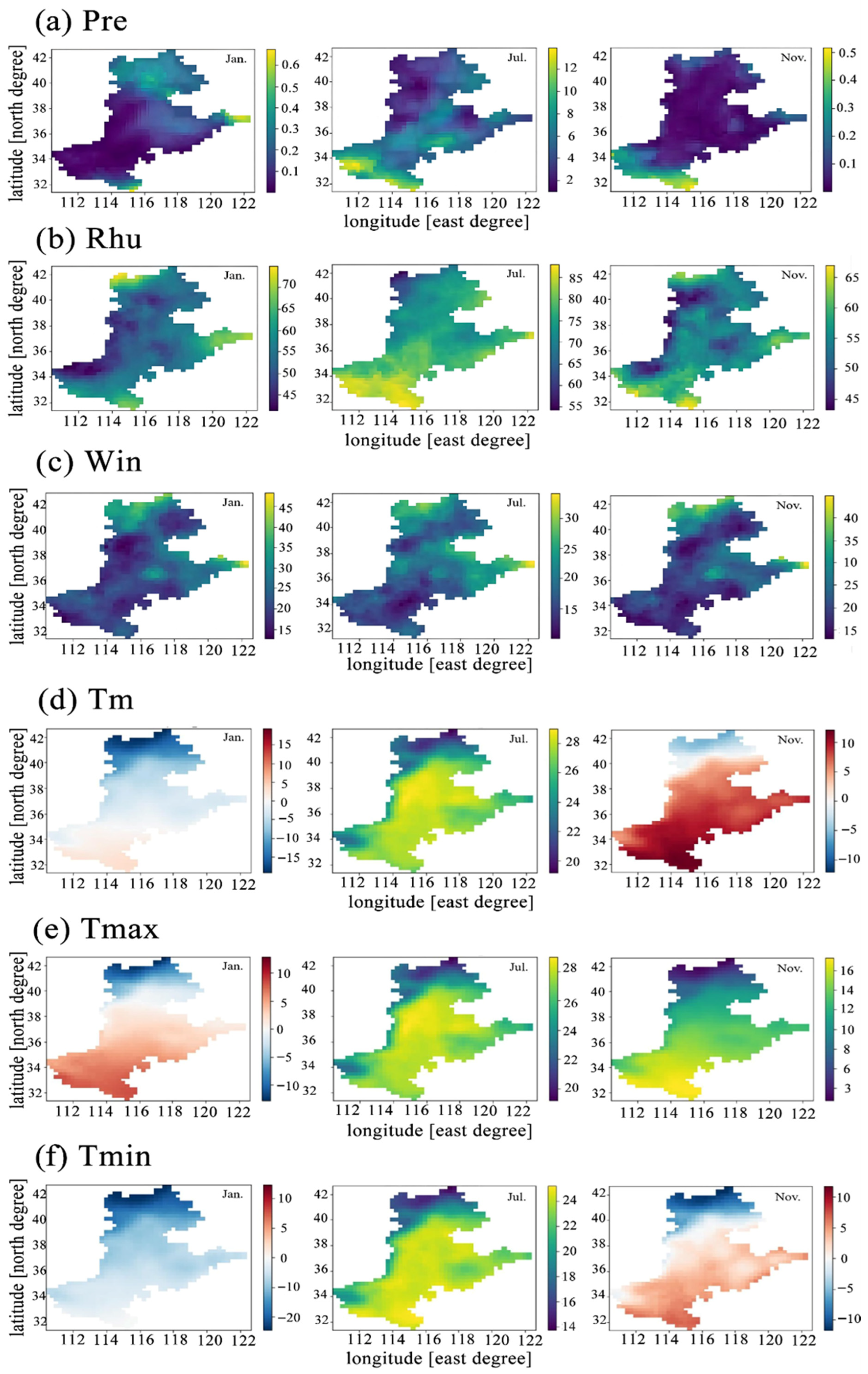
The data of meteorological elements come from the CN05.1 gridded dataset, the interpretation table is shown in Table 1, and the spatial distribution map is shown in Figure 2 and Figure 3. The CN05.1 gridded dataset was obtained from the China Meteorological Data Sharing Network and was used as the observation data [25], with a resolution of 0.25° × 0.25°.
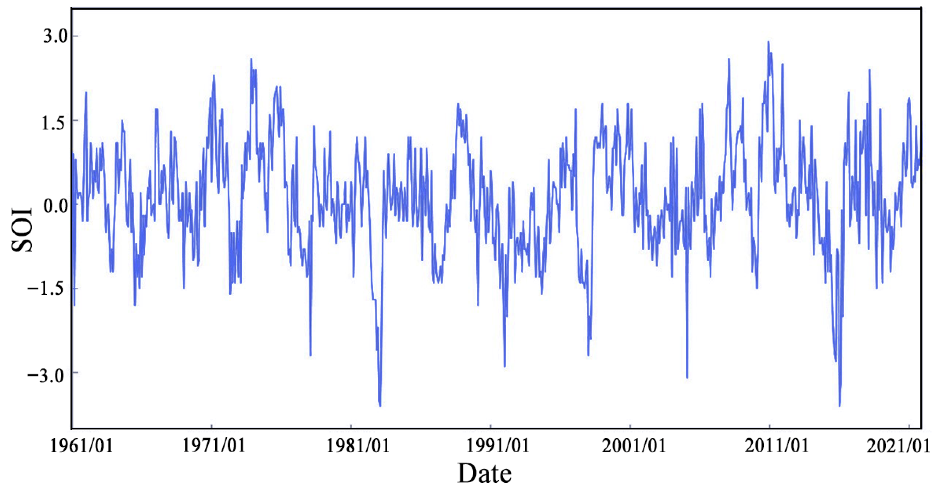
This research selects the Southern Oscillation Index (SOI) as the measure to describe El Niño and La Niña phenomena. The time series plot of SOI is shown in Figure 3. The Southern Oscillation Index (SOI) is a standardized measure of the difference in sea-level pressure between Tahiti and Darwin. It serves as an indicator of the El Niño–Southern Oscillation (ENSO) phenomenon, where negative values correspond to El Niño events and positive values to La Niña events. Monthly SOI data were obtained from the NOAA Climate Prediction Center (CPC) to represent large-scale atmospheric circulation variability affecting precipitation in the Huang–Huai–Hai region.

3. Methods

3.1. Nonparametric Kernel Density Estimation Methods

Kernel density estimation (KDE) is a crucial nonparametric method for estimating the marginal distribution function [26]. KDE emphasizes the calculation of the kernel function and the optimal bandwidth. The Gaussian kernel function is commonly used for kernel density estimation due to its smoothness and differentiability. The specific expression formula is
K x x i h = 1 2 π e x p | x x i | 2 2 h 2
where x i represents the observed value of each sample variable; x represents the mean value; K x represents the kernel function; and h represents the bandwidth, which is always a constant greater than 0.

3.2. Vine Copula

The vine copula method was selected for its superior ability to model nonlinear, asymmetric, and high-dimensional dependencies among meteorological variables, which traditional methods cannot effectively capture. The vine copula function combines a series of trees consisting of nodes and edges. Research scholars have proposed a graphical modeling method called R-Vine (Regular Vine) [27]. A d-dimensional R-Vine is defined by the following conditions:
f x 1 , , x p = f 1 ( x 1 ) f 2 ( x 2 x 1   f p ( x p | x 1 , , x p 1 )
Then f x 1 , , x p can be further decomposed to the following:
f x 1 , , x p = i = 1 p f i x i { i = 2 p j = 1 i 1 c i j | ( j + 1 ) ( i 1 ) ( F ( x i | x j + 1 , , x i 1 ) , F ( x j | x j + 1 , , x i 1 ) ) }
where f i denotes the marginal density of x i , F ( x i | x j + 1 , , x i 1 ) is its univariate conditional distribution function, and c i j | ( j + 1 ) ( i 1 ) is the density of the conditional vine copula associated with the bivariate conditional distribution of x i and x j , given the subset, x j + 1 , , x i 1 .
Due to the non-uniqueness of the probability density function in the R-Vine decomposition expansion form, the number of possible R-Vine compositions for a one-dimensional random variable can be very large. Consequently, two specific vine structures, C-Vine and D-Vine, have garnered attention from scholars. If T i contains only one root node with a degree of d i , where i = 1,2 ,   , d 1 , then this particular structure is referred to as a C-Vine. The joint probability density function can be broken down into its equivalent components.

3.3. Multivariate Joint Change Point Test

The change points detection of multivariables is a measure of the change degree in multivariable dependencies. Unlike univariable and bivariables, the change point detection of multivariables requires Bayesian Information Criterion (BIC) due to its complex internal interdependencies and the uncertainty [28]. The vine copula change point (VCCP) method [23] is introduced to detect the change point in multivariate dependencies. Specifically, adapted binary segmentation (ABS) and wild binary segmentation [29] based on MOving SUM (MOSUM) [30] are selected as two segmentation methods. Vuong [31] and Stationary Bootstrap (SB) [32] are selected as two methods used to perform inference on the candidate change points.

3.4. Total Probability Formula Based Orthogonal Experiments

Orthogonal experiment is a quantitative design analysis method for studying multiple factors and levels [33]. This method is used to detect the factors that have the greatest impact on the dependency structures of multidimensional meteorological factors. However, since the dependence structure between multivariate meteorological factors is asymmetric, i.e., some are positively correlated and some are negatively correlated, the negatively correlated variables should be converted and calculated based on the total probability formula when calculating the joint probability using the copula function. Therefore, we used the total probability formula based orthogonal experiments (TPOE) to detect the most sensitive meteorological factors.
Equation (4) is a typical equation for the orthogonal experiment to calculate the experimental results, i.e., the joint probability density. Equation (4) represents the joint probability equation for 7-dimensional variables without negatively correlated variables. Equation (5) represents the joint probability equation for 7-dimensional variables with two negatively correlated variables.
P X 1 x 1 , , X 7 x 7 = C a , b , d , e , u , v , w
where P X 1 x 1 = F X 1 x 1 ) = a , , P X 7 x 7 = F X 7 x 7 ) = w .
Consequently,
              P X 1 x 1 , X 2 > x 2 , X 3 > x 3 , X 4 x 4 , X 5 x 5 , X 6 x 6 , X 7 x 7 =                 P X 1 x 1 , X 4 x 4 , X 5 x 5 , X 6 x 6 , X 7 x 7 P X 1 x 1 , X 2 x 2 , X 4 x 4 , X 5 x 5 , X 6 x 6 , X 7 x 7 P X 1 x 1 , X 3 x 3 , X 4 x 4 , X 5 x 5 , X 6 x 6 , X 7 x 7 + P X 1 x 1 , X 2 x 2 , X 3 x 3 , X 4 x 4 , X 5 x 5 , X 6 x 6 , X 7 x 7 = C a , e , u , v , w C a , b , e , u , v , w C a , d , e , u , v , w + C a , b , d , e , u , v , w
The 5-dimensional variables include the meteorological factors, Pre, Rhu, Tm, Tmax, and Tmin. The first six-dimensional variables (6-1 dimensional variables) include an additional factor, SOI, compared to the 5-dimensional variables. The second six-dimensional variables (6-2 dimensional variables) include an additional factor, Win, compared to the 5-dimensional variables. The 7-dimensional variables include all meteorological factors.

4. Results

4.1. Multivariate Correlation Analysis and Marginal Distribution Fitting

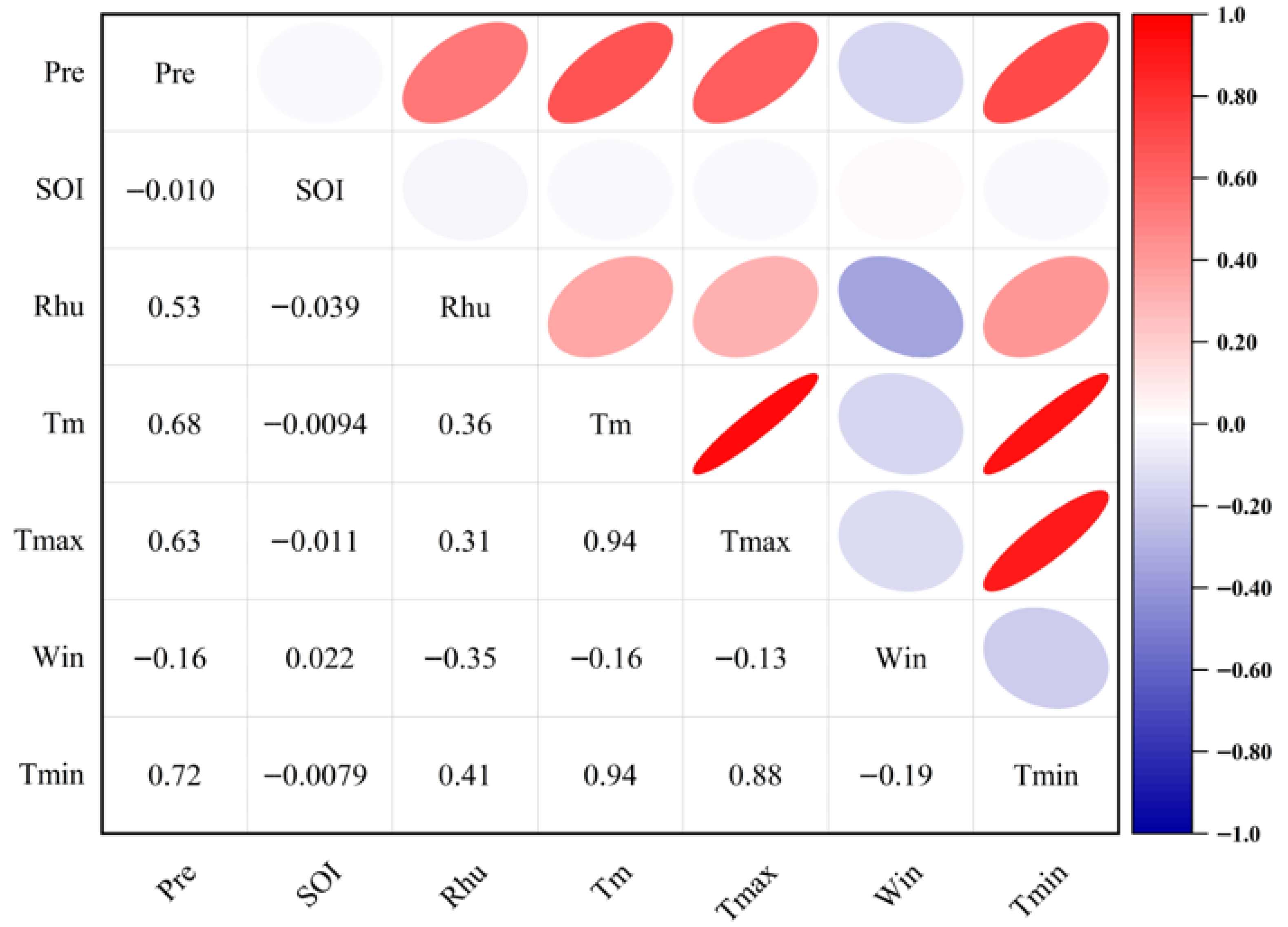
The correlations between precipitation and the other six meteorological factors were tested using the Kendall correlation coefficient, as shown in Figure 4. The Kendall correlation coefficient is not only a measure of dependence [34], but it can also be directly used as the basis for estimating the copula parameter in copula theory [35]. Figure 4 shows an asymmetric dependency structure among the seven variables. For instance, there is a strong positive correlation among the three temperature variables, while Win and SOI are in negative correlation with precipitation.
Four types of distributions, such as Gamma, normal, lognormal, and KDE distributions, were employed to fit these seven variables, and the Kolmogorov–Smirnov (KS) test and Root Mean Squared Error (RMSE) are used as goodness-of-fit tests [36,37]. The results, shown in Table 2, indicate that precipitation’s right-skew and upper-tail mass are best captured by a Gamma margin, while SOI is adequately modeled by a near-symmetric Normal margin. Wind and humidity variables display shapes for which KDE guards against parametric bias. This mix of parametric and non-parametric marginals minimizes the risk that subsequent dependence estimates (and detected change points) are artifacts of marginal misspecification rather than genuine copula-level structure.
The probability density functions used for marginal fitting are expressed as follows:
  • For the Gamma distribution, f ( x ; k , θ ) = 1 Γ ( k ) θ k x k 1 e x θ ,   x > 0 , y > 0 , θ > 0;
  • For the Lognormal distribution, f x ; μ , σ = 1 x σ 2 π exp l n x μ 2 2 σ 2 , x > 0 .
Here, k and θ denote the shape and scale parameters, while μ and σ denote the mean and standard deviation of the logarithmic variable. These formulations provide clear guidance for reproducing the marginal distribution fitting in Table 2.

4.2. Structure and Parameters of Vine Copula

The optimal joint distributions of Pre, Win, Rhu, Tm, Tmax, Tmin, and SOI are selected from R/D/C vine copula functions. The Cramér–von Mises (Cvm) test [38], KS test, the AIC (Akaike Information Criterion) [39], and the BIC are used to test the goodness of fitness of the three vine copula types. The results of goodness of fitness and parameters of vine copula for the 7-dimensional variables are shown in Table 3 and Figure 5. The structures of the other dimensions are shown in Table S1.
According to these testing results, the optimal vine copula functions for the 7-dimensional variables, the 6-1 dimensional variables, the 6-2 dimensional variables, and the 5-dimensional variables are R, R, C, and R-Vine copula, respectively.

4.3. Detection of Change Point for Testing the Non-Stationarity of Multivariables

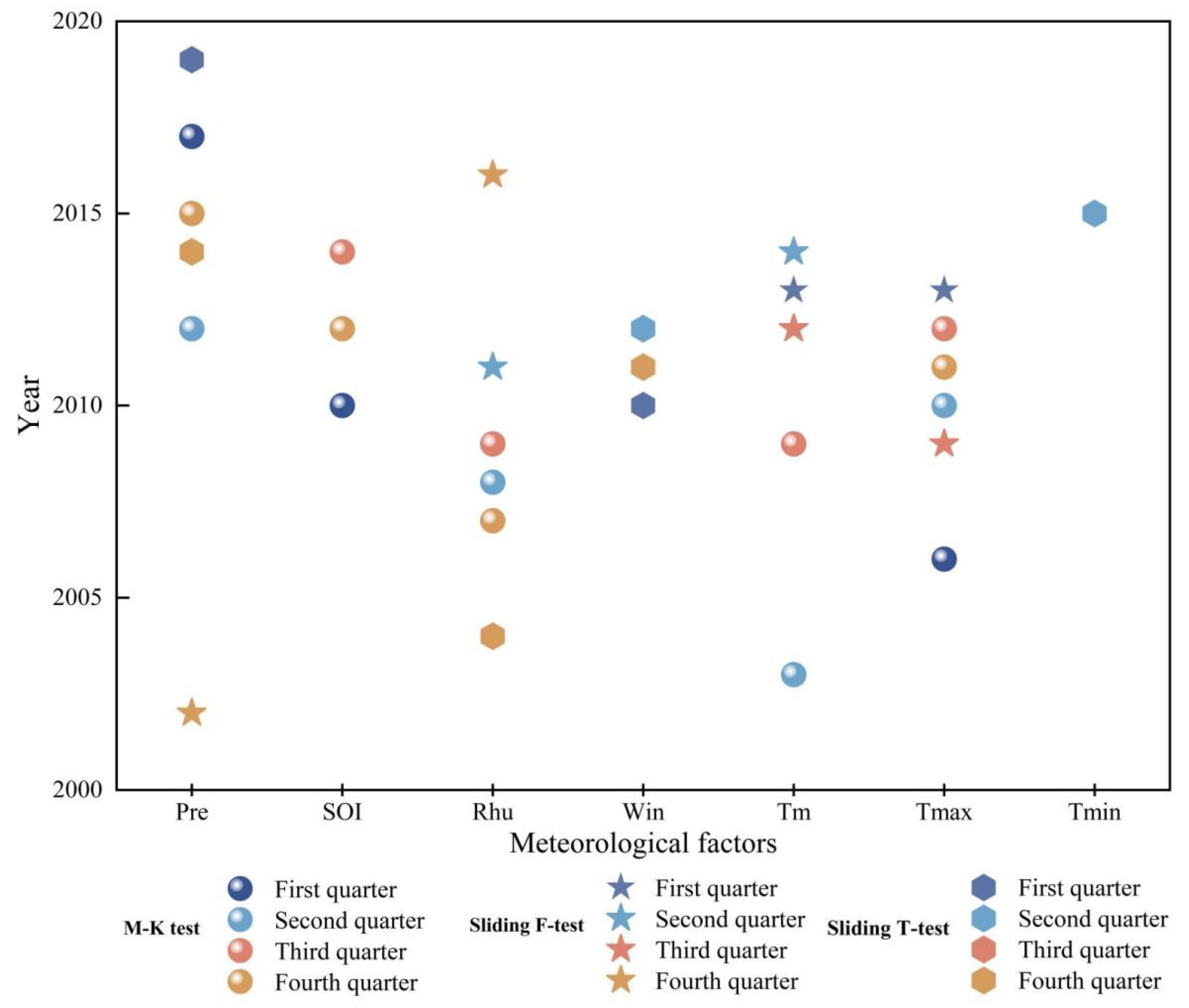
The univariate change point, tested by the Mann–Kendall test [40], sliding F-test, and sliding t-test [41], are shown in Figure 6.
Figure 6 shows that Pre, Rhu, and Tmax are the top three univariate factors with the highest number of change points, while Tmin, Win, and SOI have the fewest change points. The change point of Tmax, Rhu, Pre, SOI, Win and Tm is detected in 2010, 2008, 2015, 2012, 2010, 2013, respectively.
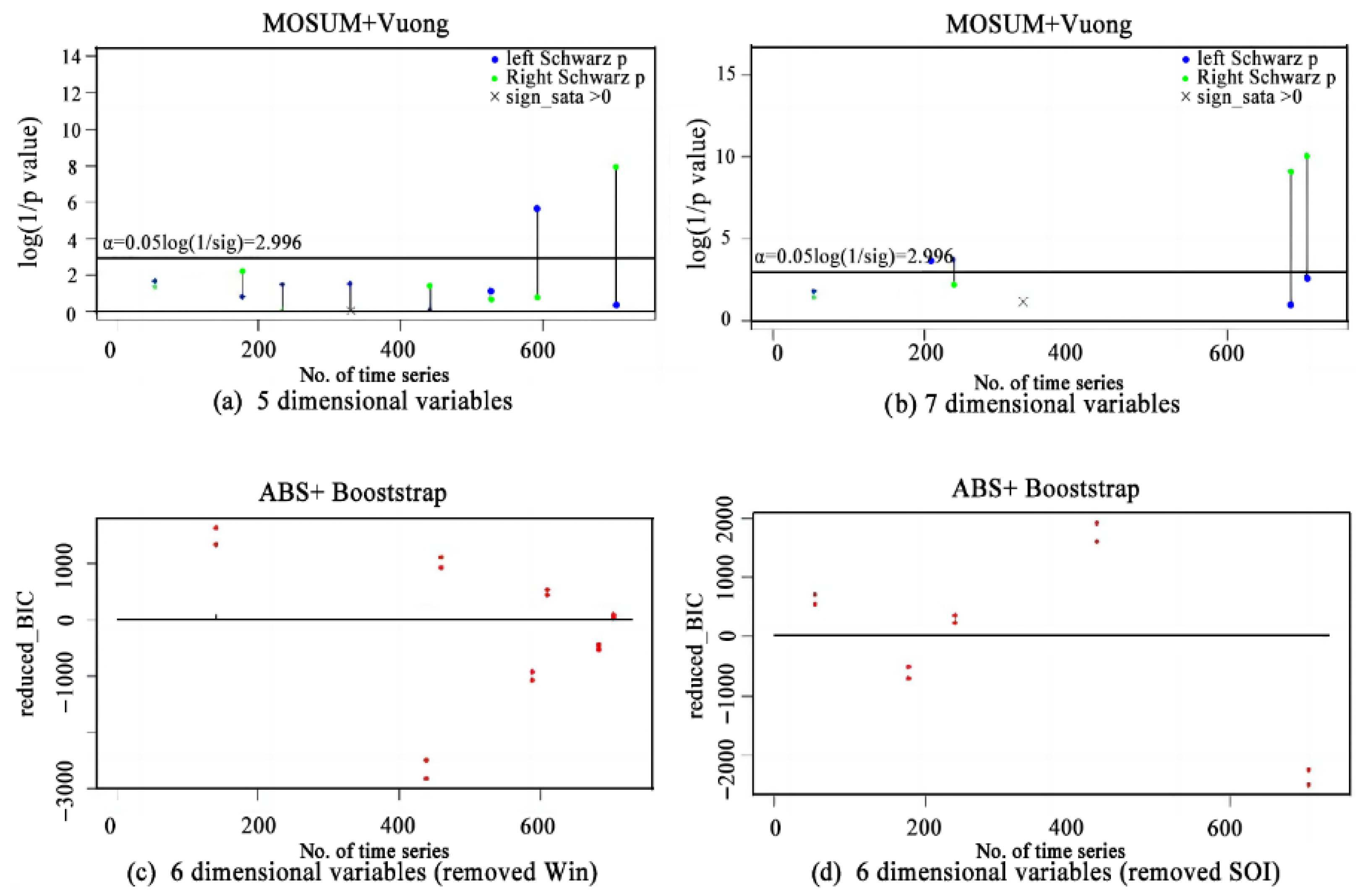
The change point results for the multivariate dependencies are shown in Figure 7. The change points in the dependencies for the 7-variable, 6-variable, and 5-variable are detected in 2017, 2017, and 2018, respectively. Figure 7 indicates that univariate shifts (e.g., in means or variability) tend to precede the detected change points in multivariate dependence (VCCP). This sequencing suggests that drivers may change first, while the reorganization of cross-variable dependence materializes with a lag.
By comparison, it was found that change points in univariate factors typically precede those in multivariate dependencies. Therefore, it is reasonable to assume that changes in single factors may lead to subsequent changes in dependencies.

5. Discussion

To further investigate the driving forces affecting the dependencies between hydrometeorological factors, the driving factors affecting the dependence structure were explored by the law of Total Probability and Orthogonal Experiment Method (TPOEM). An orthogonal experiment with six factors (Tm, Tmax, Tmin, Win, Rhu, and SOI) and three levels was designed (consisting of 18 experimental combinations). The three levels of six variables were divided according to their marginal distributions and the results of the division are shown in Table 4. In order to explore the response of precipitation to the other six meteorological factors, the factor of Pre is divided into nine levels individually, that is, 10, 15, 20, 30, 40, 50, 70, 90, and 130. For each level of the Pre, 18 orthogonal test combinations were evaluated across three temporal windows, the full record, the pre-change period, and the post-change period, yielding 486 experimental cases in total (18 × 9 × 3). The orthogonal experimental design is summarized in Table S2.
Table 5 illustrates the extreme differences in each meteorological factor under orthogonal experiments with varying precipitation frequencies. Based on the extreme difference values, the three meteorological factors Tmin, Win, and Tmax exhibit higher sensitivity to precipitation changes in the Huang-Huai-Hai region. When precipitation fluctuates between 15 and 40 mm, the sensitivity ranking of each meteorological factor is as follows: Tmin > Win > Tmax > Tm > SOI > Rhu. As precipitation increases to 70 to 90 mm, Rhu becomes the most influential factor, indicating that the impact of Rhu on the multivariate joint distribution model intensifies with higher precipitation levels.
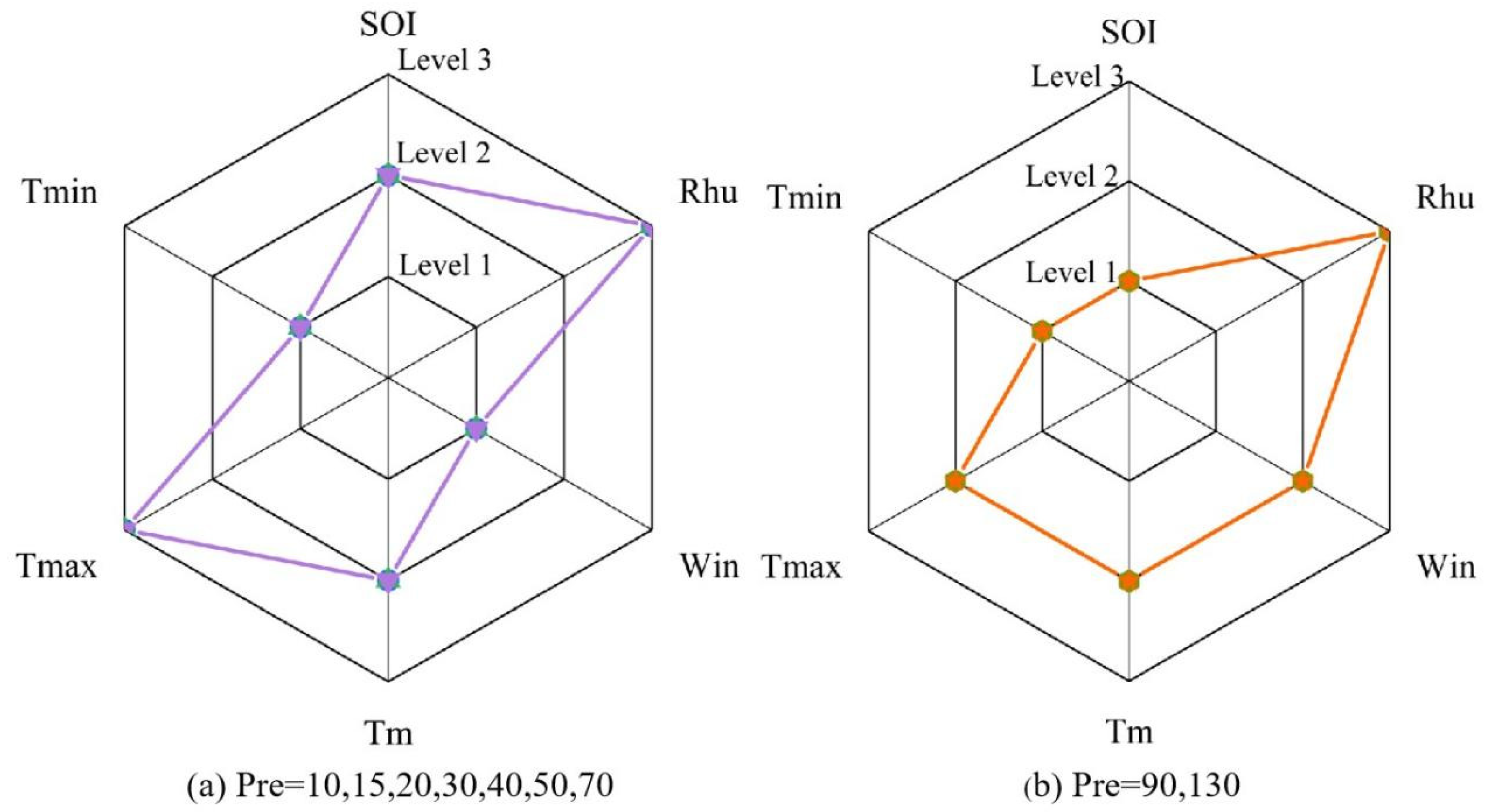
Table 5 ranks the factors by the range of their contributions across levels within each precipitation class in the orthogonal design. Figure 8 then visualizes the level choices for those factors: for each class, we select the level that maximizes the targeted joint-CDF performance (as defined in the TPOE step) following the ranking in Table 5. When two levels tie on performance, we adopt the level associated with the higher-ranked factor combination according to Table 5; if ties persist, we prefer the level that yields the narrower bootstrap spread in the joint-CDF estimate. Thus, Table 5 provides the ranking logic, while Figure 8 encodes the resulting level configuration across precipitation classes. The specific discussion is as follows.
When precipitation varies between 10 and 70 mm, the factors Rhu and Tmax are at level 3, SOI and Tm are at level 2, and Win and Tmin are at level 1. In this range, the multivariate joint distribution model achieves the highest CDF value (Figure 8a). The early flood season in the Huang-Huai-Hai region occurs in June and early July. During this period, the southeast and southwest monsoons influence the region, leading to a continuous increase in average temperatures [42]. Water vapor carried by the East Asian summer winds from the Bay of Bengal, the South China Sea, and the western Pacific Ocean increases the relative humidity in North China, creating a favorable water vapor background for heavy rainfall [43].
When precipitation ranges from 70 to 130 mm, SOI shifts from level 2 to level 1, and Win shifts from level 1 to level 2. In this range, the highest CDF value for the multivariate joint distribution model was observed with these changes (Figure 8b). The main flood season in the Huang-Huai-Hai region occurs in July and August, when the influence of the southeast and southwest monsoons strengthens, maintaining high relative humidity and average temperatures. Unlike the early flood season, the main flood season is marked by frequent ENSO activities [44], resulting in a larger SOI.

6. Conclusions

Exploring the non-stationarity of multidimensional hydrometeorological factors using vine copula not only helps us to understand the change process of the dependencies among hydrometeorological factors, but also provides a conditional probability table (CPT) for constructing machine learning-based meteorological prediction models. Dependencies between the high-dimensional dataset of Pre, Tm, Tmin, Tmax, Win, SOI, and Rhu, in total seven variables, are constructed by vine copula. The VCCP method is introduced to detect the change points of the dependencies between multivariables, and the changes in CDF are analyzed under different variable combinations before and after the change point. Furthermore, the TPOEM is proposed to explore the driving factors affecting the dependence structure, as well as the influence of the six meteorological factors on rainfall under changing environments. The main conclusions are as follows:
(1)
Pre follows a gamma distribution, SOI follows a normal distribution, and Tm, Tmax, Rhu, Win, and Tmin follow the KDE distribution. The R-Vine copula provides the best fit for the multivariate joint distribution.
(2)
Change points in single factors often preceded change points in the joint distribution, indicating that changes in individual factors can influence alterations in the overall joint distribution.
(3)
Tmin, Win, and Tmax exhibit greater sensitivity to variations in precipitation levels in the Huang-Huai-Hai region. As precipitation increases, the influence of Rhu on the multivariate joint distribution intensifies. Higher values of Rhu and Tmax correspond to better CDF values in the multivariate joint distribution. Additionally, higher precipitation values lead to increased SOI values, which in turn result in higher CDF values for the multivariate joint distribution.
Vine copula can more accurately reflect the correlation between hydrometeorological factors. In the Huang-Huai-Hai region, changes in Tmin, Win, and Tmax may have a significant impact on hydrometeorological events. Additionally, this paper proposes a new approach for exploring the comprehensive relationships of hydrometeorological factors in other regions. When applying the framework beyond the HHH region, factor sensitivities should be re-estimated from local data rather than preset. In practice, this means re-fitting the marginals and vine structure, re-detecting dependence change points (VCCP), and re-running the TPOE step to obtain region-specific rankings.

Supplementary Materials

The following supporting information can be downloaded at https://www.mdpi.com/article/10.3390/atmos16111262/s1. Table S1: Structures and parameters of other dimensions; Table S2: Orthogonal experiment grouping table.

Author Contributions

Conceptualization, Y.L.; Data curation, D.J., H.W. and C.H.; Formal analysis, Y.L. and D.J.; Funding acquisition, Y.L.; Investigation, H.W. and G.S.; Methodology, Y.L.; Supervision, G.S.; Visualization, C.H.; Writing—original draft, D.J.; Writing—review and editing, Y.L. and G.S. All authors have read and agreed to the published version of the manuscript.

Funding

This study was supported by a grant from the National Natural Science Foundation of China (No. 42301046), and Natural Science Foundation of Shandong Province (No. ZR202102240660).

Institutional Review Board Statement

Not applicable.

Informed Consent Statement

Not applicable.

Data Availability Statement

Data will be made available on request.

Conflicts of Interest

The authors declare no conflicts of interest.

References

  1. Espinosa, L.A.; Portela, M.M.; Matos, J.P. Climate change trends in a European coastal metropolitan area: Rainfall, temperature, and extreme events (1864–2021). Atmosphere 2022, 13, 1995. [Google Scholar] [CrossRef]
  2. Zhang, W.; Luo, M.; Gao, S. Compound hydrometeorological extremes: Drivers, mechanisms and methods. Front. Earth Sci. 2021, 9, 673495. [Google Scholar] [CrossRef]
  3. He, S.; Wang, H. Oscillating relationship between the East Asian winter monsoon and ENSO. J. Clim. 2013, 26, 9819–9838. [Google Scholar] [CrossRef]
  4. Sun, B.; Wang, H. Interannual variation of the spring and summer precipitation over the three river source region in China and the associated regimes. J. Clim. 2018, 31, 7441–7457. [Google Scholar] [CrossRef]
  5. Park, C.; Son, S.W.; Kim, H. Distinct features of atmospheric rivers in the early versus late East Asian summer monsoon and their impacts on monsoon rainfall. J. Geophys. Res. Atmos. 2021, 126, e2020JD033537. [Google Scholar] [CrossRef]
  6. Sun, Y.; Li, J. Synergistic effect of El Niño and the North Pacific Oscillation on wintertime precipitation over southeastern China and the East China Sea Kuroshio area. Clim. Dyn. 2022, 58, 1635–1649. [Google Scholar] [CrossRef]
  7. Zeng, Y.; Yang, L. Triggering mechanism of an extreme rainstorm process near the Tianshan Mountains in Xinjiang, an arid region in China, based on a numerical simulation. Adv. Meteorol. 2020, 2020, 8828060. [Google Scholar] [CrossRef]
  8. Sun, B.; Wang, H.; Zhou, B.; Li, H.; Zhu, B. A review on the interannual and interdecadal variations of water vapor transport over China during past decades. Water Resour. Prot. 2020, 31, 644–653. [Google Scholar]
  9. Fan, Z.X.; Thomas, A. Decadal changes of reference crop evapotranspiration attribution: Spatial and temporal variability over China 1960–2011. J. Hydrol. 2018, 560, 461–470. [Google Scholar] [CrossRef]
  10. Shi, Z.; Zhou, P.; Li, X.; Cheng, H.; Sha, Y.; Xie, X.; Liu, H.; Wu, J.; Liu, X. Distinct Holocene precipitation trends over arid Central Asia and linkages to westerlies and Asian monsoon. Quat. Sci. Rev. 2021, 266, 107055. [Google Scholar] [CrossRef]
  11. Wang, R.; Zhang, X.; Guo, E.; Cong, L.; Wang, Y. Characteristics of the spatial and temporal distribution of drought in Northeast China, 1961–2020. Water 2024, 16, 234. [Google Scholar] [CrossRef]
  12. Gleason, J.A.; Kratz, N.R.; Greeley, R.D.; Fagliano, J.A. Under the weather: Legionellosis and meteorological factors. EcoHealth 2016, 13, 293–302. [Google Scholar] [CrossRef]
  13. Poornima, S.; Pushpalatha, M. Prediction of rainfall using intensified LSTM based recurrent neural network with weighted linear units. Atmosphere 2019, 10, 668. [Google Scholar] [CrossRef]
  14. Sadeghi, M.; Asanjan, A.A.; Faridzad, M.; Nguyen, P.; Hsu, K.; Sorooshian, S.; Braithwaite, D. PERSIANN-CNN: Precipitation estimation from remotely sensed information using artificial neural networks–convolutional neural networks. J. Hydrometeorol. 2019, 20, 2273–2289. [Google Scholar] [CrossRef]
  15. Grange, S.K.; Lewis, A.C.; Carslaw, D.C. Source apportionment advances using polar plots of bivariate correlation and regression statistics. Atmos. Environ. 2016, 145, 128–134. [Google Scholar] [CrossRef]
  16. Lin, W.; Song, S. Calculation method of joint probability for flood based on mixed Copula function. J. Hydraul. Eng. 2021, 40, 40–51. [Google Scholar]
  17. Achite, M.; Bazrafshan, O.; Wałęga, A.; Azhdari, Z.; Krakauer, N.; Caloiero, T. Meteorological and hydrological drought risk assessment using multi-dimensional copulas in the Wadi Ouahrane Basin in Algeria. Water 2022, 14, 653. [Google Scholar] [CrossRef]
  18. Yang, X.; Li, Y.; Huang, G.; Li, Y.; Liu, Y.; Zhou, X. Development of a multi-GCMs Bayesian copula method for assessing multivariate drought risk under climate change: A case study of the Aral Sea basin. Catena 2022, 212, 106048. [Google Scholar] [CrossRef]
  19. Zavareh, M.M.; Mahjouri, N.; Rahimzadegan, M.; Rahimpour, M. A drought index based on groundwater quantity and quality: Application of multivariate copula analysis. J. Clean. Prod. 2023, 417, 137959. [Google Scholar] [CrossRef]
  20. Razmkhah, H.; Fararouie, A.; Ravari, A.R. Multivariate flood frequency analysis using bivariate copula functions. Water Resour. Manag. 2022, 36, 729–743. [Google Scholar] [CrossRef]
  21. Yang, R.; Wu, S.Q.; Gao, X.P.; Zhang, C. A vine copula-based study on identification of multivariate water environmental risk under different connectivity of rivers and lakes. J. Hydraul. Eng. 2020, 51, 606–616. [Google Scholar] [CrossRef]
  22. Song, S.; Wu, Y.H.; Xu, B.S.; Wu, G.; Zhang, J. Pair copula technique of seismic vulnerability assessment of cable-stayed bridge system. Mech. Eng. 2021, 38, 110–123. [Google Scholar]
  23. Xiong, X.; Cribben, I. Beyond linear dynamic functional connectivity: A vine copula change point model. J. Comput. Graph. Stat. 2022, 32, 853–872. [Google Scholar] [CrossRef]
  24. Smeenk, M.L.W.J.; Agramunt, J.; Bonger, K.M. Recent developments in bioorthogonal chemistry and the orthogonality within. Curr. Opin. Chem. Biol. 2021, 60, 79–88. [Google Scholar] [CrossRef]
  25. Wu, J.; Gao, X. A gridded daily observation dataset over China region and comparison with the other datasets. Chin. J. Geophys. 2013, 56, 1102–1111. [Google Scholar] [CrossRef]
  26. Parzen, E. On estimation of a probability density function and mode. Ann. Math. Stat. 1962, 33, 1065–1076. [Google Scholar] [CrossRef]
  27. Czado, C.; Jeske, S.; Hofmann, M. Selection strategies for regular vine copulae. J. Société Française Stat. 2013, 154, 174–191. [Google Scholar]
  28. Czado, C.; Nagler, T. Vine copula based modeling. Annu. Rev. Stat. Appl. 2022, 9, 453–477. [Google Scholar] [CrossRef]
  29. Fryzlewicz, P. Wild binary segmentation for multiple change-point detection. Ann. Stat. 2014, 42, 2243–2281. [Google Scholar] [CrossRef]
  30. Eichinger, B.; Kirch, C. A MOSUM procedure for the estimation of multiple random change points. Bernoulli 2018, 24, 526–564. [Google Scholar] [CrossRef]
  31. Vuong, Q.H. Likelihood ratio tests for model selection and non-nested hypotheses. Econometrica 1989, 57, 307–333. [Google Scholar] [CrossRef]
  32. Politis, D.N.; Romano, J.P. The stationary bootstrap. J. Am. Stat. Assoc. 1994, 89, 1303–1313. [Google Scholar] [CrossRef]
  33. Liu, L.H.; Zhang, Q.W.; Wang, Y.D.; Gu, X. Research progress on heavy metal migration model at watershed scale. China Environ. Sci. 2023, 43, 4229–4238. [Google Scholar]
  34. Gijbels, I.; Veraverbeke, N.; Omelka, M. Conditional copulas, association measures and their applications. Comput. Stat. Data Anal. 2011, 55, 1919–1932. [Google Scholar] [CrossRef]
  35. Nazeri Tahroudi, M.; Ramezani, Y.; de Michele, C.; Mirabbasi, R. Multivariate analysis of rainfall and its deficiency signatures using vine copulas. Int. J. Climatol. 2022, 42, 2005–2018. [Google Scholar] [CrossRef]
  36. Fasano, G.; Franceschini, A. A multidimensional version of the Kolmogorov–Smirnov test. Mon. Not. R. Astron. Soc. 1987, 225, 155–170. [Google Scholar] [CrossRef]
  37. Chai, T.; Draxler, R.R. Root mean square error (RMSE) or mean absolute error (MAE). Geosci. Model Dev. 2014, 7, 1525–1534. [Google Scholar] [CrossRef]
  38. Neuhaus, G. Asymptotic power properties of the Cramér–von Mises test under contiguous alternatives. J. Multivar. Anal. 1976, 6, 95–110. [Google Scholar] [CrossRef]
  39. Chakrabarti, A.; Ghosh, J.K. AIC, BIC and recent advances in model selection. In Philosophy of Statistics; Elsevier: Amsterdam, The Netherlands, 2011; pp. 583–605. [Google Scholar] [CrossRef]
  40. Hamed, K.H.; Rao, A.R. A modified Mann–Kendall trend test for autocorrelated data. J. Hydrol. 1998, 204, 182–196. [Google Scholar] [CrossRef]
  41. Dong, Y.; Wang, J.; Jiang, H.; Shi, X. Intelligent optimized wind resource assessment and wind turbines selection in Huitengxile of Inner Mongolia, China. Appl. Energy 2013, 109, 239–253. [Google Scholar] [CrossRef]
  42. Ling, M.; Han, H.; Hu, X.; Xia, Q.; Guo, X. Drought characteristics and causes during summer maize growth period on Huang-Huai-Hai Plain based on daily scale SPEI. Agric. Water Manag. 2023, 280, 108198. [Google Scholar] [CrossRef]
  43. Xie, T.; Huang, W.; Chang, S.; Zheng, F.; Chen, J.; Chen, J.; Chen, F. Moisture sources of extreme precipitation events in arid Central Asia and their relationship with atmospheric circulation. Int. J. Climatol. 2021, 41, E271–E282. [Google Scholar] [CrossRef]
  44. Wang, L.; Wang, J.; He, F.; Wang, Q.; Zhao, Y.; Lu, P.; Huang, Y.; Cui, H.; Deng, H. Spatial–temporal variation of extreme precipitation in the Yellow–Huai–Hai–Yangtze Basin of China. Sci. Rep. 2023, 13, 9312. [Google Scholar] [CrossRef] [PubMed]
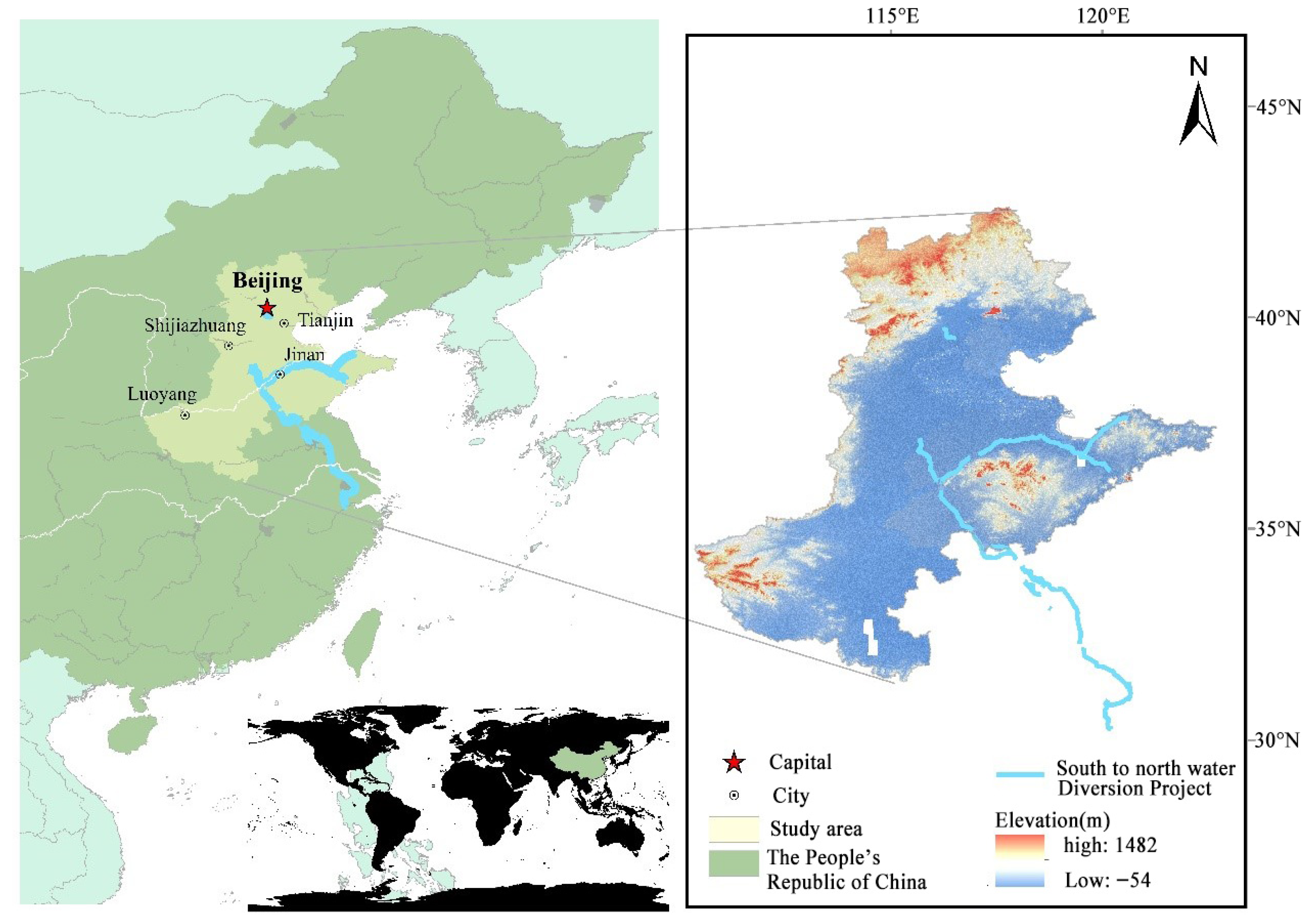
Figure 1. The location and elevation of Huang-Huai-Hai region.
Atmosphere 16 01262 g001
Figure 2. Spatial distribution of Pre, Rhu, Win, Tm, Tmax, and Tmin in CN05.1 grid dataset.
Atmosphere 16 01262 g002
Figure 3. Time series plot of SOI.
Atmosphere 16 01262 g003
Figure 4. Heat map of correlation among seven meteorological factors.
Atmosphere 16 01262 g004
Figure 5. The structure and parameters of vine copula of 7 variables. (1 represents Pre, 2 represents 7SOI, 3 represents Rhu, 4 represents Win, 5 represents Tm, 6 represents Tmax, 7 represents Tmin).
Atmosphere 16 01262 g005
Figure 6. Results of mutation test for seven meteorological factors.
Atmosphere 16 01262 g006
Figure 7. VCCP combined change point detection map.
Atmosphere 16 01262 g007
Figure 8. Distribution of optimal levels of different meteorological factors.
Atmosphere 16 01262 g008
Table 1. CN05.1 data factor interpretation table.
FactorConnotationUnitFactorConnotationUnit
PrePrecipitation mmTminMinimum daily temperature°C
TmAverage temperature°CWinMean wind speedm/s
TmaxMaximum daily temperature°CRhuRelative humidity%
Table 2. Marginal distribution of seven factors.
Meteorological FactorGamma DistributionNormal
Distribution
Log-Normal Distribution KDE
Distribution
K-S Test
Boundary
Values
Pre(0.9117, 59.1133)(53.8931, 54.6152)(3.3468, 1.3005)h = 10.52990.0515
0.04570.16330.06270.0860
SOI/(0.1098, 1.0091)/h = 0.254469
0.0412, 0.01700.0391, 0.0182
Rhu(41.9012, 1.5416)(64.5934, 9.8813)(4.1561, 0.1561)h = 3.22985
0.0429, 0.02270.0452, 0.02490.0442, 0.58350.0271, 0.0090
Win(19.9033, 0.1286)(2.5586, 0.5930)(0.9141, 0.2228)h = 0.164217
0.06030.07850.0505, 0.02560.0264, 0.0097
Tm(1.6843, 7.3195)(11.7905, 10.2552)/h = 4.09806
0.22320.12430.0505
Tmax(3.0909, 5.7196)(17.6689, 10.0729)(2.4382, 1.8716)h = 3.88532
0.17120.13230.35410.0508
Tmin/(6.8733, 10.1775)/3.98215
0.1156 0.0497
Note: Means and variances of the distributions are in parentheses in the first row, and KS test and RMSE test values are in the second row; the KDE distribution h is the bandwidth, and the kernel function is Normal; the bolded portion represents a good fit to the marginal distribution.
Table 3. Seven vine copula preference test table.
Variable
Combinations
Vine Copula
Types
CvmCvm PKSKS PAICBIC
7-dimensional variablesR-Vine0.01230.99380.73270.7385−11,615.21−11,514.11
D-Vine0.03060.91630.85910.7385−11,478.7−11,372.99
C-Vine0.01251.00000.72280.8372−11,629.8−11,528.69
6-1 dimensional variablesR-Vine0.04230.93250.91030.9205−10,901.18−10,832.24
D-Vine0.03520.91251.24710.5103−10,901.18−10,832.24
C-Vine0.06320.56751.56730.416−10,560.46−10,491.53
6-2 dimensional variablesR-Vine0.05810.84381.09310.7713−11,593.14−11,519.6
D-Vine0.05430.54381.39220.6038−11,609.95−11,541.02
C-Vine0.03470.99130.87380.9300−11,611.81−11,538.28
5-dimensional variablesR-Vine0.05070.88751.70380.4688−10,879.82−10,833.86
D-Vine0.15340.77251.32290.8295−10,879.82−10,833.86
C-Vine0.18930.50382.01860.5200−10,544.38−10,498.42
Note: Cvm P and KS P are standard values. When Cvm and KS are less than their respective standard values, the test passes.
Table 4. Factor level table for orthogonal experiments.
SOIRhu
(%)
Win
(m/s)
Tm
(°C)
Tmax
(°C)
Tmin
(°C)
Pre
(mm)
Level 1−0.556.812.092.428.32−2.19103070
CDF Values0.2680.25310.25940.24980.24720.25710.18930.44280.7283
Level 20.163.922.4312.9119.427.5154090
CDF Values0.49250.49340.4930.50250.51340.50530.26350.53550.8091
Level 30.872.022.8821.6827.6616.412050110
CDF Values0.75210.74070.74410.76890.77750.76080.32960.61200.9052
Table 5. The results of the orthogonal experiment.
Pre
(mm)
RangeRanking of Impact
SOIRhuWinTmTmaxTmin
103258.84 3160.43 3301.87 3333.17 3530.88 3675.17 Tmin > Tmax > Tm > Win > SOI > Rhu
15925.32 920.72 1094.76 1020.97 1091.47 1195.18 Tmin > Win > Tmax > Tm > SOI > Rhu
201672.58 1658.12 1904.06 1805.52 1882.83 2037.00 Tmin > Win > Tmax > Tm > SOI > Rhu
303031.47 2933.94 3375.74 3185.02 3261.16 3529.29 Tmin > Win > Tmax > Tm > SOI > Rhu
403766.26 3529.62 4180.83 3863.63 3945.85 4278.19 Tmin > Win > Tmax > Tm > SOI > Rhu
503843.26 3544.47 4232.92 3831.04 3935.80 4220.70 Win > Tmin > Tmax > SOI > Tm > Rhu
702284.45 4021.97 2725.68 2272.93 2448.92 4409.38 Tmin > Rhu > Win > Tmax > SOI > Tm
902327.19 2833.38 2349.73 1105.99 2196.39 3047.03 Tmin > Rhu > Win > SOI > Tmax > Tm
1302373.34 2279.27 2796.66 512.88 2624.83 2406.64 Win > Tmax > Tmin > SOI > Rhu > Tm
Disclaimer/Publisher’s Note: The statements, opinions and data contained in all publications are solely those of the individual author(s) and contributor(s) and not of MDPI and/or the editor(s). MDPI and/or the editor(s) disclaim responsibility for any injury to people or property resulting from any ideas, methods, instructions or products referred to in the content.