Atmospheric Black Carbon Evaluation in Two Sites of San Luis Potosí City During the Years 2018–2020

Abstract

Nevertheless, there is a lot to know about air pollutants in Mexico’s largest cities, like San Luis Potosi City, which is one of the 12 most crowded cities and is expected to grow in the next years; however, there is little information about air pollutant levels mainly particulate matter in their regulated size fractions (PM₁₀ or PM_2.5), and its main component of the Organic fraction: Black Carbon (BC), which is especially important because of its chemical properties and their effects on human health, air pollution, and climate change. This work presents a one-year BC monitoring in the northern part of the city (2018–2019) and another one-year BC monitoring in the southern area (2019–2020) during the health contingency situation due to the SARX-CoV-2 virus to obtain direct equivalent black carbon (eBC) concentrations and their main fractions related to fossil fuel and biomass burning using aethalometer AE-33, as well as other air pollutants concentrations measured at the same periods by the governmental local monitoring network (SEGAM). At the North, BC mass annual average concentration was (1.11 µg m⁻³), divided into seasonal stations, the cold season was the highest with (1.44 µg m⁻³), followed by the dry season (1.23 µg m⁻³), rainy season (0.94 µg m⁻³) and finally warm dry season (0.83 µg m⁻³). In the south, BC annual average concentration was (1.96 µg m⁻³); divided into seasons, the highest was the dry season with (2.73 µg m⁻³), followed by the cold season (2.37 µg m⁻³), dry warm season (1.61 µg m⁻³) and the rainy season (1.28 µg m⁻³). One of the main findings was the dominance of annual mean concentrations of BC originating from fossil fuels (BCff) on the north site in the city was 0.97 and on the south site (BCff) was 0.91 due to some forest fires during the monitoring period. This study presented information from two zones of a growing city in Mexico to generate new air pollutant indicators to have a better understanding of pollutant interactions in the city, to decrease the emission precursor sources, and reduce the health risks in the population.

1. Introduction

Air pollution in cities has recently become the most significant environmental risk factor for human health all over the world. Ambient Air Pollution (outdoor and indoor) was estimated to cause more than 7 million premature deaths worldwide yearly [1]. In 2021, the WHO considered Particulate Matter (PM), the highest-impact air pollutant, to have adverse effects on human health, especially in the respiratory and cardiovascular systems [2]. Worldwide epidemiological particulate matter studies have reported a substantially increased risk of mortality and morbidity in both; short-term (hourly/daily) and long-term (monthly, yearly, or over time) in the urban population associated with increased ambient PM.

Particulate Matter describes solid or liquid particles (<50 µm) of carbonaceous and inorganic compounds emitted and dispersed into the atmosphere and usually is classified according to their aerodynamic diameter length. PM_2.5 or fine fraction are particles with an aerodynamic diameter of less than 2.5 µm. PM’s main composition can be divided for chemical characterization into inorganic and carbonaceous fractions. This complex heterogeneous mixture of chemical compounds can vary, react with gases and biological compounds, and change depending on thermodynamic properties, and meteorological conditions [3], and according to their main natural or anthropogenic emission sources, can produce one short-lived climate pollutant (SLCP) named Black Carbon (BC), who has a direct negative effect on global climate change [4]. The carbonaceous aerosols in the atmosphere come as a complex mixture of semi-volatile compounds such that they can exist as both condensed in PM and as gases, their major particulate components are generally classified into two categories: Organic Carbon (OC) and Elemental Carbon (EC) which can be associated with BC, depending on their measuring principle.

BC is emitted primarily from the incomplete combustion of fossil fuels, biofuel, and biomass burning [5], can be classified into two subfractions: fossil carbon, which always comes from anthropogenic activities [6], also named fossil fuel Black Carbon (BCff) and biogenic carbon or contemporary carbon or biomass burning Black Carbon (BCbb). Additionally, BC is formally defined as a refractory light-absorbing substance composed of aggregated carbon spherules [7,8], with a strong adsorbability [9], which is identified as an important factor in atmospheric chemical reactions [10] due to its large surface area and physical properties and is always emitted with other particles and gases. It can also act as a substrate or catalyst for various chemical processes [11]. Other effects include urban haze formation, reducing atmospheric visibility [12], changing cloud properties [13], decreasing the production of snow, modifying ice cover processes, and stunting plant growth by adhering to plant surface [14], these adverse impacts have been frequently pointed out in local, regional and global ecosystems. Most importantly, BC is a short-lived climate forcer/pollutant that contributes to climate change by absorbing solar radiation by having a warming potential at least 460 times higher than carbon dioxide equivalent unit (CO₂eq), which causes a negative radiative force [15]. Also, is associated with other compounds emitted in the combustion process just as carbon monoxide (CO), methane (CH₄), CO₂, and OC, producing secondary effects in the global climate and with other air toxic pollutants (like: nitrogen oxides (NOx), sulfur dioxide (SO₂), Volatile Organic Compounds (VOCs), Polycyclic Aromatic Hydrocarbons (PAHs), dioxins, furans, precursors of tropospheric Ozone), alter the different PM formation processes which impact on air quality and human health [16], because of that BC has become one of the key targets for current mitigation strategies and emission control policies all over the world.

The International Agency for Research on Cancer (IARC) classified PM_2.5 as a leading cause of cancer, especially trachea, bronchus, and lung cancer [17]. The fine fraction can cause the most substantial human health impacts. It is associated with delayed psychomotor development and lower child intelligence, may complicate or exacerbate many other adverse health conditions [18,19], and is associated with systemic inflammatory markers and other cardiovascular issues [20]. Other studies have increased their interest in characterizing the contained chemical species present in BC and concluded that some components play a more substantial role in health effects [21,22,23,24], than other carbonaceous aerosols [25,26,27,28,29]. In 2011, Janssen calculated an increment of life expectancy due to a reduction of BC in PM_2.5, associated with the high health risk dominated by these primary combustion particles. However, there is no ambient air quality standard for BC in any country [30].

Air pollution studies have focused on chemical speciation in each PM fraction pollutant. For this reason, Black Carbon or Equivalent black carbon (eBC, when BC data is derived from optical absorption methods) [31] and other carbonaceous or ultrafine aerosols networks have been established worldwide, in North America, Europe, and Asia [32,33,34,35,36] to evaluate different emission sources, make a comparison among various types of sites or cities to create mitigation strategies and establish benchmarks and public policies.

Mexico is number 13 on the list of countries with the largest volumes of CO₂ emissions in the year 2013 (436 Mt CO₂; 1.37% of the global contribution), according to the National Inventory of Greenhouse Gas Emissions in 2018 (INEGEI, its acronym in Spanish) [36]. Also, the INEGEI determined that BC emissions reached nearly 125 million tons, mostly from activities in the transport sector and industry (38%). Hence, Mexico has established the Intended Nationally Determined Contribution (INDC) program to reduce national emissions of BC in mitigation unconditional goals for the following years, so Mexico’s Government expects to reduce around 51% of the BC emissions by the year 2030. As mentioned in the COP21 Conference of the Parties, United Nations Framework Convention on Climate Change. However, there is not enough information or official information on BC measures around the country; consequently, it is necessary to develop mitigation and adaptation strategies, lines of action, etc., but firstly, it is crucial to create accurate measurements to quantify this pollutant and not just factor emissions evaluations.

In Mexico, there is still a lack of information on the concentrations of BC emitted in the vast majority of medium-sized cities. San Luis Potosi Metropolitan Area (SLPMA) has been well known for its metallurgical and mining activities for more than 400 years, and it was established as one of the leading mining zones in the country. Different metals such as gold and silver were extracted, and more recently, copper, zinc, iron, lead, and other sub-product metals were also extracted. Nowadays, its industrial zone has more than 250 manufacturing industries located in an area of about 20 km² south of the city. For this reason, high concentrations of heavy metals such as lead, arsenic, and zinc have been reported surrounding the industrial zone [37], but also all over the city as other studies have shown previously [38,39,40,41].

Industrial wastes have been detected with high concentrations of calcium sulfate and fluorite [42] near ex-mining zones on the west and the east of SLPMA; there are more than 20 environmental liabilities with different kinds of metal composition. In the northwest, it is one of the largest zinc plants in Latin America. It also has a sulfuric acid plant and generates other metals as sub-products. There are more than 100 brick kilns all over the NE zone with minimum control or poorly verified, and because of that, they burn all kinds of waste such as plastics, wood, coke, or even electronic waste. In the south, there are the two main industrial zones, which include foundries, chemical and metallurgical industries, construction activities, and the main avenue named 57th Avenue, which transports nearly 20% of the population from the San Luis Potosí city through the industrial zones every day and is used by the passenger transport but also by the freight and merchandise transport [42]. Other significant sources include two power plants, the food industry, and traffic dust resuspension in paved and unpaved roads.

The latest San Luis Potosí emission inventory for the year 2011 [43], reports about 3329 Mg year⁻¹ for PM₁₀ and 2302 Mg year⁻¹ for PM_2.5 for San Luis Potosí City plus Soledad de Graciano y Sánchez (for this paper, it will be referred as San Luis Potosi Metropolitan Area). As with many current national inventories, information about the different chemical species of particulate matter is not included or even evaluated. According to government data, SLPMA is growing, as are its industrial activities and mobile sources, which highlights the importance of evaluating the primary air pollutants. Furthermore, in the last years, there has been a significant increase in the number of cardiovascular and respiratory diseases associated with different kinds of cancer.

This study evaluated BC hourly concentrations and other associated air pollutants for one year of monitoring from October 2018 to October 2019 in the northeast of San Luis Potosi City and another year in the south zone from November 2019 to November 2020 to evaluate the different impacts that each zone produces in San Luis Potosi city.

2. Materials and Methods

San Luis Potosi City is located in the central zone of Mexico and represents the country’s 11th most crowded metropolitan area (SLPMA), covering nearly 1800 km² and about 1.25 million inhabitants. Population density is almost 700 inhab km⁻² [44]. It is located at an average altitude of 1864 m above sea level (asl), in a semi-arid climate at the central portion of two mountain ranges: at the Northwest side, there is the Sierra de San Miguelito, and at the East, the Sierra de Alvarez.

The first year’s SLPMA monitoring site was the “Estación Biblioteca” (BIB) from the Department of Ecology and Environmental Management (SEGAM, for its acronym in Spanish), at 22°10′34″ N and 100°59′22″ W, in the northeast of the city. This monitoring station is a suburban site with low vehicular density, regular diesel bus density, and a one-rail train with moderate pollutants emission. Still, the main impact is a zone with more than 100 brick kilns.

The monitoring site for the second evaluation year was the “Facultad de Ciencias Sociales y Humanidades de la Universidad Autónoma de San Luis Potosi” (FCSYH) located at 22°8′24″ N and 100°57′01″ W, in the southwest of the city, who is a suburban site, with high vehicular density, high diesel transportation density and a high industrial emission at the zone. Figure 1. shows the monitoring sites location and the main industries in the city according to the National Statistical Directory of Economic Units (DENUE, by its acronym in Spanish), from 2021.

The atmospheric circulation in this partial basin is produced by synopsis circulation during winter, which produces cold fronts propagated through the plains of the central-southeast region of the USA in a cyclonic motion. Additionally, local air effects are produced by a mountain-valley circulation regional easterly winds and a recirculation effect through the urban area that is unfavorable for the dispersion and transport of atmospheric PM beyond downtown [41].

2.1. Sampling

This first sampling campaign was designed to measure PM₁₀ and BC using monitoring automatic equipment each hour for a one-year period at a north zone of SLPMA, evaluate the different kinds of sources near the monitoring site, and observe the emission variation during seasons. A collected sampling base measured PM₁₀ and BC automatic concentrations from 10 October 2018 to 30 October 2019.

The Aethalometer AE-33 (Magee Scientific Company, Ljubljana, Slovenia) measures eBC from the relation of absorption coefficient by measuring the attenuation of incident light transmitted through the sample spots on the filter in a defined mass absorption cross section (MAC) of 16.6 m² g⁻¹ [45]. The AE-33 collected and analyzed PM_2.5 by using a cut point cyclone on a quarter filter type and measured absorption of light at seven wavelengths (370, 470, 520, 590, 660, 880, and 950) nm, on two sample spots simultaneously and combined the concentrations measurements in real-time [46]. In this study, the AE-33 set the flow rate at 5 L min⁻¹, and BC concentrations were collected at the 880 nm channel with a 1 min time resolution and averaged hourly for data analysis and separating directly fossil fuel emissions from biomass burning emissions according to the Carbonaceous Aerosol Analysis Tool software explained in the user manual for the AE-33.

The PM₁₀ measurement was carried out with the Beta Attenuation Monitor equipment (BAM), a property of the SEGAM. The BAM 1020 equipment (Met One Instruments, OR, USA, 2012) uses the principle of beta-ray attenuation to measure the mass concentration of PM in ambient air. An external pump draws ambient air at 16.7 L min⁻¹ through the PM₁₀ inlet; the sample stream then passes through a glass fiber filter tape where a carbon-14 (¹⁴C) element above the filter tape constantly emits beta particles, which are detected and counted by a scintillation detector underneath the filter tape, to obtain the PM₁₀ concentrations every hour with a measurement resolution (±0.1 µg m⁻³). US-EPA designated BAM as a federal equivalent method for measuring PM₁₀ (63 FR 41253, EQPM-0798–122), and it is used worldwide. These PM₁₀ concentration values were compared with the ones collected by DustTrak DRX aerosol monitor model 8534 (TSI Instruments, Minnesota, USA, 2014), using the quantitative particle method based on laser photometry with light scattering, taking an air sample automatically every 15 min and reporting the concentration of particles detected from 1 µg to 15 µg within 24 h of the day with a measurement resolution (±0.1 µg m⁻³). The flow rate was adjusted at 3 L min⁻¹. Also, carbon monoxide (CO) was measured to evaluate a possible correlation with the BC concentrations with a Serinus 30 Carbon Monoxide Analyzer (Ecotech, VA, USA) ranging from 0 to 200 ppm with a measurement resolution (±0.04 ppm). The operation principle consists of the absorption of infrared radiation by CO patents at a length close to 4.7 µm. This IR radiation passes through the air sample and measures the intensity signal received, proportional to the amount of CO in the sample. All sensors are calibrated annually. Meteorological data were obtained from the Anderson weather station.

And for the second year’s campaign an Aethalometer AE-33 was also used, and data concentrations for PM_2.5 PM₁₀, SO₂, and NO₂ were obtained from the nearest SEGAM station, named “Estación DIF”, located minus one kilometer from the south monitoring site FCSYH. It is important to emphasize that due to the pandemic, almost all the governmental dependences were closed and only the automatic equipment was working in some periods. The PM concentration values were measured by the BAM 1020 equipment (Met One Instruments, OR, USA, 2012), for NOx by a Thermofisher Model 2042i NOx (Thermo Fisher Scientific, MA, USA), ranging from 0 to 20 ppm with a measurement resolution (±0.04 ppm), with a flow rate at 8 L min⁻¹ and SO₂ by a Serinus 50 Ecotech equipment (Ecotech, VA, USA), ranging from 0 to 200 ppm with a measurement resolution (±0.03 ppb). Measuring equipment is shown in

Table 1. Measuring Sites characteristics and air pollutants measuring instrumentation.

North Site (2018–2019)	South Site (2019–2020)
Site: “Estación Biblioteca—SEGAM” (BIB)	Site: “Facultad de Ciencias Sociales y Humanidades—UASLP” (FCSYH)
Classification Site: SubUrban	Classification Site: Urban and Industrial
BC: Aethalometer AE-33 (Magee Scientific Company, Ljubljana, Slovenia)	BC: Aethalometer AE-33 (Magee Scientific Company, Ljubljana, Slovenia)
PM10: DustTrak DRX aerosol monitor model 8534 (TSI Instruments, Minnesota, USA, 2014)	PM2.5: BAM 1020 equipment (Met One Instruments, OR, USA, 2012)
PM10: BAM 1020 equipment (Met One Instruments, OR, USA, 2012)	PM10: BAM 1020 equipment (Met One Instruments, OR, USA, 2012))
CO: Serinus 30 Ecotech Carbon Monoxide Analyzer, VA, USA.	NO2: BAM 1020 equipment for NOx Model 2042i (Thermo Fisher Scientific, Massachusetts, USA)
SO2: Serinus 50 Ecotech equipment, VA, USA.	SO2: Serinus 50 Ecotech equipment, VA, USA.
Meteorological data: Anderson weather station.	Meterorological data: Global Data Assimilation System (GDAS) and HYSPLIT backward trajectories, USA.

. All PMs and gases pollutants data were provided by the National Monitoring Datasets (SINAICA-SEMARNAT) [47].

2.2. Measurements and Procedure

Automatic data from AE-33, PM₁₀ BAM, PM₁₀ Dust-Trak DRX, and the CO analyzer were filtered and hourly averaged for all the monitoring periods at the North Site. Also, high BC concentrations (BC > 2.5 μg m⁻³) and PM₁₀ values higher than the national recommendations or high concentration episodes for both air pollutants that occurred for more than 3 h were evaluated every 15 min to verify every specific emission.

Dust-Trak DRX equipment collected PM_2.5 and PM₁₀ simultaneously. However, because PM₁₀ and PM_2.5 emissions were the product of the same combustion source (R² ≥ 0.9), in all the PM episodes [48], PM₁₀ concentration values were used to compare with the ones collected by PM₁₀ BAM and to evaluate its missing concentration data. For the second year at South Site, automatic data were measured by AE-33, PM BAM, and SO₂ analyzer and processed similarly to compare the air pollutants concentrations and high concentrations episodes. Finally, all data were analyzed to contrast the hypothesis of normality with the Kolmogorov-Smirnov statistical test (α = 0.05) and to verify a nonparametric distribution.

Subsequently, all data were processed to obtain daily and monthly averages for each season according to the Mexican regional climatology: (October, November, and December) known as the cold season, (January, February, and March) dry season, (April, May, and June) warm dry and (July, August, September) rainy season.

On the other hand, results were overviewed with the reconstruction of back-trajectories through the open access model HYSPLIT [49], which has been developed successfully to determine source contributions and to identify some monitoring episodes. The data were retrieved from the Global Data Assimilation System (GDAS) and HYSPLIT backward trajectories were calculated for all the seasons at different end-point altitudes (from 50 m, 100 m, and 500 m a.g.l.) and other hours of the day (8 and 16 UTC), to check in a general way the main meteorology and then to look over the connections between elemental composition and air mass trajectories. NASA-FIRMS Fire Map allowed the recognition of active fire detection from MODIS and VIIRS during campaign monitoring.

Principal air pollution concentrations were modeled with the open-air program from R-studio [50] to corroborate the origin of the different emission sources, and the ArcGIS computer code [51] to georeference the main high concentrations in the monitoring zones by using a diameter distance of 5 km from the monitoring site.

3. Results

3.1. North Site Campaign at San Luis Potosi City Metropolitan Area

After one year of monitoring BC hourly concentrations, 350 valid measurements were obtained at the Biblioteca-SEGAM station. BC, PMs, and other pollutant gas concentrations for this period are shown in

Table 2. BC and other air pollutants concentrations monitoring campaign at North site.

One Year Monitoring Campaign from November 2018 to November 2019.
	N	Mean	Std Dev	Median	Min.	Max.	Q 0.25	Q 0.75
PM10 (µg m−3)	7995	46.8	30.4	40.0	1.0	312.0	27.0	58.0
PM10 d (µg m−3)	4115	48.2	36.1	38.5	3.8	596.3	27.0	57.8
BC (µg m−3)	8404	1.106	1.404	0.6466	0.1221	23.78	0.4415	1.157
BCbb (µg m−3)	8404	0.0345	0.1036	0.0001	0.0001	3.958	0.0001	0.0374
BCff (µg m−3)	8404	1.072	1.383	0.6137	0.0072	23.78	0.4275	1.106
SO2 (ppm)	6382	8.833	8.787	2.620	0.2620	94.32	2.620	15.72
CO (ppm)	7421	0.8718	0.7627	0.5800	0.0001	8.870	0.3600	1.150

. Two sampling monitors evaluated PM₁₀ concentrations for some months for a comparison.

The average mass concentration for this complete year for BC was 1.11 µg m⁻³, with a standard deviation (SD) of 1.40 µg m⁻³, indicating high variability of the BC level. Maximum mass concentrations were recorded during the winter season, mainly associated with maximum hourly concentrations on 31 October, 1 January, and 25 January, due to increased biomass being burned (firewood, wood, and coal), traditional use of pyrotechnics, and increased vehicle density. Also, on 1 and 4 May, maximum daily concentrations were recorded due to a forestalled fire registered at a mountain area near the city for at least two weeks named Cerro de San Pedro (Figure 2). Likewise, BCbb showed the highest concentrations in these periods (more information later). This year’s correlation between (BCff/BC) was 0.97, and for (BC/PM₁₀) was near 0.24.

Although the days that exceeded the permissible daily PM₁₀ values, according to NOM-025-2014 of the National Ministry of Health [52], were less than 10 days and 25 days for the WHO recommendation, it is necessary to consider that the highest emissions of air pollutants generally in medium-sized cities occur in periods less than 12 h, which when making the daily average, the values of the daily concentrations are considerably reduced. The average concentration of PM₁₀ was 46.8 µg m⁻³, and compared to the annual Maximum Permissible Limit (MPL) of NOM-025-SSA1-2014 (40 µg m⁻³); this value exceeded for the entire monitoring period during this year and indicated poor air quality in the zone.

A comparison between the two different PM₁₀ collection equipment was carried out, through a statistical analysis that shows that despite the presence of non-normal distributions and heterogeneity in the variances, as indicated by the Shapiro-Wilk test (p < 2.2 × 10⁻¹⁶ for both methods) and Levene’s test (F= 41.62, p = 1.2 × 10⁻¹⁰), a fundamental similarity can be observed in the central tendencies of PM₁₀ concentrations measured with both methods. The Mann-Whitney U test did not reveal significant differences in the median PM₁₀ concentrations (p = 0.15), supporting the hypothesis that, at the median level, both methods yield comparable results. Furthermore, a moderately positive Spearman correlation (p = 0.64) between the two sets of PM₁₀ measurements underlines a consistent monotonic relationship. This correlation supports the hypothesis that increases in PM₁₀ concentrations detected by one method are likely consistent in the other, although not perfectly linear. Therefore, it is noted that despite the difference in the detection systems, it can be correlated in the same way with both equipments to obtain the percentages of BC present in the northern zone.

San Luis Potosí City is a semi-arid area where rain falls only seasonally (summer). The rest of the year remains dry, except for some cold air masses or cyclonic systems from the north that produce intermittent rains. During this monitoring period, an annual rainfall of 278.3 mm was obtained throughout the study, of which 85% occurred during the warm dry season and the rainy season.

Figure 3, the windrose for BC showed a predominant trend of BC emissions generated from the eastern area to the northern site, mainly in the winter months or cold and dry seasons due to the lower dispersion of the winds that cause the accumulation of this air pollutant and the effect of the brick kiln area as the main emission source; However, the impact of emissions caused by vehicular traffic from the SE area during the cold, dry and hot dry seasons is also observed. Likewise, the effects of emissions caused by forest fires in the SE area during May 2019 were observed in the hot, dry season, with fires lasting as long as four weeks; the affected area was about 15,000 ha, according to the SENTINEL 2 remote sensor, who has a high spatial resolution (Figure 4). However, their impact in the downtown city was nearly 41% of the backward emissions evaluated by the HYSPLIT Model. The Protected Natural Area of Sierra de San Miguelito areas affected were mainly composed of pine forests, grasslands, and secondary shrub vegetation. Finally, it is during the rainy season that the lowest concentrations of BC occur, but the eastern area continues to be the one that produces the highest emissions.

Table 3. BC and other air pollutant concentrations for seasons at North site.

	N	Mean	SD	Median	Min.	Max.	Q 0.25	Q 0.75
Cold Season (October, November, December) Year 2018
BC	1980	1.445	1.722	0.8676	0.1383	18.04	0.4926	1.644
BCbb	1980	0.0553	0.1900	0.0001	0.0001	3.958	0.0001	0.0416
BCff	1980	1.390	1.654	0.8340	0.1383	16.00	0.4752	1.564
PM10	1595	44.49	34.34	34.00	2.000	246.0	22.00	57.00
PM10d	1980	46.01	39.87	34.75	12.00	596.2	23.00	55.50
SO2 (ppm)	1931	0.0068	0.0021	0.0060	0.0040	0.0360	0.0060	0.0070
CO (ppm)	1416	1.737	1.053	1.600	0.0100	8.870	0.9875	2.420
Dry Season (January, February, March) Year 2019
BC	2161	1.230	1.638	0.6995	0.1797	23.78	0.4764	1.274
BCbb	2161	0.0439	0.1630	0.0085	0.0001	3.958	0.0001	0.0495
BCff	2161	1.186	1.589	0.6630	0.1797	23.78	0.4577	1.203
PM10	1940	53.47	35.67	45.00	2.000	295.0	29.00	66.00
PM10d	2159	51.038	36.66	41.00	3.750	596.2	30.75	60.50
SO2 (ppm)	1461	0.0046	0.0032	0.0060	0.0010	0.0300	0.0010	0.0070
CO (ppm)	1548	0.9765	0.7041	0.7100	0.0100	3.930	0.4500	1.390
Warm Dry Season (April, May, June) Year 2019
BC	2019	0.8284	1.003	0.5836	0.1258	15.45	0.4176	0.8782
BCbb	2019	0.0407	0.0628	0.0118	0.0000	0.4771	0.0001	0.0607
BCff	2019	0.7877	1.005	0.5362	0.0072	15.45	0.3942	0.8045
PM10	2099	49.69	28.96	44.00	1.000	312.0	31.00	62.00
PM10d	------	----------	----------	----------	----------	----------	----------	----------
SO2 (ppm)	1161	0.0007	0.0008	0.0010	0.0001	0.0130	0.0001	0.0010
CO (ppm)	2167	0.6701	0.3544	0.5900	0.0700	2.420	0.4000	0.8800
Rainy Season (July, August, September) Year 2019
BC	2004	0.9452	1.134	0.5618	0.1221	10.9514	0.4098	0.9558
BCbb	2004	0.0119	0.0287	0.0001	0.0001	0.3522	0.0001	0.0109
BCff	2004	0.9334	1.134	0.5500	0.1221	10.9514	0.4040	0.9369
PM10	2098	40.36	20.73	37.00	1.000	255.0	27.00	50.00
PM10d	------	------	------	------	------	------	------	------
SO2 (ppm)	1669	0.0006	0.0011	0.0001	0.0001	0.0190	0.0001	0.0010
CO (ppm)	2047	0.4652	0.2526	0.3700	0.0001	1.760	0.2950	0.5600

presents the air pollutant concentrations divided by climatic seasons in order to compare with other national studies. During the cold season of 2018 (October, November, December), average BC concentrations were the highest of the four seasons with the greatest variability, suggesting a significant source of emissions and environmental conditions favoring elevated BC concentrations during this time, for example, the shallow boundary layer height [53] and the weak convective processes [54]. The concentrations of PM₁₀ and PM_10D were also relatively high, which could be related to the same emission sources and factors, such as lower atmospheric dispersion during the cold months that cause the accumulation of the PMs.

In the dry season (January, February, March 2019), there was a decrease in the average concentration of BC and its components (BCbb and BCff) compared to the cold season. However, PM₁₀ particles showed an increase and the highest concentration average (53.47 µg m⁻³ with a Standard Deviation (SD) of 35.67 µg m⁻³), due to the rise in emission sources and meteorological factors, since this season is characterized by zero precipitation and high atmospheric stability, generating the stagnation of atmospheric particles close to their emission source and the increase of resuspension soil particles. During the hot dry season of 2019 (April, May, and June), BC concentrations, both total and its components, decreased further, with the lowest variability observed throughout the year, indicating more stable or controlled conditions for these contaminants. Also, high temperatures can participate in the evaporation of carbonaceous particles [55].

The rainy season (July, August, September) showed slightly higher BC concentrations than the warm and dry seasons but still lower than the cold and dry seasons. This could reflect the influence of rainfall on pollutant deposition and atmospheric cleaning. During the warm dry and rainy season, the highest daily concentrations were registered due to the brick kiln zone located east of the monitoring site.

Comparing each season, BC concentration mass data were analyzed to contrast the hypothesis of normality with the Shapiro–Wilk statistical test (α = 0.05) and the Bartlett of homogeneity of variances test, and after concluding that only the Winter season data presented a non-parametric distribution, the Mann-Whitney statistical test was used to compare the different sampling seasons for Black Carbon concentrations (p < 0.05). Therefore, the BC mass concentration for the Winter differed from the other three seasons during this monitoring year. Also, according to the growth of the emissions sources described before, the reason might bedue to an increment in the mobile sources and because during this time people work more continuosly in the brick-kiln area.

Monitoring in the northern zone showed a higher concentration of BC during the cold and dry seasons; however, in the hot season, it presents similar concentration values for BCbb due to the effects of forest fires (a fire was recorded near the city on the Cerro de San Pedro from 8 to 19 May). On the other hand, the BC of biomass for the rainy season is notably reduced, showing the decrease in brick manufacturing and indicating the contribution mainly of the mobile sources in the area.

It should be noted that the time of year with the highest amount of PM₁₀ turned out to be the dry season due to the low wind speed and the subsequent decrease in the dispersion of pollutants; however, the median was not significantly higher than in other seasons. Nevertheless, BC does not represent the highest concentration in this period, neither SO_2, nor CO. Therefore, PM₁₀ must be emmited from other sources or types of fuels.

Figure 5 shows a different BC concentration behavior every day of the week. Days with higher concentrations are mainly recorded on Tuesdays, Wednesdays, Thursdays, Fridays, and Saturdays, which are work days with higher vehicular traffic. In addition, it is speculated that these are the days where there is greater activity in the brick factories since the high peaks are recorded in the morning hours and even in the early morning (Tuesdays, Thursdays, and Fridays) when the operation of the brick kilns begins from early hours of the day (5:00 am–6:00 am). Additionally, it is important to note that on Mondays there is a decrease in freight transport that generally uses diesel as fuel; this is reflected in the decrease in BC concentrations.

Daily behavior shows that the highest concentration peak is between 7:00 a.m. and 11:00 a.m., which is the time interval in which most of the population carries out activities such as going to work, school, or exercising. This means that the population is exposed to high concentrations of BC during their main activities, which can cause adverse health effects, mainly to the most vulnerable, such as the elderly, children, and people with respiratory problems.

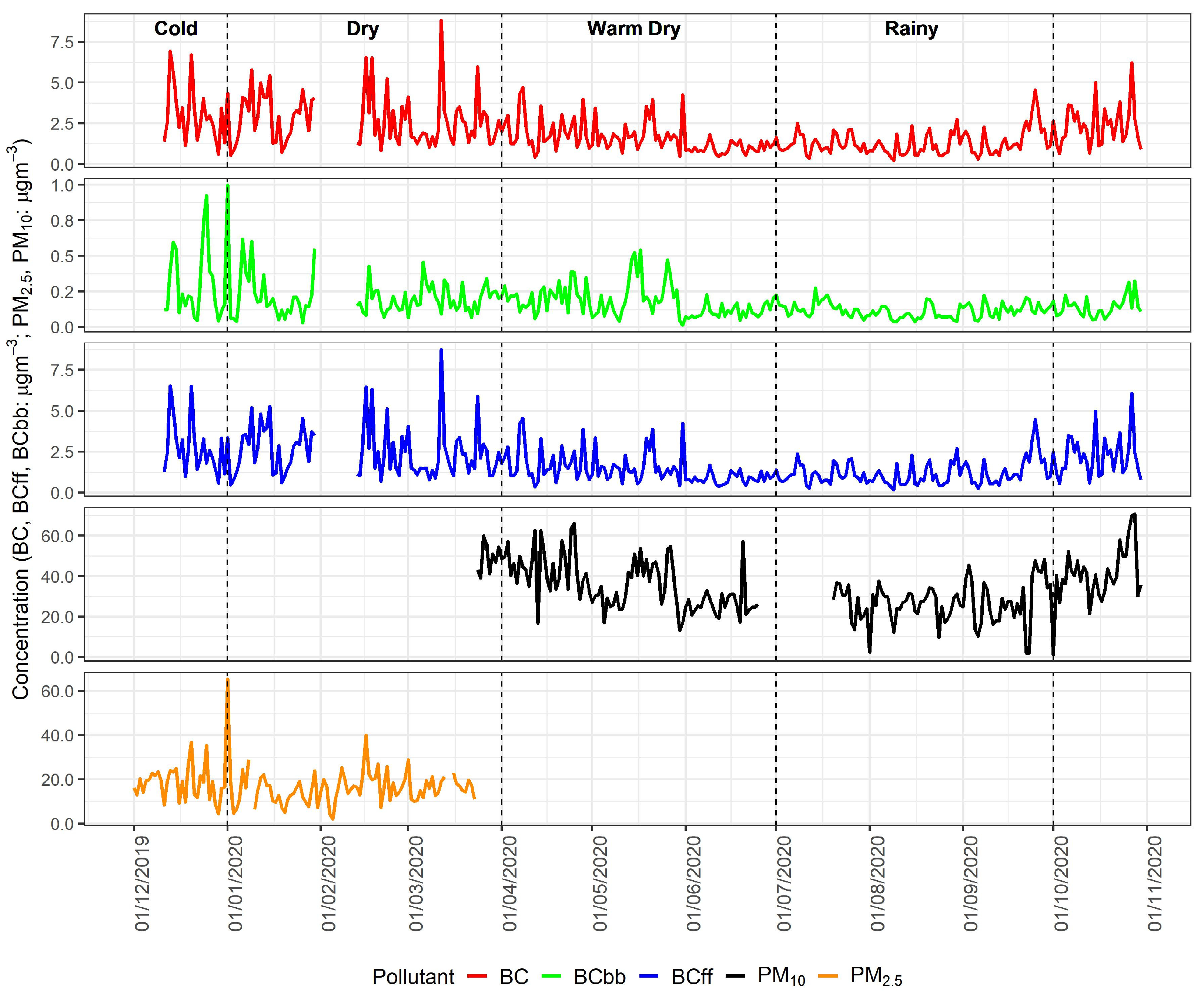
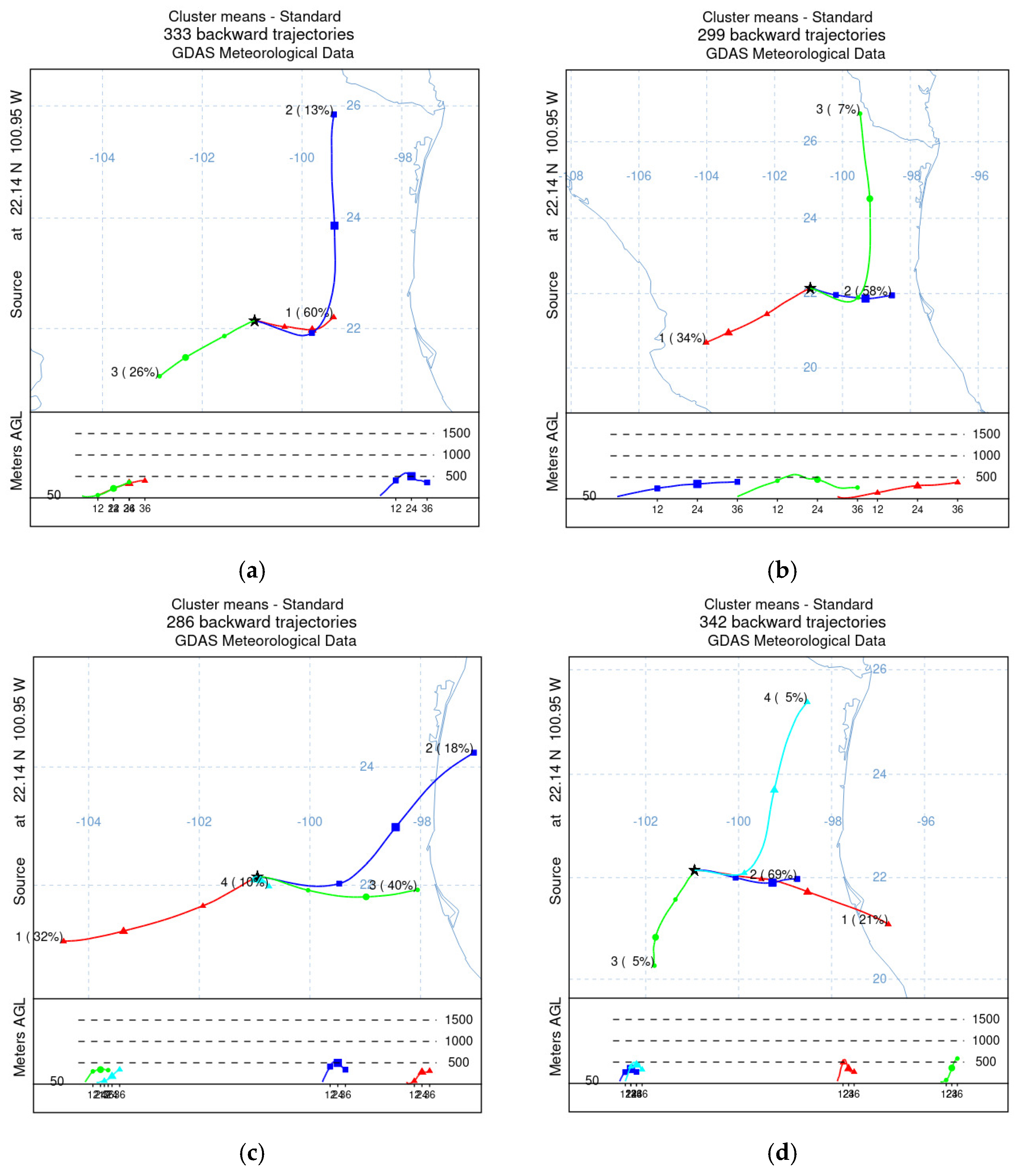
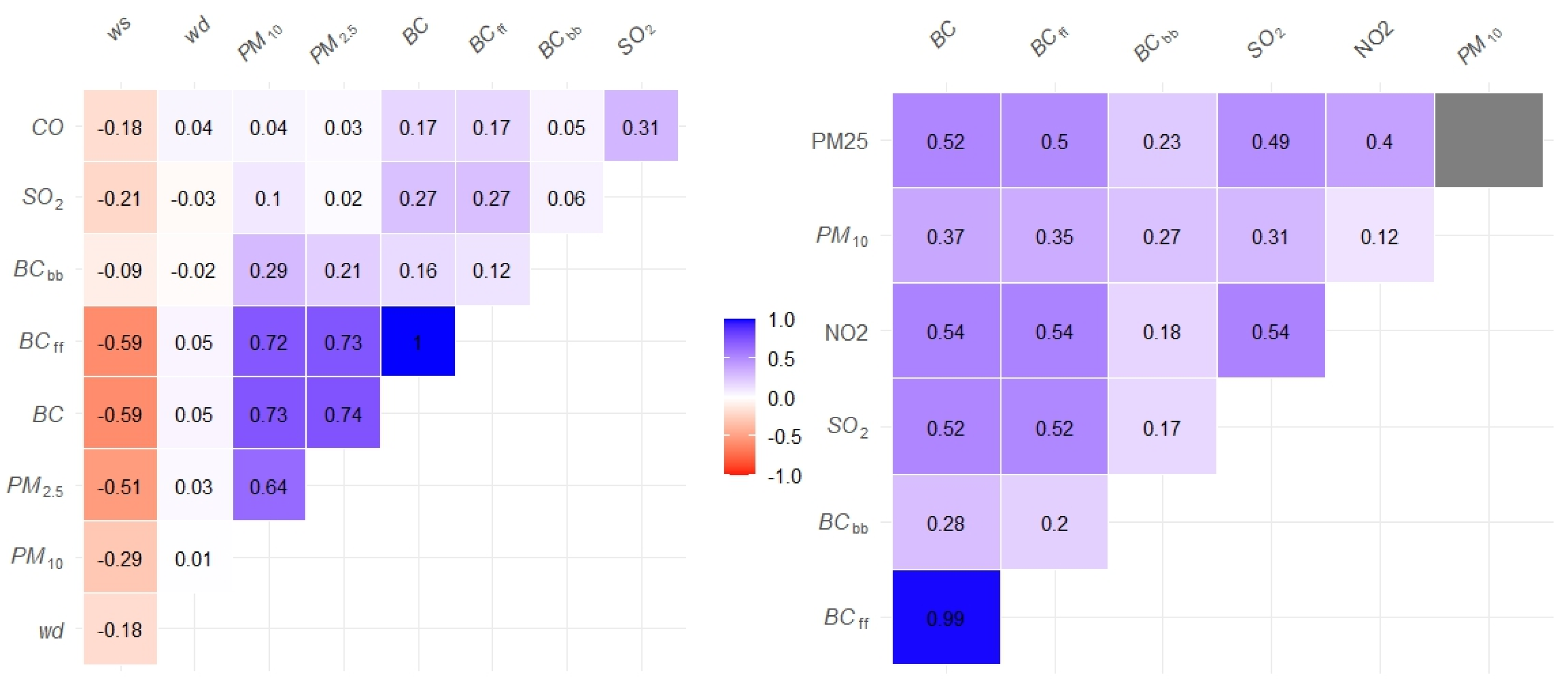
3.2. South Site Campaign at San Luis Potosi City

At this site, 315 valid samples were measured and analyzed. The annual mean concentration of BC was (1.96 µg m⁻³ with a SD of 2.54), for BCff (1.79 µg m⁻³ with a SD of 2.52 µg m⁻³) and BCbb (0.170 µg m⁻³ with a SD of 0.203 µg m⁻³). PM_2.5 concentration was (17.2 µg m⁻³ with a SD of 14.7 µg m⁻³), indicating the high variability of emissions, although it could only be measured during December and January (

Table 4. BC and other air pollutants concentrations for year 2019–2020 at South site campaign.

One Year Monitoring Campaign from December 2019 to November 2020.
	N	Mean	SD	Median	Min.	Max.	Q 0.25	Q 0.75
PM10 (µg m−3)	4785	33.8	22.7	29.0	0.001	243.0	19.0	43.0
PM2.5 (µg m−3)	2402	17.2	14.7	14.0	1.00	153.0	8.0	21.0
BC (µg m−3)	7561	1.963	2.541	1.136	0.0792	46.82	0.6768	2.079
BCbb (µg m−3)	7561	0.1700	0.2034	0.1224	0.0001	2.914	0.0608	0.2139
BCff (µg m−3)	7561	1.793	2.516	0.9627	0.0001	46.82	0.5599	1.841
SO2 (ppm)	7788	0.0023	0.0024	0.0020	0.0010	0.0780	0.0010	0.0020
NO2 (ppm)	6803	0.0130	0.0098	0.0100	0.0010	0.0770	0.0060	0.0170

). The highest PM_2.5 daily concentrations were recorded on 20, 25 and 31 December with 26.6 µg m⁻³, 35.4 µg m⁻³, and 65.5 µg m⁻³, respectively. The (BC/PM_2.5) average ratio was 0.18 a high value for medium cities but is accord, due to increased traffic due to popular festivals and fireworks and the (BCff/BC) ratio was 0.91 which is consistent with the above mentioned, however, there is a high impact for forest fires that impact in the BCbb.

On the other hand, PM₁₀ concentrations were measured for the remaining 200 days of the monitoring, where an average was (33.8 µg m⁻³ with a SD of 22.7 µg m⁻³). The highest daily concentrations were recorded on 24 and 25 April with (63.6 µg m⁻³, and 66.3 µg m⁻³, even though these two events occurred during the pandemic period; however, simultaneously some fires were recorded near the sampling point or possible fugitive emissions at night from some nearby industries [56] (Web, Mapp Firer, FIRMS, 2024).

NO₂ and SO₂ did not exceed the permissible limit values (MPL) of the NOM of the National Ministry of Health (022 and 023) [57,58] respectively during any evaluation period, which indicates that for medium-sized cities, these limits still represent very high values. Figure 6 shows the main air pollutants concentrations for this period.

Seasonally BC concentration mass data were analyzed to contrast the hypothesis of normality with the Shapiro–Wilk statistical test (α = 0.05) and the Bartlett test of homogeneity of variances test, and after concluded that all data presented a nonparametric distribution; the Mann-Whitney statistical test was used to compare the sampling years for gravimetric mass. However, all the seasons between each other presented a value (p < 0.000).

In the South zone, the cold season showed a considerably high BC concentration (2.73 µg m⁻³ with a SD of 3.27 µg m⁻³), and a relation between BCff/BC = 0.92, the cold season has a BCff/BC = 0.94, comparable to the dry season, reflecting a consistency in BC sources emission between these two seasons. The dry warm season showed a significant decrease in SO₂ and NO₂ concentration values due to the restrictive measures implemented for industries and for the general population because of the pandemic (explained later). Finally, during the rainy season, a BC decrease in the median and variability is observed, which could be indicative of a cleaner atmosphere due to the rain (

Table 5. BC and other air pollutant concentrations for seasons at South site.

	N	Mean	SD	Median	Min.	Max.	Q 0.25	Q 0.75
Dry Season. Year 2020
BC	1824	2.728	3.270	1.607	0.1087	46.82	1.054	3.079
BCbb	1824	0.2085	0.2375	0.1670	0.0001	2.833	0.0806	0.2628
BCff	1824	2.519	3.247	1.402	0.0896	46.82	0.8862	2.818
PM10	176	49.40	22.13	44.00	19.00	152.0	33.75	61.50
PM2.5	1679	16.65	14.11	13.00	1.000	153.0	8.000	21.00
SO2 (ppm)	1957	0.0030	0.0026	0.0020	0.0010	0.0330	0.0020	0.0030
NO2 (ppm)	2075	0.0166	0.0109	0.0140	0.0010	0.0610	0.0080	0.0230
Dry Warm Season. Year 2020
BC	2184	1.608	2.0467	1.010	0.190	24.72	0.6263	1.688
BCbb	2184	0.178	0.1899	0.1324	0.0001	2.284	0.0658	0.2299
BCff	2184	1.429	2.053	0.8250	0.0001	24.72	0.5118	1.423
PM10	2007	35.89	24.34	31.00	1.000	243.0	20.00	47.00
PM2.5	------	------	------	------	------	------	------	------
SO2 (ppm)	2133	0.0017	0.0009	0.0020	0.0010	0.0220	0.0010	0.0020
NO2 (ppm)	2072	0.0079	0.0052	0.0070	0.0010	0.0330	0.0040	0.0100
Rainy Season. Year 2020
BC	2208	1.285	1.534	0.7879	0.0792	21.25	0.5145	1.388
BCbb	2208	0.1162	0.0983	0.0919	0.0001	0.9278	0.0548	0.1547
BCff	2208	1.169	1.526	0.6716	0.0001	21.25	0.4249	1.224
PM10	1749	26.74	16.74	25.00	1.000	120.0	16.00	35.00
PM2.5	-----	-----	-----	-----	-----	-----	-----	-----
SO2 (ppm)	2115	0.0016	0.0009	0.0010	0.0010	0.0140	0.0010	0.0020
NO2 (ppm)	1132	0.0097	0.0056	0.0080	0.0010	0.0710	0.0060	0.0123
Cold Season. Year 2020
BC	853	2.367	3.170	1.118	0.2488	26.56	0.7172	2.550
BCbb	853	0.1363	0.1370	0.1075	0.0001	1.388	0.0555	0.1823
BCff	853	2.230	3.180	0.9694	0.2140	26.56	0.6081	2.386
PM10	853	39.98	25.08	34.00	1.000	187.0	25.00	51.00
PM2.5	----	----	----	----	----	----	----	----
SO2 (ppm)	853	0.0025	0.0043	0.0020	0.0010	0.0780	0.0010	0.0020
NO2 (ppm)	800	0.0132	0.0073	0.0110	0.0020	0.0480	0.0070	0.0180

).

Regarding the average weekly BC concentrations (Figure 7), a constant behavior is shown throughout the work week where data indicate that nearly 20% of the population travels to that area of the city; however, a small decrease can be noted for Mondays, since some freight transport rests, as well as on Saturdays and Sundays, although that area is also used for transit to go to other places outside the city as well as for recreation. However, the BC concentrations are very high despite the pandemic period. A certain value of emissions can be added to the fact that two of the largest hospitals in SLPMA are in that area and that the distribution of oxygen tanks is also in that sector of the city.

Although meteorological data were unavailable at the site, the origins of the wind directed toward the study site were determined for each of the four seasons using the HYSPLIT program (see Figure 8). Over the monitoring year, most winds originated from the east (E) with the following percentages: cold (60%), dry (58%), warm dry (40%), and rainy (69%). Additionally, a small percentage of winds came from the northeast (NE) with percentages of cold (13%), dry (7%), and rainy (5%). During the rainy season, winds also came from the southeast (SE) at 21%, and in the warm dry season, winds from the NE accounted for 18%.

Furthermore, episodes of black carbon (BC) were recorded when concentration values exceeded 5 µg/m³ for more than 5 h. A total of 47 episodes were identified, distributed as follows: 12 during the cold period, 21 during the cold dry season, 7 during the hot dry season, and 7 during the rainy season. The main origins of these episodes were identified: 15 events originated from the northwest (NW), where the downtown area of the city, a PEMEX plant, and several newly established brickyards are located. Additionally, 12 episodes came from the NE, including the brick-making area and some industrial cement and foundry plants. Nine episodes were traced back to the E, where Highway 70 runs, an area with heavy freight vehicle traffic and numerous illegal garbage burnings. Lastly, 9 emissions were recorded from the south, coinciding with the San Luis Potosí industrial zone.

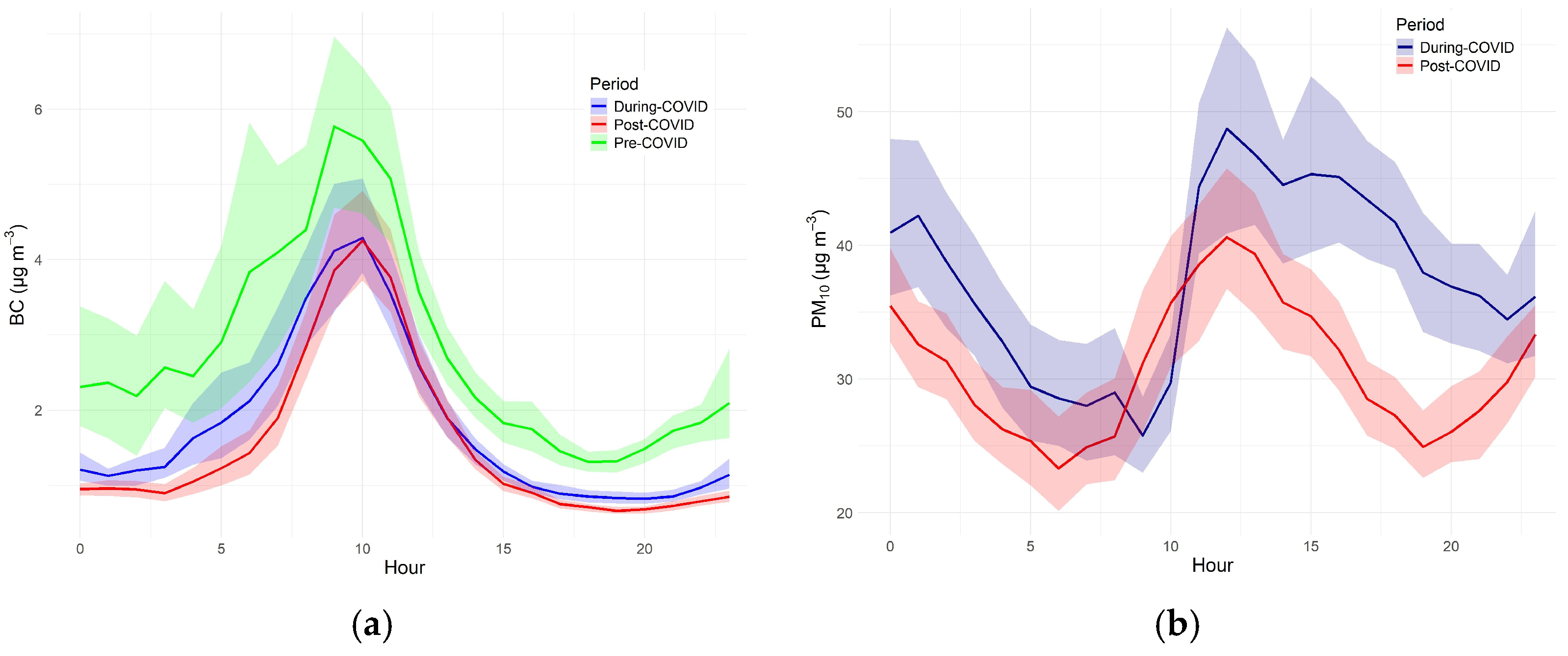
3.3. BC Concentration Analysis During the Contingency SARS-CoV-2 Period

On the other hand, in 2020, the health contingency situation due to the SARS-CoV-2 virus modified all the emission sources in the city.

Due to the different health actions regulated by each state and by the federal government during the contingency phase, many private and federal vehicles stopped circulating, industrial activities decreased their production, and, in certain weeks, were suspended, which led to changes in emissions in the study area. Furthermore, monitoring systems in the city were neglected; however, a few of the automatic sampling equipment continued to generate data. This was the case with the BC aethalometer equipment. For this reason, this evaluation was carried out considering emissions according to the phase of the pandemic, and three different stages to evaluate this period and divided into pre-contingency of COVID from November 2019 to 20 March 2020, the second period named Contingency of COVID from 21 March to 27 June, and a post-contingency period from 28 June to November 2020 (

Table 6. Air pollutants concentrations for the contingency evaluation period.

Season	BC (μg m−3)	BCff (μg m−3)	BCbb (μg m−3)	PM10 (μg m−3)	PM2.5 (μg m−3)	SO2 (ppm)	NO2 (ppm)
Pre-COVID-2	2.853 ± 0.0712	2.623 ± 0.0700	0.2300 ± 0.0065	---------	17.07 ± 0.3304	0.0033 ± 0.0001	0.0180 ± 0.0002
COVID Contingency	1.709 ± 0.0440	1.528 ± 0.0442	0.1810 ± 0.0038	36.98 ± 0.5231	17.53 ± 1.146	0.0018 ± 0.0001	0.0082 ± 0.0001
Post-COVID-2	1.5774 ± 0.0385	1.455 ± 0.0385	0.1229 ± 0.0020	31.08 ± 0.4079	---------	0.0018 ± 0.0001	0.0111 ± 0.0001

).

The nonparametric Kruskal-Wallis test was used to assess overall variations between the pre-COVID, during COVID, and post-COVID periods, followed by Dunn’s post-hoc test with Bonferroni correction to identify significant differences between pairs (p < 0.05). These tests were selected because the data did not meet the assumptions of normality or homogeneity of variances. The statistical analyses confirmed that all pairwise comparisons between periods were highly significant (p < 0.001).

The calculated statistics reveal interesting trends in BC concentrations and other air pollutants. Before the contingency (pre-COVID), the average BC concentrations were significantly higher (2.85 ± 0.071 µg/m³) compared to the periods during and after the contingency, with 1.71 ± 0.044 µg/m³ and 1.58 ± 0.038 µg/m³, respectively. This notable reduction during and after the contingency (Kruskal-Wallis χ² = 1064.6, df = 2) suggests decreased pollutant emissions due to mobility restrictions and reduced industrial and vehicular activity.

Regarding Black Carbon fractions, both the fraction from fossil fuels (BCff) and biomass (BCbb) followed a similar trend, decreasing during and after the contingency. For BCff, concentrations dropped in pre-COVID from 2.62 ± 0.700 µg/m³ to 1.53 ± 0.044 µg/m³ during COVID and 1.45 ± 0.038 µg/m³ in post-COVID period. For BCbb, reductions were also observed, although less pronounced, indicating that emissions from biomass were less affected and produced during these periods.

The analysis of PM₁₀ and PM_2.5 is also revealing. Although no PM₁₀ data were available for the pre-COVID period, just during and after the contingency, the recorded PM₁₀ levels were 36.9 ± 0.523 µgm⁻³ and 31.1 ± 0.408 µgm⁻³, respectively, which may reflect changes in local activities that generate suspended particles. (Figure 9). Daily BC average concentrations showed higher concentrations during the pre-COVID period, due to increased traffic in the area and common industrial activities in addition to lower winds that caused less dispersion of the pollutants. In the case of PM₁₀, during the COVID period, despite the reduction in industrial activity and the decrease in vehicles circulating in the area, particle increases were observed during the hours with greater photochemical activity, which indicates the formation of secondary particles. This was verified by employing the Ozone data column concentrations obtained from the SENTINEL-5P satellite for the year 2020, which showed higher concentrations from May to July.

PM_2.5 levels decreased slightly from 17.1 ± 0.330 µg/m³ in the pre-COVID period to 17.5 ± 1.15 µg/m³ during the contingency, which could be attributed to a combination of factors, including changes in emission sources and meteorological conditions like high temperatures and radiation values, and the subsequence increase in ozone concentrations during Spring and Summer when COVID contingency period occurred, that could produce secondary reactions between gases as COVs with other precursors of particulate matter.

SO₂ and NO₂ levels also decreased during the contingency, which could be related to a reduction in industrial activities and vehicular traffic. These findings highlight the direct impact of human activities on urban air quality and the importance of environmental management policies in mitigating air pollution.

4. Discussion

Due to the non-parametric distribution of air pollutant data, it was necessary to find a more robust method against extreme values and asymmetric distributions. Figure 10 represents a correlation matrix plot (Spearman correlations) between the air pollutants and wind speed (ws) and wind direction (wd) for all the evaluation periods at each monitoring site. The intensity or blue color indicates a positive correlation, which represents the strength of the relationship between each pair of parameters.

Moreover, Figure 10 showed the highest correlations (r > 0.99), for BC and BCff which indicated that their emission was majorly emitted for the same process in both monitoring zones.

At the North site, a significant correlation between BC and PM can be observed (r > 0.73). A conversely weak positive correlation between CO and SO₂ (r = 0.31), for all the period and the correlation analysis between BC and PMs with meteorological conditions indicated high negative correlations (r < −0.51), with wind speed, which indicated that ws low values were associated with high concentrations of all the types of particles, especially BC and BCff. The polar coordinate system showed only high concentrations of BCff near the sampling site, confirming this association.

Hourly PM₁₀ concentration values were recorded at elevated levels (>100 µg m⁻³) on at least 38 days, with most of these instances lasting more than 3 h. However, only on nearly 10 days the concentrations exceeded the National Official Mexican Standard (NOM) for health risk in effect that year [59]. These high concentration emissions can be categorized as “episodes”: on 3 of these days, the levels exceeded 200 µg m⁻³, on 5 days the concentrations ranged from 150 µg m⁻³ to 200 µg m⁻³, and on 22 days, the concentrations were between 100 µg m⁻³ and 150 µg m⁻³. Notably, only 11 episodes lasted more than 6 continuous hours at these elevated levels.

High emissions often result from point sources such as brick kilns, ceramic kilns, or forest fires, which can produce significant concentrations in less than 12 h. This is emphasized by regulatory standards aimed at prompting actions to alert and protect the local population. Additionally, black carbon (BC) emissions were higher than 2 µg m⁻³ in 87% of these episodes, highlighting the link between incomplete combustion and PM₁₀ emissions in the area. This suggests a potential need to regulate or adjust the health risk standards to shorter periods, particularly for medium-sized cities, to facilitate more timely and effective responses. In addition, 75% of these episodes of air pollution, their origin or emission correspond to the area where the brick kilns are located, which indicates the need to take actions to regulate fuels and/or relocate them to areas outside the city where their emissions have no impact on it. It should be noted that reducing emissions from the brick zone would significantly reduce the concentrations of PMs and BC within the city of SLP.

At the south site, a relative correlation of BC with SO₂ and NO₂ (r > 0.52) could be observed, which showed the emission of these pollutants from fixed sources such as industries in that area, that remained working during the COVID-19 period. In the same way, SO₂ and NO₂ also show a relative correlation (r = 0.54) for this sampling year.

Furthermore, during the COVID-19 period, it was remarkable that despite the reduction of vehicular sources by almost 50%, emissions from the industrial sector remained constant. Together with the high photochemical reactivity characteristic of the hot period, this promoted the formation of atmospheric particles at levels like in previous years.

The average annual concentration of Black Carbon (BC) in San Luis Potosí (SLP) ranged between 1.11 µg m⁻³ at the northern site and 1.96 µg m⁻³ at the southern site. These values are lower than those reported from high urban cities like Mexico City during 2013–2014, where Retama et al. (2015) observed daily averages of 8.8 µg m⁻³ during the rainy season and 13.1 µg m⁻³ in the dry season. Similarly, in Guadalajara, Limon-Sanchez et al. (2011) reported BC levels during the dry season ranging between (1.3–8.7) µg m⁻³ at the “Centro” monitoring site, and between (1.5–13.8) µg m⁻³ at the Miravalle site. In comparison, BC concentrations in growing urban areas in 2019, such as Monterrey (2.5 µg m⁻³) and Juriquilla (0.75 µg m⁻³), according to Peralta et al., were closer to those observed in SLP. These differences highlight the influence of local sources and meteorological conditions on BC levels, with urban and industrial zones experiencing significantly higher concentrations than suburban areas in Mexican cities [60,61,62].

Additionally, combustion processes and traffic-related emissions have been linked as the main primary particulate matter sources noticed in other urban areas [62,63]. It has been demonstrated that black carbon (BC) is a significant type of particulate matter emitted from the combustion of fossil fuels, particularly in relation to vehicle emissions, with a notable connection to heavy-duty diesel vehicles [64,65]. Additionally, when examining the emission characteristics of fossil fuel combustion—termed BCff—it’s observed that more complete combustion results in lower emissions of carbon monoxide (CO), particulate matter (PMs), and organic compounds for each unit of fuel burned. However, this process generates higher levels of nitrogen oxides (NO_X) compared to black carbon from biomass burning (BCbb), which can be attributed to the elevated combustion temperatures and the presence of excess air [66].

Toxicological studies in the SLPMA suggested that fossil fuel and biomass combustion processes can significantly contribute to adverse health outcomes [67,68], especially due to the large contribution of other associated air pollutants with these processes, such as PAHs, CO, dioxins, BTEX and other organic compounds that have been evaluated in the brick kiln areas of SLP and mainly in various exposure markers in workers [69,70,71]. The episodes of high PM concentration measured in the city of SLP represent a high risk to the health of the population due to acute toxicity and exposure to chronic toxicity and can cause high healthcare costs.

BC emissions from open-air fires and waste were recently included in emissions inventories used to model and develop local and national climate change mitigation policies. BC concentration measurements also represent a good indicator to assess these emissions and to generate more accurate factor emissions for different regions.

The rapid growth of urbanization and transport demand in medium-sized cities in Mexico and other countries has increased air pollution and GHG emissions and will pose a major challenge for developing countries in the next few years.

5. Conclusions

Due to the many emission sources generated in its extension, the SLPMA represents an area of great interest for studying air pollution. This work evaluated the air pollution generated mainly as BC and other associated pollutants. It was possible to observe different magnitudes of concentrations and periods of emission times present in the two study areas and demonstrate the different seasonal patterns.

On the one hand, in the northern site, there were daily concentrations (Annual average BC = 1.11 µg m⁻³) that can be considered low. However, in this area, there are also very high levels of continuous emissions during certain intervals of the day between 5 h and 12 h generated by specific fixed sources that can contribute to respiratory, cardiovascular, or reproductive diseases, mainly at a chronic level for the population of the area.

While in the southern site (annual average BC = 1.96 µg m⁻³), concentrations were higher than in the other study site, even though the global COVID-19 pandemic occurred and in certain months of the year, the mobile sources present in this area of high vehicular traffic decreased considerably. The freight vehicles in this area may be the main cause of these high emissions. These emissions may cause illnesses due to high levels of exposure compared to other Mexican cities [54,61,62], even more so for the population that lives there or regularly works there. It would be advisable to carry out another study in the same area or a site closer to the industrial zone to better understand its impacts.

It is important to evaluate black carbon due to its effects on the health of the human population, local air pollution, and global climate change. These characteristics promote it as a new indicator of air quality worldwide. However, in Mexico, this pollutant has not yet been evaluated in many of the large, medium-sized, or growing cities, and it is necessary to know the dynamics of the emissions generated by the various sources of incomplete combustion and even more so since, as is the case in San Luis Potosí city, because distinct sources generate the emissions. It is important to evaluate both fixed and mobile sources in different zones of the cities to develop appropriate reduction and mitigation strategies for specific cities in the country.

PM concentration values are generally lower than the official 24-h average standards determined by the NOM; however, it is necessary to delve deeper into their composition. BC represents a new indicator for evaluating incomplete combustion processes, especially in cities. In this study, it was possible to estimate the daily, weekly, and seasonal patterns, as well as their associations with the prevailing winds for two sites in the city of San Luis Potosí. It was also possible to determine the average daily and annual BC concentrations, as well as the main emission sources, and correlations they have with other pollutants from incomplete combustion such as BCff, and CO. They can serve as comparisons for other cities, with similar characteristics and especially for medium-sized Mexican cities that do not yet have BC assessments.

This work provides valuable information that may be useful worldwide for calibrating satellite observations through ground-level measurements. Finally, an assessment of BC and other air pollutants that could be measured and evaluated based on the different stages during the SARX COVID-19 pandemic, which occurred in 2020, was performed and showed no significant variation in the concentration from air pollutants from recent two years.

References

1. WHO: World Health Organization. Fact Sheet N 313. 2 May 2018. Available online: https://www.who.int/news-room/fact-sheets/detail/ambient-(outdoor)-air-quality-and-health (accessed on 14 August 2022).
2. WHO: World Health Organization. WHO global air quality guidelines. Coast. Estuar. Process. 2021. Available online: https://www.who.int/publications/i/item/9789240034228 (accessed on 31 December 2024).
3. WHO: World Health Organization. Health Effects of Particulate Matter. Policy Implications for Countries in Eastern Europe, Caucasus and Central ASIA. 2013. Regional Office for Europe. Available online: https://apps.who.int/iris/handle/10665/344854 (accessed on 21 August 2022).
4. Aiken, A.C.; De Foy, B.; Wiedinmyer, C.; Decarlo, P.F.; Ulbrich, I.M.; Wehrli, M.N.; Jimenez, J.L. Mexico City aerosol analysis during MILAGRO using high resolution aerosol mass spectrometry at the urban supersite (T0)-Part 2: Analysis of the biomass burning contribution and the nonfossil carbon fraction. Atmos. Chem. Phys. 2010, 12, 5315–5341. [Google Scholar] [CrossRef]
5. Kirchstetter, T.W.; Thatcher, T.L. Contribution of organic carbon to wood smoke particulate matter absorption of solar radiation. Atmos. Chem. Phys. 2012, 12, 6067–6072. [Google Scholar] [CrossRef]
6. Solís, C.; Gómez, V.; Ortíz, E.; Chávez, E.; Miranda, J.; Aragón, J.; Martínez, M.A.; Castro, T.; Peralta, O. AMS 14C and chemical composition of atmospheric aerosols from Mexico City. Radiocarbon 2017, 59, 321–332. [Google Scholar] [CrossRef]
7. Bond, T.C.; Dhoerty, S.J.; Fahey, D.W.; Forster, P.M.; Berntsen, T.; DeAngelo, B.J.; Flanner, M.G.; Ghan, S.; Kärcher, B.; Koch, D.; et al. Bounding the role of black carbon in the climate system: A scientific assesment. J. Geophys. Res. 2013, 118, 5380–5552. [Google Scholar] [CrossRef]
8. Croft, B.; Lohmann, U.; Salzen, K.V. Black carbon ageing in the canadian centre for climate modelling and analysis atmospheric general circulation model. Atmos. Chem. Phys. Discuss. 2005, 5, 1931–1949. [Google Scholar] [CrossRef]
9. Lack, D.A.; Moosmüller, H.; McMeeking, G.R.; Chakrabarty, R.K.; Baumgardner, D. Characterizing elemental, equivalent black, and refractory black carbon aerosol particles: A review of techniques, their limitations and uncertainties. Anal. Bioanal. Chem. 2014, 406, 99–122. [Google Scholar] [CrossRef] [PubMed]
10. Yao, L.; Yang, L.; Chen, J.; Wang, X.; Xue, L.; Li, W.; Sui, X.; Wen, L.; Chi, J.; Zhu, Y.; et al. Characteristics of carbonaceous aerosols: Impact of biomass burning and secondary formation in summertime in a rural area of the North China Plain. Sci. Total Environ. 2016, 557–558, 520–530. [Google Scholar] [CrossRef] [PubMed]
11. Wang, R.; Balkanski, Y.; Boucher, O.; Ciais, P.; Schuster, G.L.; Chevallier, F.; Samset, B.H.; Liu, J.; Piao, S.; Valari, M.; et al. Estimation of global black carbon direct radiative forcing and its uncertainty constrained by observations. J. Geophys. Res. Atmos. 2016, 121, 5948–5971. [Google Scholar] [CrossRef]
12. Watson, J.G. Visibility: Science and Regulation. J. Air Waste Manag. Assoc. 2002, 52, 628–713. [Google Scholar] [CrossRef] [PubMed]
13. Wang, Q.; Schwarz, J.P.; Cao, J.; Gao, R.; Fahey, D.W.; Hu, T.; Huang, R.J.; Han, Y.; Shen, Z. Black carbon aerosol characterization in a remote area of Qinghai–Tibetan Plateau, western China. Sci. Total Environ. 2014, 479–480, 151–158. [Google Scholar] [CrossRef] [PubMed]
14. Auffhammer, M.; Ramanathan, V.; Vincent, J.R. Integrated model shows that atmospheric brown clouds and greenhouse gases have reduced rice harvests in India. Proc. Natl. Acad. Sci. USA 2006, 103, 19668–19672. [Google Scholar] [CrossRef] [PubMed]
15. UNEP. United Nations Environment Programme. An Assessment of Emissions and Mitigation Options for Black Carbon for the Arctic Council; Technical Report of the Arctic Council Task Force on ShortLived Climate Forcers 2011. Available online: https://www.unep.org/resources/report/assessment-emissions-and-mitigation-options-black-carbon-arctic-counciltechnical (accessed on 14 August 2022).
16. Tomlin, A.S. Air Quality and Climate Impacts of Biomass Use as an Energy Source: A Review. Energy Fuels 2021, 35, 14213–14240. [Google Scholar] [CrossRef]
17. Straif, K.; Cohen, A.; Samet, J. Air Pollution and Cancer. International Agency for Research on Cancer; IARC Scientific Publications: Lyon, France, 2013; p. 161. ISBN 978-92-832-2166-1/0300-5085. [Google Scholar]
18. Schraufnagel, D.E.; Balmes, J.R.; Cowl, C.T.; De Matteis, S.; Jung, S.-H.; Mortimer, K.; Perez-Padilla, R.; Rice, M.B.; Riojas-Rodriguez, H.; Sood, A.; et al. Air Pollution and Noncommunicable Diseases. A Review by the Forum of International Respiratory Societies’ Environmental Committee, Part 1: The Damaging Effects of Air Pollution. Chest 2019, 155, 409–416. [Google Scholar] [CrossRef] [PubMed]
19. Schraufnagel, D.E.; Balmes, J.R.; Cowl, C.T.; De Matteis, S.; Jung, S.-H.; Mortimer, K.; Perez-Padilla, R.; Rice, M.B.; Riojas-Rodriguez, H.; Sood, A.; et al. Air Pollution and Noncommunicable Diseases. A Review by the Forum of International Respiratory Societies’ Environmental Committee, Part 2: Air Pollution and Organ Systems. Chest 2019, 155, 417–426. [Google Scholar] [CrossRef]
20. Hoffmann, B.; Moebus, S.; Dragano, N.; Stang, A.; Möhlenkamp, S.; Schmermund, A.; Memmesheimer, M.; Bröcker-Preuss, M.; Mann, K.; Erbel, R.; et al. Chronic Residential Exposure to Particulate Matter Air Pollution and Systemic Inflammatory Markers. Environ. Health Perspect. 2009, 117, 1302–1308. [Google Scholar] [CrossRef]
21. Wyzga, R.E.; Rohr, A.C. Long-term particulate matter exposure: Attributing health effects to individual PM components. J. Air Waste Manag. Assoc. 2015, 65, 523–543. [Google Scholar] [CrossRef] [PubMed]
22. Michael, S.; Montag, M.; Dott, W. Pro-inflammatory effects and oxidative stress in lung macrophages and epithelial cells induced by ambient particulate matter. Environ. Pollut. 2013, 183, 19–89. [Google Scholar] [CrossRef]
23. Lippmann, M.; Chen, L.-C. Health effects of concentrated ambient air particulate matter (CAPs) and its components. Crit. Rev. Toxicol. 2009, 39, 865–913. [Google Scholar] [CrossRef] [PubMed]
24. Knaapen, A.M.; Borm, P.J.; Albrecht, C.; Schins, R.P. Inhaled particles and lung cancer. Part A: Mechanisms. Int. J. Cancer 2004, 109, 799–809. [Google Scholar] [CrossRef] [PubMed]
25. Aslam, I.; Roeffaers, M.B.J. Carbonaceous Nanoparticle Air Pollution: Toxicity and Detection in Biological Samples. Nanomaterials 2022, 12, 3948. [Google Scholar] [CrossRef]
26. Karanasiou, A.; Alastuey, A.; Amato, F.; Renzi, M.; Stafoggia, M.; Tobias, A.; Reche, C.; Forastiere, F.; Gumy, S.; Mudu, P.; et al. Short-term health effects from outdoor exposure to biomass burning emissions: A review. Sci. Total Environ. 2021, 781, 146739. [Google Scholar] [CrossRef] [PubMed]
27. Yang, Y.; Ruan, Z.; Wang, X.; Yang, Y.; Mason, T.G.; Lin, H.; Tian, L. Shortterm and long-term exposures to fine particulate matter constituents and health: A systematic review and meta-analysis. Environ. Pollut. 2019, 247, 874–882. [Google Scholar] [CrossRef]
28. Pope, C.A., III; Dockery, D.W. Health Effects of Fine Particulate Air Pollution: Lines that Connect. J. Air Waste Manag. Assoc. 2006, 56, 709–742. [Google Scholar] [CrossRef]
29. Pacyna, J.M.; Breivik, K.; Münch, J.; Fudala, J. European atmospheric emissions of selected persistent organic pollutants, 1970–1995. Atmos. Environ. 2003, 37, S119–S131. [Google Scholar] [CrossRef]
30. Janssen, N.A.H.; Hoek, G.; Simic-Lawson, M.; Fischer, P.; van Bree, L.; Ten Brink, H.; Keuken, M.; Atkinson, R.W.; Anderson, H.R.; Brunekreef, B.; et al. Black Carbon as an Additional Indicator of the Adverse Health Effects of Airborne Particles Compared with PM10 and PM2.5. Environ. Health Perspect. 2011, 119, 1691–1699. [Google Scholar] [CrossRef] [PubMed]
31. Petzold, A.; Ogren, J.A.; Fiebig, M.; Laj, P.; Li, S.-M.; Baltensperger, U.; Holzer-Popp, T.; Kinne, S.; Pappalardo, G.; Sugimoto, N.; et al. Recommendations for reporting “black carbon” measurements. Atmos. Chem. Phys. 2013, 13, 8365–8379. [Google Scholar] [CrossRef]
32. Mousavi, A.; Sowlat, M.H.; Hasheminassab, S.; Polidori, A.; Sioutas, C. Spatio-temporal trends and source apportionment of fossil fuel and biomass burning black carbon (BC) in the Los Angeles Basin. Sci. Total Environ. 2018, 640–641, 1231–1240. [Google Scholar] [CrossRef] [PubMed]
33. Birmili, W.; Achtert, P.; Nowak, A.; Wehner, B.; Wiedensohler, A.; Takegawa, N.; Kondo, Y.; Miyazaki, Y.; Hu, M.; Zhu, T. Hygroscopic growth of tropospheric particle number size distributions over the North China Plain. J. Geophys. Res. 2009, 114, D00G07. [Google Scholar] [CrossRef]
34. Kondo, Y.; Komazaki, Y.; Miyazaki, Y.; Moteki, N.; Takegawa, N.; Kodarna, D.; Deguchi, S.; Nogarni, M.; Fukuda, M.; Miyakawa, T.; et al. Temporal variations of elemental carbon in Tokyo. J. Geophys. Res. Atmos. 2006, 111, D12205. [Google Scholar] [CrossRef]
35. Yang, F.; He, K.; Ye, B.; Chen, K.; Cha, L.; Cadle, S.H.; Chan, T.; Mulawa, P.A. One-year record of organic and elemental carbon in fine particles in downtown Beijing and Shanghai. Eur. Geosci. Union 2005, 5, 1449–1457. [Google Scholar] [CrossRef]
36. Instituto Nacional de Ecologia y Cambio Climatico (INECC). Inventario Nacional de Emisiones de Gases y Compuestos de Efecto Invernadero 1990–2015, Resumen Informativo, Ciudad de México. 2018. Available online: https://datos.gob.mx/busca/dataset/inventario-nacional-de-emisiones-de-gases-y-compuestos-de-efecto-invernadero-inegycei (accessed on 31 December 2024).
37. Aragón, P.A.; Campos, R.A.; Leyva, R.R.; Hernández, O.M.; Miranda, O.N.; Luszczewski-Kudra, A. Influencia de emisiones industriales en el polvo atmosférico de la ciudad de San Luis Potosí, México. Rev. Int. Contam. Ambient. 2006, 22, 1. [Google Scholar]
38. Barrera, V.; Contreras, C.; Mugica-Alvarez, V.; Galindo, G.; Flores, R.; Miranda, J. PM2.5. Characterization and Source Apportionment using Positive Matrix Factorization at San Luis Potosi City, Mexico, during the years 2017–2018. Atmosphere 2023, 14, 1160. [Google Scholar] [CrossRef]
39. Aragón, P.A.; Torres, V.G.; Santiago, J.P.; Monroy, F.M. Scanning and transmission electron microscope of suspended lead-rich particles in the air of San Luis Potosi, Mexico. Atmos. Environ. 2002, 36, 5235–5243. [Google Scholar] [CrossRef]
40. Aragón, P.A.; Torres, V.G.; Monroy, F.M.; Luszczewski, K.A.; Leyva, R.R. Scanning electron microscope and statistical analysis of suspended heavy metal particles in San Luis Potosi, Mexico. Atmos. Environ. 2000, 34, 4103–4112. [Google Scholar] [CrossRef]
41. Pineda, L.M.; Carbajal, N.; Campos, R.A.; Aragón, P.A.; García, A.R. Dispersion of atmospheric coarse particulate matter in the San Luis Potosí, Mexico, urban area. Atmósfera 2014, 27, 5–19. [Google Scholar] [CrossRef]
42. SCT: Secretaria de Comunicaciones y Transporte. Infraestructura Dirección General de Servicios Técnicos. Datos Viales 2024. Available online: https://www.sct.gob.mx/fileadmin/DireccionesGrales/DGST/Datos_Viales_2024/24_SLP_DV2024.pdf (accessed on 21 November 2024).
43. SEGAM: Secretaria de Ecología y Gestión Ambiental. Inventario de Emisiones a la Atmósfera Estado de San Luis Potosí, México. Reporte Final (2013). Available online: https://slp.gob.mx/segam/Documentos%20compartidos/ESTUDIOS%20PROGRAMAS%20Y%20PROYECTOS/InventarioEstataldeEmisiones_SLP-2011.pdf (accessed on 26 November 2024).
44. INEGI: Instituto Nacional de Estadística y Geografía. Encuesta Intercensal 2015: Marco conceptual/INEGI, México. 2018. Available online: https://www.inegi.org.mx/rnm/index.php/catalog/214 (accessed on 13 December 2024).
45. Hansen, A.D.A.; Rosen, H.; Novakov, T. The aethalometer—An instrument for the real-time measurement of optical absorption by aerosol particles. Sci. Total Environ. 1984, 36, 191–196. [Google Scholar] [CrossRef]
46. Drinovec, L.; Močnik, G.; Zotter, P.; Prévôt, A.S.H.; Ruckstuhl, C.; Coz, E.; Rupakheti, M.; Sciare, J.; Müller, T.; Wiedensohler, A.; et al. The “dual-spot” Aethalometer: An improved measurement of aerosol black carbon with real-time loading compensation. Atmos. Meas. Tech. 2015, 8, 1965–1979. [Google Scholar] [CrossRef]
47. SEMARNAT: Secretaría de Medio Ambiente y Recursos Naturales. SINAICA. National Monitoring Network Datasets. 2021. Available online: http://sinaica.ine.gob.mx/ (accessed on 25 June 2021).
48. Méndez Espinosa, J.F.; Pinto Herrera, L.C.; Galvis Remolina, B.R.; Pachón, J.E. Estimación de factores de emisión de material particulado resuspendido antes, durante y después de la pavimentación de una vía en Bogotá. Cienc. Ing. Neogranadina 2017, 27, 43–60. [Google Scholar] [CrossRef]
49. Draxler, R.R.; Rolph, G.D. HYSPLIT (HYbrid Single-Particle Lagrangian Integrated Trajectory) Model access via NOAA ARL READY Website 2010. Available online: https://ready.arl.noaa.gov/HYSPLIT.php (accessed on 11 December 2024).
50. Carslaw, D.C.; Ropkins, K. Openair—An R package for air quality data analysis. Environ. Model. Softw. 2012, 27–28, 52–61. [Google Scholar] [CrossRef]
51. Clarke, K.C. Advances in geographic information systems, computers. Environ. Urban Syst. 1986, 10, 175–184. [Google Scholar] [CrossRef]
52. NOM-025-SSA1-2014; SSA: Secretaria de Salud. Mexican Official Standard, Permissible Limits for PM10 and PM2.5 Suspended Particle Concentrations in Air and Evaluation Criteria. Diario Oficial de la Federación: Mexico City, Mexico, 2014.
53. Thamban, N.M.; Tripathi, S.N.; Moosakutty, S.P.; Kuntamukkala, P.; Kanawade, V.P. Internally mixed black carbon in the Indo-Gangetic Plain and its effect on absorption enhancement. Atmos. Res. 2017, 197, 211–223. [Google Scholar] [CrossRef]
54. Leyte-Lugo, M.; Sandoval, B.; Salcedo, D.; Peralta, O.; Castro, T.; Alvarez-Ospina, H. Variations of Black Carbon Concentrations in Two Sites in Mexico: A High-Altitude National Park and a Semi-Urban Site. Atmosphere 2022, 13, 216. [Google Scholar] [CrossRef]
55. Enroth, J.; Saarikoski, S.; Niemi, J.; Kousa, A.; Ježek, I.; Močnik, G.; Carbone, S.; Kuuluvainen, H.; Rönkkö, T.; Hillamo, R.; et al. Chemical and physical characterization of traffic particles in four different highway environments in the Helsinki metropolitan area, Atmos. Chem. Phys. 2016, 16, 5497–5512. [Google Scholar] [CrossRef]
56. NASA-FIRMS. Fire Information for Resource Management System. Available online: https://firms.modaps.eosdis.nasa.gov/map (accessed on 21 August 2021).
57. NOM-022-SSA1-2019; SSA: Secretaría de Salud. Mexican Official Standard, Criteria for Evaluating Ambient Air Quality with Respect to Sulfur Dioxide (SO2). Standard Values for the Concentration of Sulfur Dioxide (SO2) in Ambient Air, as a Measure to Protect the Health of the Population. Diario Oficial de la Federación: Mexico City, Mexico, 2019.
58. NOM-023-SSA1-2021; SSA: Secretaría de Salud. Mexican Official Standard, Environmental Health. Criteria for Evaluating Ambient Air Quality with Respect to Nitrogen Dioxide (NO2). Standard Values for the Concentration of Nitrogen Dioxide (NO2) in Ambient Air, as a Measure to Protect the Health of the Population. Diario Oficial de la Federación: Mexico City, Mexico, 2021.
59. NOM-172-SEMARNAT-2019; SEMARNAT: Secretaría de Medio Ambiente y Recursos Naturales. Norma Oficial Mexicana, Lineamientos Para la Obtención y Comunicación del Índice de Calidad del Aire y Riesgos a la Salud. Diario Oficial de la Federación: Ciudad de Mexico, Mexico, 2019.
60. Retama, A.; Baumgardner, D.; Raga, G.B.; McMeeking, G.R.; Walker, J.W. Seasonal and diurnal trends in black carbon properties and co-pollutants in Mexico City. Atmos. Chem. Phys. 2015, 15, 9693–9709. [Google Scholar] [CrossRef]
61. Limon, M.T.; Carbajal, R.P.; Hernandez, M.L.; Saldarriaga, N.H.; Lopez, L.A.; Cosio, R.R.; Arriaga, C.J.; Smith, W. Black carbon in PM2.5, data from two urban sites in Guadalajara, Mexico during 2008. Atmos. Pollut. Res. 2008, 2, 358–365. [Google Scholar] [CrossRef]
62. Peralta, O.; Ortínez-Alvarez, A.; Basaldud, R.; Santiago, N.; Alvarez-Ospina, H.; De la Cruz, K.; Barrera, V.; De la Luz Espinosa, M.; Saavedra, I.; Castro, T.; et al. Atmospheric black carbon concentrations in Mexico. Atmos. Res. 2019, 230, 104626. [Google Scholar] [CrossRef]
63. Squizzato, S.; Cazzaro, M.; Innocente, E.; Visin, F.; Hopke, P.K.; Rampazzo, G. Urban air quality in a mid-size city-PM2.5 composition, sources and identification of impact areas: From local to long range contributions. Atmos. Res. 2016, 186, 51–62. [Google Scholar] [CrossRef]
64. Wren, S.N.; Liggio, J.; Han, Y.; Hayden, K.; Lu, G.; Mihele, C.M.; Mittermeier, R.L.; Stroud, C.; Wentzell, J.J.B.; Brook, J.R. Elucidating real-world vehicle emission factors from mobile measurements over a large metropolitan region: A focus on isocyanic acid, hydrogen cyanide, and black carbon. Atmos. Chem. Phys. 2018, 18, 16979–17001. [Google Scholar] [CrossRef]
65. Bahadur, R.; Feng, Y.; Russell, L.M.; Ramanathan, V. Impact of California’s air pollution laws on black carbon and their implications for direct radiative forcing. Atmos. Environ. 2011, 45, 1162–1167. [Google Scholar] [CrossRef]
66. EEA: European Environmental Agency. EMEP/EEA Air Pollutant Emission Inventory Guidebook 2019. Technical Guidance to Prepare National Emission Inventories. Available online: https://www.eea.europa.eu/publications/emep-eea-guidebook-2019 (accessed on 21 August 2024).
67. Berumen-Rodriguez, A.A.; Pérez-Vázquez, F.J.; Díaz-Barriga, F.; Marquez-Mireles, L.E.; Flores-Rodriguez, R. Revisión del impacto del sector ladrillero sobre el ambiente y la salud humana en México. Salud Pública Méx. 2021, 63, 100–108. [Google Scholar] [CrossRef] [PubMed]
68. Berumen-Rodríguez, A.A.; Díaz de León-Martínez, L.; Zamora-Mendoza, B.N.; Orta-Arellanos, H.; Saldaña-Villanueva, K.; Barrera-López, V.; Gómez-Gómez, A.; Pérez-Vázquez, F.J.; Díaz-Barriga, F.; Flores-Ramírez, R. Evaluation of respiratory function and biomarkers of exposure to mixtures of pollutants in brick-kilns workers from a marginalized urban area in Mexico. Environ. Sci. Pollut. Res. Int. 2021, 28, 67833–67842. [Google Scholar] [CrossRef]
69. Díaz de León-Martínez, L.; Flores-Ramírez, R.; Rodriguez-Aguilar, M.; Berumen-Rodríguez, A.; Pérez-Vázquez, F.J.; Díaz-Barriga, F. Analysis of urinary metabolites of polycyclic aromatic hydrocarbons in precarious workers of highly exposed occupational scenarios in Mexico. Environ. Sci. Pollut. Res. Int. 2021, 28, 23087–23098. [Google Scholar] [CrossRef] [PubMed]
70. Berumen Rodríguez, A.A.; Alcántara Quintana, L.E.; Pérez Vázquez, F.J.; Zamora Mendoza, B.N.; Díaz de León Martínez, L.; Díaz Barriga, F.; Flores Ramírez, R. Assessment of inflammatory cytokines in exhaled breath condensate and exposure to mixtures of organic pollutants in brick workers. Environ. Sci. Pollut. Res. 2023, 30, 13270–13282. [Google Scholar] [CrossRef] [PubMed]
71. Rodríguez, A.B.; Torres, I.R.; Martinez LD, D.L.; Barriga, F.D.; Ramirez, R.F. Caracterización y biomonitoreo de contaminantes orgánicos e inorgánicos en una zona ladrillera de San Luis Potosí. Acta Toxicol. Argent. 2022, 30, 161–171. Available online: https://www.scielo.org.ar/scielo.php?script=sci_issuetoc&pid=1851-374320220003&lng=es&nrm=iso (accessed on 11 June 2024).
Figure 1. San Luis Potosi monitoring sites at North (red star) and South (black star) during years 2018–2020 with Industrial sources according to DENUE, 2021 (Image: Google Earth@).
Atmosphere 16 00065 g001
Figure 2. BC, BCff, and BCbb concentrations (µg m−3), and CO concentrations (ppm) at the north monitoring site.
Atmosphere 16 00065 g002
Figure 3. Wind Roses sorted by season (a) cold 2018 (b) dry 2019 (c) warm dry 2019 (d) rainy 2019. The data were obtained through the SEGAM network at the Biblioteca site (SEGAM, 2019).
Atmosphere 16 00065 g003
Figure 4. (a) Sierra de San Miguelito fire emissions during May 2019. Sentinel-2, LA2. (b) HYSPLIT backwards average trajectories towards San Luis Potosí downtown during the forest fire period. (c) Polar Plot of BCbb concentration (µg m−3) over the North Site in SLPMA in 2019.
Atmosphere 16 00065 g004
Figure 5. Average weekly BC concentration in the North Site (2018–2019). BC in the green line and BCff in the red line. The shading highlights the standard deviation.
Atmosphere 16 00065 g005
Figure 6. BC, BCff, BCbb, PM10, and PM2.5 concentrations (µg m−3), at the southeast monitoring site.
Atmosphere 16 00065 g006
Figure 7. Average weekly BC concentration (μg m−3) in the South Site (2019–2020). BC in the blue line and BCff in the green line. The shading highlights the standard deviation.
Atmosphere 16 00065 g007
Figure 8. HYSPLIT average back trajectories at South site “FCHYS” by season: (a) cold 2019 (b) dry 2020 (c) warm dry 2020 (d) rainy 2020.
Atmosphere 16 00065 g008
Figure 9. (a) BC and (b) PM10 average daily concentrations during the COVID period.
Atmosphere 16 00065 g009
Figure 10. Correlation matrix plot between air pollutants and meteorological parameters for each period: North Site (left), South Site (right).
Atmosphere 16 00065 g010