Article

The ap Prediction Tool Implemented by the A.Ne.Mo.S./NKUA Group

by
Helen Mavromichalaki
1,*,
Maria Livada
1,
Argyris Stassinakis
1,
Maria Gerontidou
1,
Maria-Christina Papailiou
1,
Line Drube
2 and
Aikaterini Karmi
1
1
Nuclear and Particle Physics Section, Physics Department, National and Kapodistrian University of Athens, 15784 Athens, Greece
2
DTU Space Division of Geomagnetism and Geospace, Technical University of Denmark, Centrifugevej, 356, 014, 2800 Kgs. Lyngby, Denmark
*
Author to whom correspondence should be addressed.
Atmosphere 2024, 15(9), 1073; https://doi.org/10.3390/atmos15091073
Submission received: 19 July 2024 / Revised: 21 August 2024 / Accepted: 2 September 2024 / Published: 5 September 2024

Abstract

:
A novel tool utilizing machine learning techniques was designed to forecast ap index values for the next three consecutive days (24 values). The tool employs time series data from the 3 h ap index of solar cycles 23 and 24 to train the Long Short-Term Memory (LSTM) model, predicting ap index values for the next 72 h at three-hour intervals. During periods of quiet geomagnetic activity, the LSTM model’s performance is sufficient to yield favorable outcomes. Nevertheless, during geomagnetically disturbed conditions, such as geomagnetic storms of different levels, the model needs to be adapted in order to provide accurate ap index results. In particular, when coronal mass ejections occur, the ap Prediction tool is modulated by inserting predominant features of coronal mass ejections such as the date of the event, the estimated time of arrival and the linear speed. In the present work, this tool is described thoroughly; moreover, results for G2 and G3 geomagnetic storms are presented.

1. Introduction

The term space weather describes the fluctuations in the space environment between the Earth and the Sun [1,2]. In particular, space weather refers to the phenomena that impact space-borne and ground-based technological systems, human life and health [3,4]. An important aspect of space weather are the geomagnetic storms (GSs) recorded on Earth. GSs originate from the solar and interplanetary disturbances that occur when there is a very efficient exchange of energy from solar wind into the space environment surrounding the Earth [5,6,7]. The space weather prediction center of the National Oceanic and Atmospheric Administration (SWPC/NOAA) has analyzed GSs (Geomagnetic Storms|NOAA/NWS Space Weather Prediction Center, accessed on 1 July 2024). The largest storms are associated with coronal mass ejections (CMEs) [8]. The effects of a CME are likely to be observed on Earth within 96 h. Another solar wind disturbance that creates conditions able to create geomagnetic storms is a high-speed solar wind stream (HSS) of Coronal Holes (CHs) [9].
When a GS occurs, the geomagnetic indices present variations. Geomagnetic indices are a measure of geomagnetic activity, which is a signature of the response of the Earth’s magnetosphere and ionosphere to solar forcing [10,11]. There are several indices which denote magnetic disturbances, i.e., the Kp index, Ap index, ap index, AA index, AE index, etc.
The Kp index is an index that indicates global magnetic disturbances in near-Earth space. The values of the Kp index range from 0 (very quiet) to 9 (very disturbed) in 28 discrete steps, resulting in values of 0, 0+, 1, 10, 1+, 2, 20, 2+, …, 9. These values of the Kp index (e.g., 1 or 2) are not very easy for arithmetic manipulation, so, in the past, another index—ap, based on a linear scale rather than on a quasi-logarithmic scale—was introduced.
The planetary Ap index is a very common index used to estimate the magnitude of a GS [12]. The 3-hourly ap and the daily Ap indices are planetary magnetic activity indices, with units of 2nT. Related to the Kp index, they are the average values of irregular disturbance levels in horizontal field components observed at selected magnetic observatories worldwide.
The ap values are defined from the known values of Kp using a one-to-one correspondence method (e.g., Kp = 1 corresponds to ap = 3) and range from 0 (very quiet conditions) to 400 nT (extreme geomagnetic storm). Variations in Kp and ap values (http://www-app3.gfz-potsdam.de/kp_index/qlyymm.html, accessed on 1 July 2024) are estimated every 3 h daily [13,14,15,16]. Every day, after the computation of the average of eight ap values, the Ap geomagnetic index is determined.
A new tool, named “ap Prediction” (http://apprediction.phys.uoa.gr/ accessed on 1 July 2024) was developed by the National and Kapodistrian University (NKUA) expert group of the Geomagnetic Expert Service Center (G-ESC), in the frame of the ESA Space Weather Network Development and Pre-Operation Part 1, with the aim of forecasting the values of the ap geomagnetic index for the next 72 hours with 3-hour prediction interval. This product is based on a machine learning approach. Specifically, the tool makes use of archived Ap index time series at 3 h intervals from solar cycles 23 and 24 to train the LSTM model, predicting future values from t0 (the time of the latest run) up to three days ahead, covering 24 forecasted 3 h intervals [17].
Similar machine learning tools have been developed at the SWPC/NOAA (USA) and at the Space Environment Prediction Center (China), and both tools predict the Kp index 3 days in advance [18], the last tool using 193 Å wavelength images of the Sun from the SDO/AIA to predict storm arrival.
There are tools of different Space Weather Prediction Centers that predict the daily index AP, but this new product, “ap Prediction”, is the only one that can predict the ap geomagnetic index for the next 72 h with a 3 h prediction interval. The model seems able to predict extreme events which decisively affect the ap index values, i.e., CME arrivals.
Predicting the ap index 3 days in advance can be useful for the protection of satellites against space weather. Various studies have shown that satellite electronics can be damaged by high fluxes of relativistic electrons in the radiation belts surrounding the Earth [19]. Such high fluxes of relativistic electrons can be predicted based on the time-integrated ap or AE indices over the preceding 2 days to 3 days [20,21], allowing for the mitigation of the detrimental effects of space weather, e.g., by temporarily shutting down satellite operations during a particularly dangerous disturbance.
It should be noted that the ap index is a planetary index (as is the Kp index) and it is more useful for measuring the effects of global geomagnetic activity on the Earth, in comparison to, for example, the Dst geomagnetic index. The DST index is an index of magnetic activity derived from a network of near-equatorial geomagnetic observatories that measures the intensity of the globally symmetrical equatorial electrojet (the “ring current”). DST (Disturbance Storm Time)-equivalent equatorial magnetic disturbance indices are derived from hourly scalings of low-latitude horizontal magnetic variation. They show the effect of the globally symmetrical westward-flowing high-altitude equatorial ring current, which causes the “main phase” depression in the H-component field that can be observed worldwide during large magnetic storms [22].
In this work, some information about the methodology of the machine learning technique used by our tool is presented in Section 2. In Section 3, the algorithm for the fully automated system of the tool, used when CME events occurred, is described. The validation of the tool is given in Section 4. Three examples of GSs evaluated by the ap Prediction tool are presented in Section 5. Finally, a discussion and the conclusions of this work are summarized in Section 6.

2. Method of Analysis

The aim of the “ap Prediction” tool (G.171 product) (Boston, MA, USA) is to forecast the values of the ap geomagnetic index for the next 72 h with a 3 h prediction interval. The development of the tool is based on the Long Short-Term Memory (LSTM) model, a neural network technique that is very apt for this type of study [23,24].
It should be noted here that LSTM networks have been widely used in fields where sequence prediction or time-dependent data are critical [25,26,27,28,29,30]. The core idea of an LSTM is the memory cell, which retains information over long periods. It helps the network decide when to retain or discard information, thereby learning which parts of the data are important.
LSTM networks are a powerful tool in machine learning, particularly well suited for sequence prediction tasks. Their ability to model long-term dependencies and handle sequential data makes them indispensable in various applications, from forecasting and language processing to more complex tasks involving temporal data.
The training of the model is performed on historical data of the 3 h time intervals of the ap index from January 1996 to July 2017 (covering the 23rd and 24th solar cycles). In order to validate the ap tool, time series of the historical data, were randomly chosen to estimate the next 24 values (72 h with 3 h intervals). The first layer of the LSTM model consists of 100 neurons, while the second one consists of 50 neurons.
The LSTM model uses the most recent time series of ap index, i.e., 24 values of 3 h time intervals, as input, and predicts the next one. The algorithm is ready to provide results in a few seconds, as soon as new ap data are available from the Geomagnetic Observatory Niemegk, GFZ German Research Centre for Geosciences. This implies that the ap Prediction tool is capable of providing forecasts almost 3 h in advance. The leading time is associated with the availability of data from the GFZ and is independent from the processing time, as the processing time is only a few seconds.
In the case of a quiet geomagnetic period, the LSTM model operates in a satisfactory way, providing accurate results. On the other hand, during a disturbed geomagnetic environment, characterized by CMEs, the LSTM model should take into account information concerning the relevant disturbances. For this reason, CME features were manually inserted into the model by a forecaster. A data file was created, including the required information for the estimation of the ap index in case of CME occurrence.
In the initial version of the tool, the above-mentioned procedure was applied by a designated forecaster. Later, the ANEMOS/NKUA Expert Team, in the context of the ESA SWESNET Network, developed a fully automatic procedure that eliminated the forecaster’s involvement. A schematic diagram of this procedure is shown in Figure 1.

3. Automated Process of the ap Prediction Tool

As mentioned above, in the case of a CME event occurrence, the ap Prediction tool needs to be adjusted manually by a forecaster, who inserts the corresponding data of the CME. In order to increase the reliability and the accuracy of the tool, a function that substitutes human intervention was developed.
The function that was developed is complementary to the main ap tool algorithm and converts the tool into an updated, fully automated product for the estimation of the ap value. The development of such an algorithm has two main challenges. The first is the estimation of which CME events will arrive and affect the Earth, and the second is the determination of the most probable ap maximum value based on characteristics such as the velocity of the CME, the angular width, etc. So, the algorithm that was developed consists of two stages:
(A)
During the first stage, the algorithm imports data about all CME events from the database of Computer-Aided CME Tracking—CACTUS (https://www.sidc.be/cactus/ accessed on 1 July 2024). Such data concern the following characteristics: onset time, principal angle, angular width, median velocity and arrival time. However, as most of these CME events will not arrive and affect the Earth, a filtering procedure must be applied to select only CME events that will affect the Earth’s geomagnetic field. This procedure is accomplished by importing such CMEs from the databases of the SOHO LASCO instrument (https://cdaw.gsfc.nasa.gov/CME_list/ accessed on 1 July 2024) and the CME Scoreboard, Community Coordinated Modeling Center of NASA (https://ccmc.gsfc.nasa.gov/ accessed on 1 July 2024). More precisely, the algorithm imports data from the corresponding fields of CME events, as shown in Figure 2. After filtering the CMEs that affect the Earth, the arrival time is calculated using the Effective Acceleration Model (EAM) [31].
(B)
During the second stage, the maximum ap value of each CME is estimated. In order to perform this procedure, the characteristics of each CME that was imported from CACTUS are used as input variables in the machine learning (ML) algorithm that is developed. More precisely, a non-linear regression algorithm is used, with the dependent variable being the maximum ap value and the independent variables being the principal angle, the angular width and the median velocity. In order to train the algorithm, a database of all past CME events that affected the Earth is created and is used as input parameters. According to the non-linear regression results, the maximum ap value of the next CME event is estimated.

4. Accuracy Validation

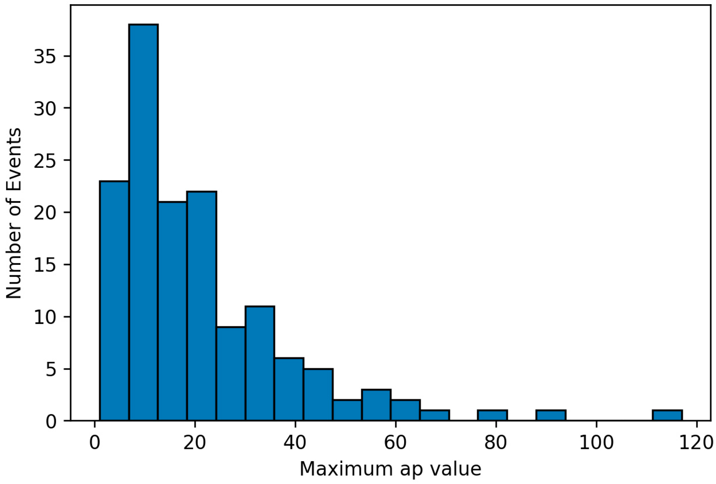
To validate the procedure described above, a database with all CMEs that affected the Earth from the year 2021 to the year 2023 was created. This database contains 146 CME events that affected the ap value from a total of 3946 CME events that occurred during this time period. From this database, 90% of the data was used as training data, while the remaining 10% was used as test data. The validation procedure was iterated 20 times, using randomly selected training and test data. The maximum ap value distribution for the selected 146 CMEs is presented in Figure 3.
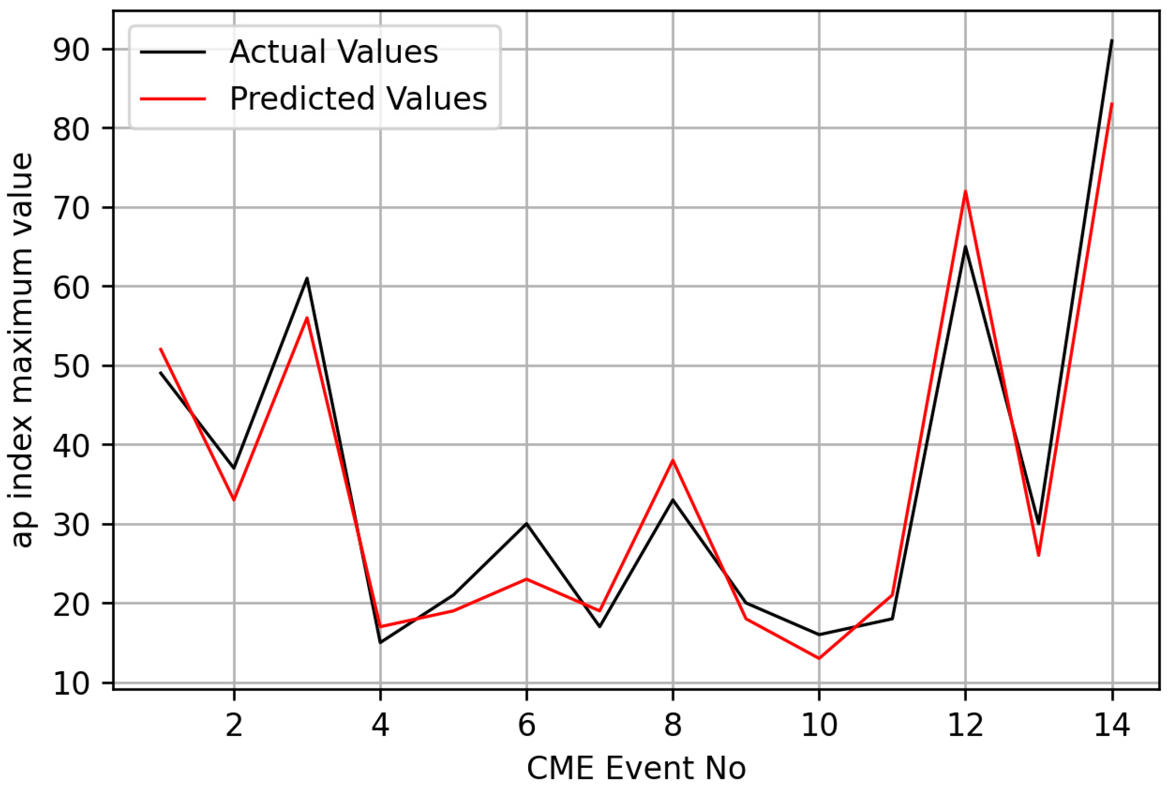
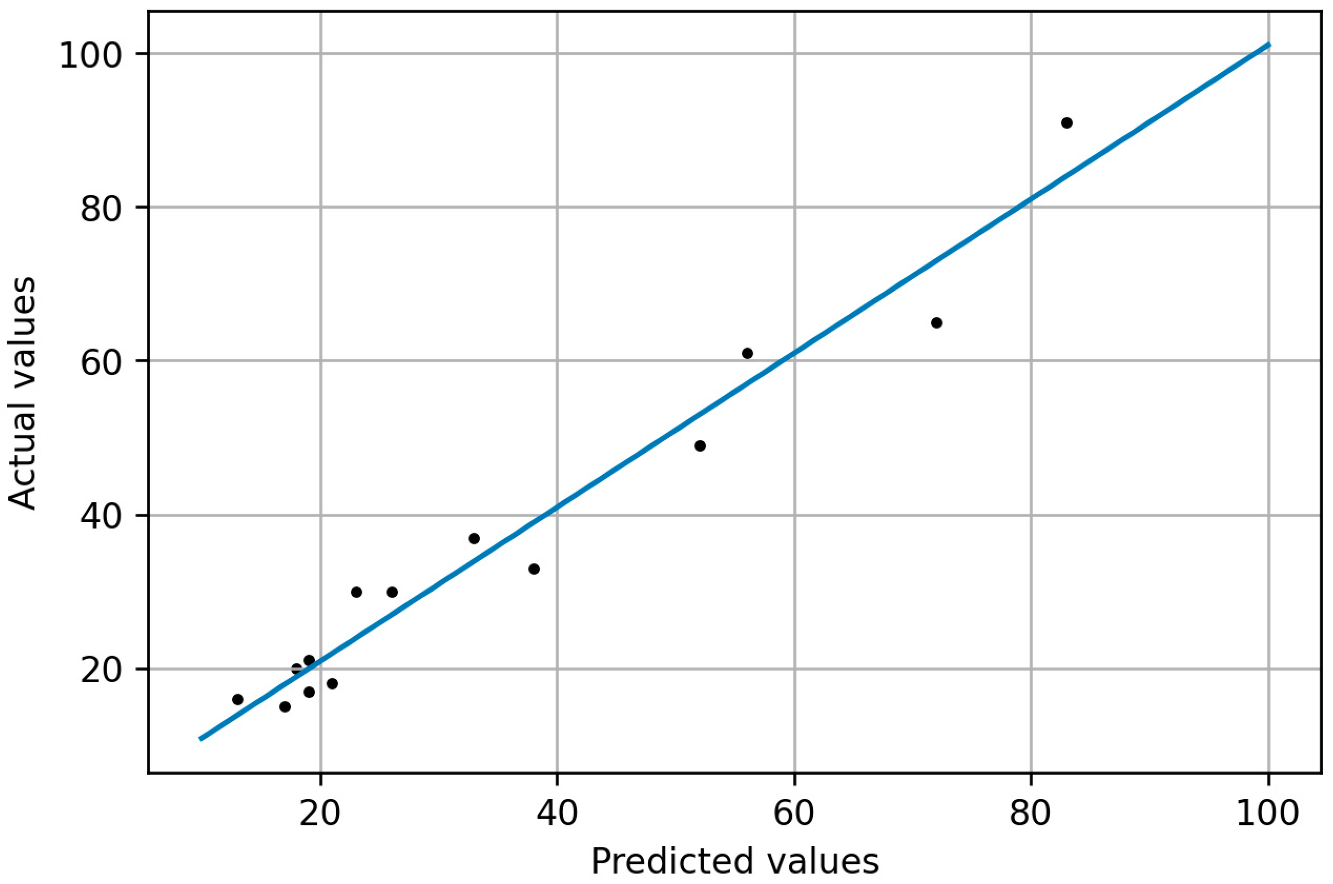
For each run of the algorithm, the actual and the predicted values of the maximum ap were compared, and the root mean square error (RMSE) values were calculated. In Figure 4 and Figure 5, the results of the first run are presented. It is clear that the algorithm can estimate ap values with high accuracy, as the results shown in Figure 5 present highly linear behavior. This linear behavior can be proven by applying best least-squares linear fit, where y = 1.0021x + 0.8525, with x being the predicted values, y the actual values and the correlation coefficient r = 0.97.
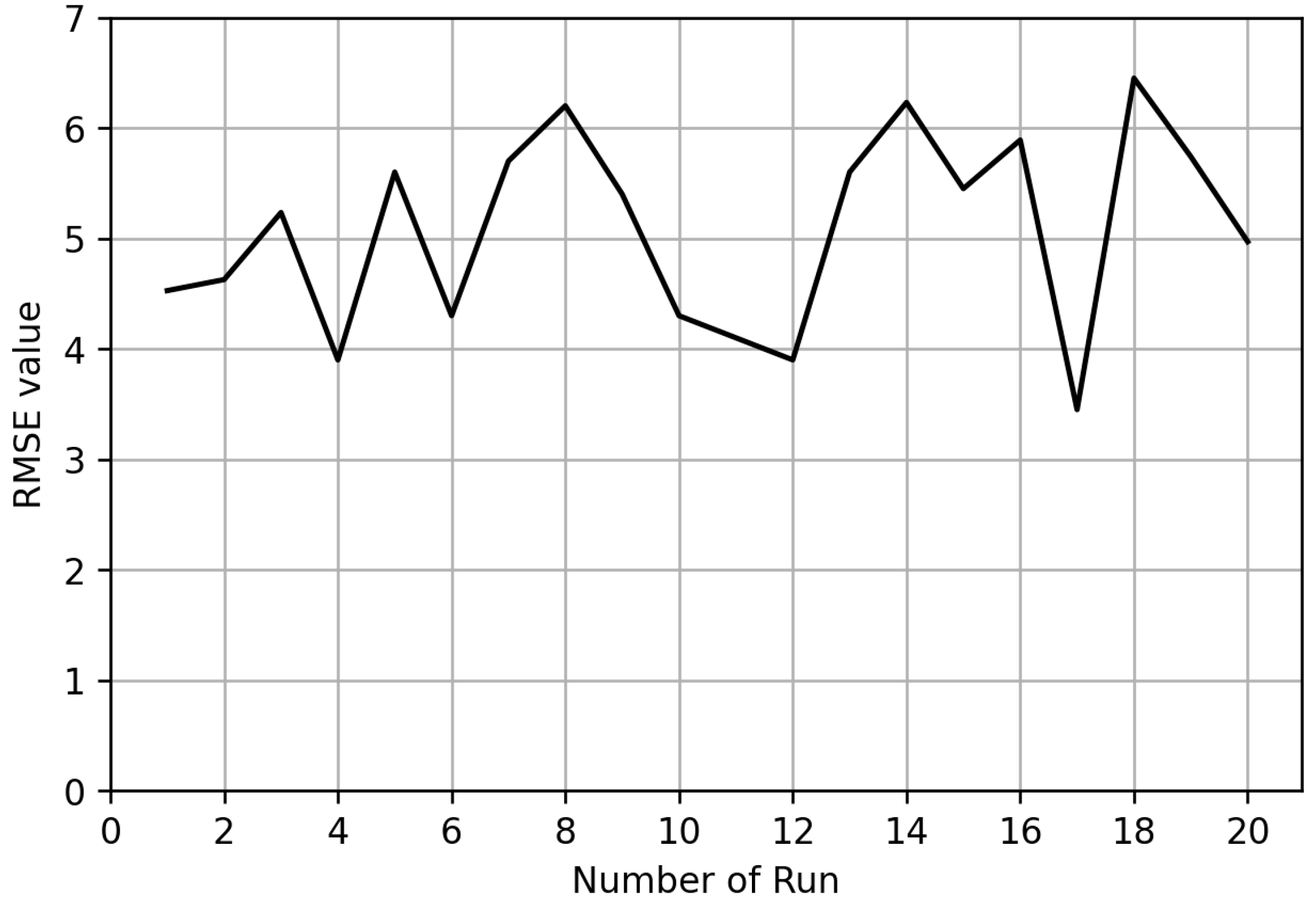
In order to complete the validation test, the above-mentioned procedure of randomly selecting training and test data was repeated multiple times. The RMSE values of every run are presented in Figure 6.
For each run, the root mean square error (RMSE) value was calculated. The results are presented in Table 1. The average value of the RMSE was estimated to be equal to 5.078. In comparison to the distribution of maximum ap values in Figure 3, the RMSE value is very low, so the accuracy of the procedure is relatively high. It is important to note that this procedure’s technique provides high accuracy and can successfully upgrade the ap Prediction tool to be fully automated.
Then, 5 new random runs, similar to the above 20 runs, were repeated in order to calculate the Pearson’s correlation coefficient r between the predicted ap index and the real ap index that were calculated for these new random runs. The results are presented in Table 2. For these five runs, the RMSE value was relatively low, and the Pearson correlation coefficient was high enough, i.e., above 0.5, to reveal that there was a strong linearity between the two variables. Furthermore, the index of agreement was also calculated, and the values extracted were high enough, i.e., over 0.9, to show high linearity between the observed and the predicted data.

5. Results from the ap Prediction Tool

5.1. The Case of the Geomagnetic Storm on 2 September 2023

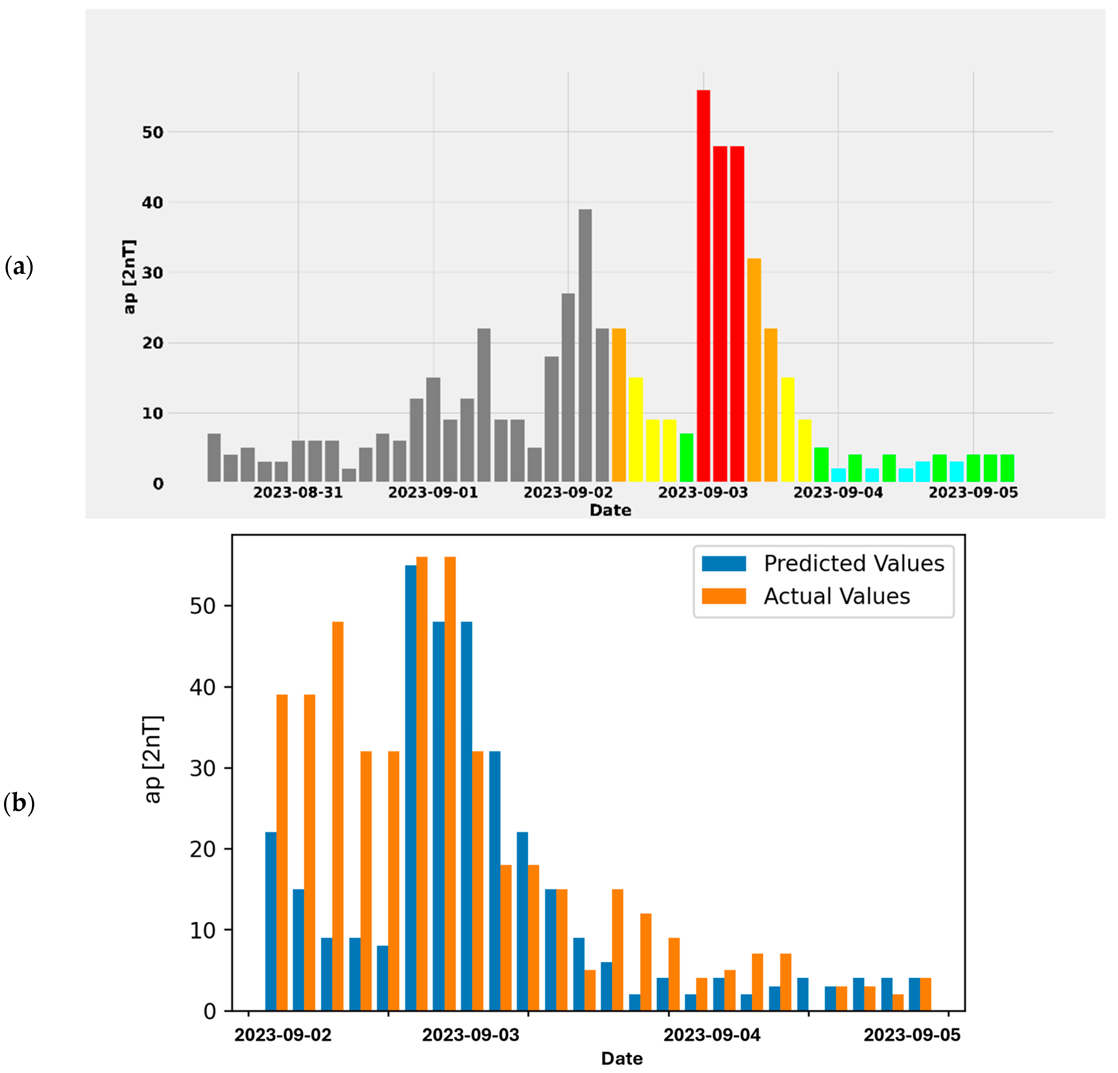
The forecaster from the Athens Cosmic ray Group (NKUA) successfully predicted the value of the apmax index during the G1-G2 geomagnetic storm which was registered on 2 September 2023 after the arrival of CMEs. A partial-halo CME was observed in LASCO C2 imagery on 30 August 2023 at 22:12 UT. This specific CME was predicted to reach Earth between 2 September 2023 at 21:46 UT and 3 September 2023 at 01:23 UT, as was shown by the EAM tool.
Following this, another fast CME was observed on 1 September 2023 at 03:24 UT, associated with a long-duration, M1.2-class solar flare. This CME was predicted to reach Earth between 2 September 2023 at 16:48 UT and 3 September 2023 at 13:30 UT according to EAM predictions.
After the first observed CME, the forecaster of the NKUA/Cosmic Ray group started to update the ap Prediction tool with data regarding the function of the CME in the file “CME_CH_data .csv’’ with the following information stated last: “2023, 09, 03, 00, 00, 56, 3’’.
The prediction output from the tool regarding the arrival of CMEs on 3 September 2023, with a maximum impact on ap at 56 nT and a potential time profile of i = 3, is presented in Figure 7a. In this figure, the cyan color indicates ap values 0–3, while the lime color indicates ap-values 4–7. The ap values from 9 to 15, 18 to 32, 39 to 154 and >179 are represented by yellow, orange, red and magenta, respectively.
In Figure 7b, it is clear that the predicted maximum ap value and the time of arrival were predicted with high accuracy. A remarkable difference is observed a few hours before the peak value of the ap. The RMSE value between the predicted and the actual values of the ap is RMSE = 13.4.

5.2. The Case of the Geomagnetic Storm on 24 September 2023

A CME was visible in SOHO LASCO C2/C3 and STEREO A COR2 on 21 September at 13:38 UT. This CME was predicted to reach Earth between 24 September at 15:22 UT and 25 September at 01:02 UT, as was shown by applying the EAM tool.
A further partial-halo CME occurred on September 22 at 02:24 UT following a filament eruption near AR 3435, triggering an M1.2 flare. This CME was predicted to reach Earth on 24 September between 20:14 UT and 23:08 UT according to EAM predictions.
The output of the tool for the geomagnetic storm on 24 September 2023 is presented in Figure 8a. Figure 8b shows that the ap Prediction tool has high accuracy regarding time arrival and the slopes before and after the time of the maximum ap value. The RMSE value for this event is RMSE = 13.57.

5.3. The Case of the Geomagnetic Storm on 5 November 2023

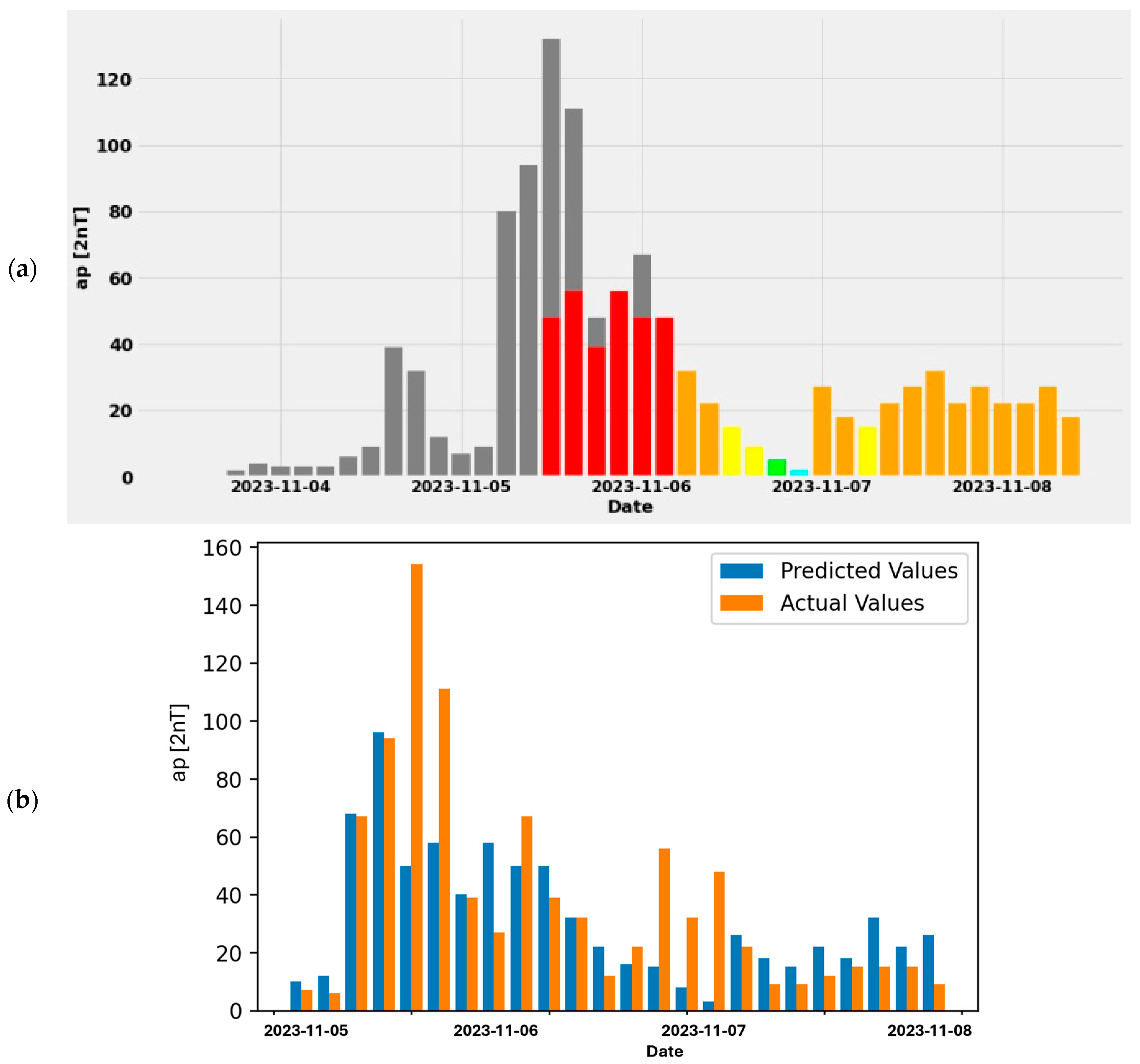
A CME was seen as a partial halo on 3 November 2023 at 05:48 UT. The eruption was likely linked to a long-duration C3.2-class solar flare that peaked on 3 November at 06:17 UT. This CME was predicted by EAM models to reach Earth on November 6 between 06:56 UT and 16:05 UT. However, the actual shock arrival was observed on 5 November at 11:45 UT (CME Scoreboard (nasa.gov), accessed on 1 July 2024).
On 5 November at 22:25 UT, solar wind speed ascended to its peak value of 530 Km/s. Furthermore, on 5 November, at 11:45 UT (http://www.swpc.noaa.gov/products/real-time-solar-wind, accessed on 1 July 2024), the southward component of Bz reached a maximum value of 37nT. The Dst index peaked with a value of −165 nT on 5 November at 20:00 UT (Real-time (Quicklook) Dst Index Monthly Plot and Table (https://www.kyoto-u.ac.jp/ja), accessed on 1 July 2024). The geomagnetic field reached strong geomagnetic storm G3 levels on 5 November 2003.
The Kp index reached a maximum value of 70 on 5 November between 15:00 and 18:00 UT, with the corresponding ap index peaking at apmax = 132. The daily Ap index value on 5 November was recorded at 62 (International Service of Geomagnetic Indices (https://www.gfz-potsdam.de/, accessed on 1 July 2024).
Following the CME that occurred on 3 November, the Cosmic Ray group/NKUA forecaster updated the file called “CME_CH_data.csv” of the ap Prediction tool by inserting the following information: “2023, 11, 05, 21, 00, 56, 3”. This information suggests that the maximum level of the ap index was anticipated on 5 November 2023 at 21:00 UT, based on the EAM model’s prediction for the CME’s arrival time. The expected ap max value was 56, and the index time, defining the time profile for the event’s duration, was specified as i = 3. The tool’s output predicting the CME’s arrival is shown in Figure 9a.
The ap index reached its max value of 154 on 5 November 2023 at 15:00–18:00 UT, as reported by GFZ (http://www-app3.gfz-potsdam.de/kp_index/qlyymm.html accessed on 1 July 2024). Consequently, the ap tool predicted the geomagnetic storm, albeit at a lower intensity and with a 3 h time discrepancy (Figure 9b). Furthermore, the algorithm had low accuracy regarding the maximum value, as the maximum value predicted was 96. This happened because of the high rarity of such high ap values in the training dataset. By inserting more similar events in the database that trains the algorithm, the results will be improved. That is the reason for the high RMSE value of this event, i.e., RMSE = 29.12.

6. Discussion and Conclusions

The accuracy of the ap Prediction tool was improved when the ap data that resulted from CME characteristics were inserted. This accuracy appears to be more pronounced in cases of G2 and G3-G4 storms, while the performance for G1 storms shows only a slight improvement. Considering that G2 and G3–G4 events occur infrequently—just once or twice per month—and that the shock arrival typically happens a few days after the event, there is sufficient time to adjust the relevant information and functions within the system. An automated tool for this process is currently under development.
(1)
A total of 3946 CMEs and their characteristics from the years 2021 to 2023 were selected for statistical analysis and the automation of the ap Prediction tool. The ap Prediction tool has to estimate which CME will arrive at the Earth and cause ap index fluctuations. This can be accomplished by importing data for all the CMEs occurring in real time from validated databases (i.e., CACTUS) and by importing data for CMEs that are expected to reach Earth (i.e., Scoreboard). Moreover, the time of arrival of the CME to the Earth is an independent process of the tool which is estimated using the EAM model of the NKUA [31,32].
(2)
As mentioned above, in the case of a CME event occurrence, the ap Prediction tool needs to be adjusted to incorporate the main characteristics of the CME to be able to extract more accurate results. This is a challenging procedure, because every CME has a different impact on ap index fluctuations, depending on its characteristics. In order to thoroughly explore this task, a dedicated algorithm was developed. Multivariate linear regression machine learning methods were employed to estimate the maximum ap value, using the angular width and median velocity of the CMEs as dependent variables.
(3)
Three selected geomagnetic storms which occurred in September and November, 2023 are presented. During these storms, which originated from CMEs, the actual values of the studied geomagnetic index presented the expected variability. The new ap Prediction tool (http://apprediction.phys.uoa.gr/ accessed on 1 July 2024) also showed a trend in space weather conditions. So, the tool can provide satisfactory results not only during the quiet periods but in the case of disturbed geomagnetic conditions, when CME events occur. In the future, this work will be extended with greater statistical analysis and improved results.
These results are possibly related to solar activity and the solar cycle phase. It is noted that the examined period is in the ascending phase and near the maximum of the current solar cycle, Solar Cycle 25. During the year 2023, the number of CMEs with and without shocks was almost constant, while in the years 2021 and 2022, this number seemed to display seasonal variation. Therefore, the automated procedure of assessing CMEs must be repeated every 2–3 years in order to provide accurate results.

Author Contributions

Software, A.S.; Data Curation, M.L.; Analysis, A.K.; Writing—Original Draft Preparation, M.L. and A.S.; Writing—Review and Editing, M.G., M.-C.P. and L.D.; Supervision, H.M. All authors have read and agreed to the published version of the manuscript.

Funding

This work received no external funding.

Institutional Review Board Statement

Not applicable.

Informed Consent Statement

Not applicable.

Data Availability Statement

Data of neutron monitors available at www.nmdb.eu (accessed on 1 July 2024).

Acknowledgments

This research was supported by the European Space Agency under the framework of the Space Weather Network: Operational and Development activities (SWESNET) under the contract number 4000134036/21/D/MRP. The authors would like to thank the cosmic ray data providers of the high-resolution Neutron Monitor Database (NMDB) and all the solar, interplanetary and geomagnetic data providers.

Conflicts of Interest

The authors declare no conflicts of interest.

References

  1. Schwenn, R. Space weather: The solar perspective. Living Rev. Solar Phys. 2006, 3, 2. [Google Scholar] [CrossRef]
  2. Lilensten, J.; Belehaki, A. Developing the scientific basis for monitoring, modelling and predicting space weather. Acta Geophys. 2009, 57, 1–14. [Google Scholar] [CrossRef]
  3. Kane, R.P. The idea of space weather. Adv. Space Res. 2006, 37, 1261. [Google Scholar] [CrossRef]
  4. Cade, W.B., III; Chan-Park, C. The Origin of Space Weather. Space Weather 2005, 13, 99–103. [Google Scholar] [CrossRef]
  5. Parks, G.K. Physics of Space Plasmas; Addison-Wesley Publishing Company: Boston, MA, USA, 1991. [Google Scholar]
  6. Daglis, I.A. Space Storms and Space Weather Hazards; NATO ASI Series; Springer: Berlin/Heidelberg, Germany, 2001. [Google Scholar]
  7. Hanslmeier, A. The Sun and Space Weather; Astrophysics and Space Science Library; Springer: Berlin/Heidelberg, Germany, 2007; Volume 347. [Google Scholar]
  8. Ramesh, K.B. Solar cycle variation of the occurrence of geomagnetic storms, Solar drivers of interplanetary and terrestrial disturbances. ASP Conf. Ser. 1996, 95, 462–469. [Google Scholar]
  9. Zhang, J.; Richardson, I.G.; Webb, D.F.; Gopalswamy, N.; Huttunen, E.; Kasper, J.C.; Nitta, N.V.; Poomvises, W.; Thompson, B.J.; Wu, C.C.; et al. Correction to Solar and interplanetary sources of major geomagnetic storms (Dst <= -100 nT) during 1996–2005. J. Geophys. Res. 2007, 112, A12103. [Google Scholar] [CrossRef]
  10. Kallenrode, M.B. Space Physcs: An Introduction to Plasmas and Particles in the Heliosphere and Magnetospheres; Springer: Berlin/Heidelberg, Germany, 1998. [Google Scholar]
  11. Collado-Villaverde, A.; Muñoz, P.; Cid, C. Classifying and bounding geomagnetic storms based on the SYM-H and ASY-H indices. Nat. Hazards 2024, 120, 1141–1162. [Google Scholar] [CrossRef]
  12. McPherron, R. Predicting the Ap index from past behavior and solar wind velocity. Phys. Chem. Earth 1999, 24, 45–56. [Google Scholar] [CrossRef]
  13. Bartels, J.; Heck, N.H.; Johnston, H.F. The three-hour range index measuring geomagnetic activity. J. Geophys. Res. 1939, 44, 411–454. [Google Scholar] [CrossRef]
  14. Rostoker, G. Geomagnetic Indices. Rev. Geophys. Space Phys. 1972, 10, 935–950. [Google Scholar] [CrossRef]
  15. Thomsen, M.F. Why Kp is such a good measure of magnetospheric convection. Space Weather 2004, 2, S11004. [Google Scholar] [CrossRef]
  16. Menvielle, M.; Iyemori, T.; Marchaudon, A.; Nose, M. Geomagnetic indices. In Geomagnetic Observations and Models; Mandea, M., Korte, M., Eds.; IAGA Special Sopron Book Series 5; Springer: Dordrecht, The Netherlands, 2011; pp. 183–228. [Google Scholar] [CrossRef]
  17. Stassinakis, A.; Livada, M.; Gerontidou, M.; Tezari, A.; Mavromichalaki, H.; Paouris, E.; Makrantoni, P. Forecast of the Geomagnetic Index ap during CME Events; European Space Weather Week: Coimbra, Portugal, 2023. [Google Scholar]
  18. Wang, J.; Luo, B.; Liu, S.; Shi, L. A machine learning-based model for the next 3-day geomagnetic index (Kp) forecast. Front. Astron. Space Sci. 2023, 10, 1082737. [Google Scholar] [CrossRef]
  19. Horne, R.B.; Phillips, M.W.; Glauert, S.A.; Meredith, N.P.; Hands, A.D.P.; Ryden, K.A.; Li, W. Realistic Worst Case for a Severe Space Weather Event Driven by a Fast Solar Wind Stream. Space Weather 2018, 16, 1202–1215. [Google Scholar] [CrossRef] [PubMed]
  20. Mourenas, D.; Artemyev, A.V.; Zhang, X.J. Impact of Significant Time-Integrated Geomagnetic Activity on 2-MeV Electron Flux. J. Geophys. Res. Space Phys. 2019, 124, 4445–4461. [Google Scholar] [CrossRef]
  21. Hua, M.; Bortnik, J.; Chu, X.; Aryan, H.; Ma, Q. Unraveling the Critical Geomagnetic Conditions Controlling the Upper Limit of Electron Fluxes in the Earth’s Outer Radiation Belt. Geophys. Res. Lett. 2022, 49, e2022GL101096. [Google Scholar] [CrossRef]
  22. Lockwood, M.; Chambodut, A.; Finch, I.D.; Barnard, L.A.; Owens, M.J.; Haines, C. Time-of-day/time-of-year response functions of planetary geomagnetic indices. Space Weather Space Clim. 2019, 9, A20. [Google Scholar] [CrossRef]
  23. Hochreiter, S.; Schmidhuber, J. Long Short-Term Memory. Neural Comput. 1997, 9, 1735–1780. [Google Scholar] [CrossRef]
  24. Yu, Y.; Si, X.; Hu, C.; Zhang, J. A review of recurrent neural networks: LSTM cells and network architectures. Neural Comput. 2019, 31, 1235–1270. [Google Scholar] [CrossRef]
  25. Bailey, R.L.; Leonhardt, R.; Moestl, C.; Beggan, C.; Reiss, M.A.; Bhaskar, A.; Weiss, A.J. Forecasting GICs and Geoelectric Fields from Solar Wind Data Using LSTMs: Application in Austria. Space Weather 2022, 20, e2021SW002907. [Google Scholar] [CrossRef]
  26. Camporeale, E. The Challenge of Machine Learning in Space Weather: Nowcasting and Forecasting. Space Weather 2019, 17, 1166–1207. [Google Scholar] [CrossRef]
  27. Devos, A.; Verbeeck, C.; Robbrecht, E. Verification of space weather forecas0ng at the regional warning center in Belgium. Space Weather. Space Clim. 2014, 4, A29. [Google Scholar] [CrossRef]
  28. Jolliffe, I.T.; Stephenson, D.B. Forecast Verification. A Practioners Guide in Atmospheric Science, 2nd ed; Wiley-Blackwell: Hoboken, NJ, USA, 2012. [Google Scholar]
  29. Hu, A.; Camporeale, E.; Swiger, B. Multi-hour-ahead Dst index prediction using multifidelity boosted neural networks. Space Weather 2023, 21, e2022SW003286. [Google Scholar] [CrossRef]
  30. Liemohn, M.W.; McCollough, J.P.; Jordanova, V.K.; Ngwira, C.M.; Morley, S.K.; Cid, C.; Tobiska, W.K.; Wintoft, P.; Ganushkina, N.Y.; Welling, D.T.; et al. Model evaluation guidelines for geomagnetic index predictions. Space Weather 2018, 16, 2079–2102. [Google Scholar] [CrossRef]
  31. Paouris, E.; Mavromichalaki, H. Effective Acceleration Model for the arrival time of interplanetary shocks driven by coronal mass ejections. Sol. Phys. 2017, 292, 180. [Google Scholar] [CrossRef]
  32. Paouris, E.; Mavromichalaki, H. Interplanetary coronal mass ejections resulting from Earth-Directed CMEs Using SOHO and ACE Combined Data during Solar Cycle 23. Sol. Phys 2017, 292, 30. [Google Scholar] [CrossRef]
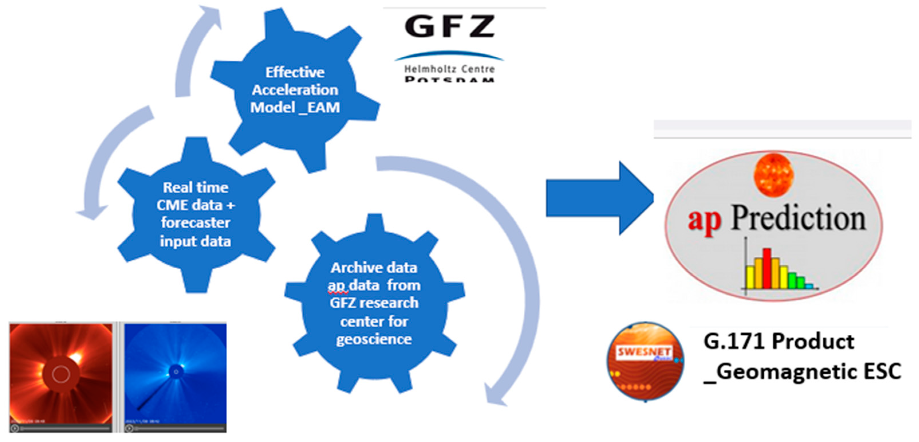
Figure 1. Block diagram of the ap Prediction tool (https://swe.ssa.esa.int/ap_Prediction-federated accessed on 1 July 2024).
Atmosphere 15 01073 g001
Figure 2. Fields of CCMC with CME events that are expected to affect the Earth.
Atmosphere 15 01073 g002
Figure 3. Distribution of the 146 CME events that were used in this work.
Atmosphere 15 01073 g003
Figure 4. Actual and predicted values of the ap maximum during the first run of the algorithm (14 events).
Atmosphere 15 01073 g004
Figure 5. Actual values vs. predicted values of the ap index of the first run of the algorithm.
Atmosphere 15 01073 g005
Figure 6. The RMSE values of all the runs of the algorithm (20 runs).
Atmosphere 15 01073 g006
Figure 7. Predicted values extracted directly from the ap tool (a) the cyan color indicates ap values 0–3, while the lime color indicates ap-values 4–7. The ap values from 9 to 15, 18 to 32, 39 to 154 and >179 are represented by yellow, orange, red and magenta, respectively; predicted and real ap values for the next 72 h from 2 September 2023 (b).
Atmosphere 15 01073 g007
Figure 8. Predicted values extracted directly from the ap tool (a) the cyan color indicates ap values 0–3, while the lime color indicates ap-values 4–7. The ap values from 9 to 15, 18 to 32, 39 to 154 and >179 are represented by yellow, orange, red and magenta, respectively; predicted and real ap values for the next 48 h from 24 September 2023 (b).
Atmosphere 15 01073 g008
Figure 9. Predicted values extracted directly from the ap tool (a); predicted and real ap values for the next 72 h from 5 November 2023 (b).
Atmosphere 15 01073 g009
Table 1. The RSME values of each run of the algorithm.
RUN1RUN2RUN3RUN4RUN5RUN6RUN7RUN8RUN9RUN10
4.5274.6275.2343.9205.6124.3275.6986.2345.4314.312
RUN11RUN12RUN13RUN14RUN15RUN16RUN17RUN18RUN19RUN20
4.1803.9435.6186.2375.54515.8933.4576.4485.7414.973
Table 2. RMSE values and correlation coefficient r.
RUN1RUN2RUN3RUN4RUN5
RMSE5.2374.9836.1127.3285.913
r0.780.790.830.590.71
Index of agreement0.920.970.990.90.92
Disclaimer/Publisher’s Note: The statements, opinions and data contained in all publications are solely those of the individual author(s) and contributor(s) and not of MDPI and/or the editor(s). MDPI and/or the editor(s) disclaim responsibility for any injury to people or property resulting from any ideas, methods, instructions or products referred to in the content.