1. Introduction
Flashiness is the frequency and rapidity in which streamflow changes [
1] as defined in equation 1. Flashier responses after storm events cause a more concentrated flood wave, accompanied by higher flows [
2], which can be attributed to more impervious land (e.g., urbanization) or more intense rainfall. This can have serious implications in flood risk, with the potential to cause widespread damage and fatalities [
3]. Climate change is projected to influence the magnitude and timing of hydrological extremes, with increases in the future expected [
4,
5]. In the UK, annual damages from flooding are expected to increase by 27% by 2050, under a 2 °C by 2100 warming scenario (and 44% for 4 °C warming) [
6]. Therefore, the analysis of flashiness across Great Britain can offer additional insights into the rapidity and frequency of flood events.
Flashiness has also been used to estimate diffuse source pollution concentrations in rivers, with important ecological ramifications. In their analysis of pesticide discharge in the US, Gustafson et al. (2004) [
7] relate the concentration of pesticides in rivers to the sharpness of its hydrograph, i.e., the rate of increase in flow on a day-to-day basis. Similarly, Ulen et al. (2016) [
8] found flashiness to best explain the phosphorous losses in a Swedish farm. Changes to the flashiness can thus provide early indications of pollution loads in rivers which can make it a useful metric for tracking river pollution at a national scale. In UK river systems, despite efforts to improve river quality, poor ecological status is still persistent [
6], with rivers around urban areas having the worst quality, and continued issues surrounding intensive agricultural practices. Overall, flashiness characterises a key component in hydrological regimes [
1], focusing on flow variability rather than simply flow magnitude. Given that freshwater ecosystems are particularly vulnerable to flow regime changes [
9], changes in flashiness could be detrimental to river health.
River flashiness has been described using several metrics, such as Peaks Over Thresholds (POT) [
3], time-to-rise TR, characteristic flood duration θ [
2] or even ratio measures like 20R80 [
10]—the ratio of flows exceeded 80% of the time to those exceeded 20% of the time. Nevertheless, this study will restrict itself to the widely used Richards–Baker flashiness index (
) [
1], for its simplicity and potential to detect temporal trends relative to other metrics. It is calculated as follows [
1]:
where q
i is the mean daily flow, and n
y is the number of days in that year. Essentially, it corresponds to the sum of day-to-day variations in streamflow, normalised by the total yearly streamflow.
has been used to explore the water balance within catchments, specifically the interplay between precipitation and storage, with relevance to water resource management. For instance, elements such as rainfall intensity, snow cover and geology were used by Holko et al. (2011) [
11] to describe the spatial changes in flashiness in Austrian and Slovakian mountain streams. Importantly, this intricate dynamic between storage and precipitation also varies with time [
1,
11]). In large scale studies, these temporal changes in flashiness have been detected using the Mann–Kendall test for monotonic trends [
11], yet sudden changes or “breakpoints” in flashiness may also exist. For example, through visual analysis, Baker et al. (2004) [
1] observed a distinct drop in flashiness after the construction of the dam in East Fork, Whitewater River, USA. In the same vein, a significant increase in winter flashiness was observed after the construction of hydropower stations in St. Micheal-Mur, Austria [
11]. Using a Mann–Kendall trend test on such cases would overlook their significant breakpoints.
The majority of studies exploring
have centred on the USA [
1,
12], with some in mainland Europe [
11,
13]. There has been limited exploration of
in catchments in the UK until now. It is not clear why this may be, although there is a strong focus on understanding the Base Flow Index (BFI) of rivers in Great Britain. BFI is a derived flow metric which is used to understand the proportion of the river runoff that originates from stored sources, including example soils, and is related to flashiness but focusses on the low flow component of a river response rather than the high flow component. However, given the implications of
in flooding, river health and water resource management, a national study across Great Britain could highlight vulnerable river basins, and inform future adaptation planning.
As such, this study aims to offer a detailed spatio-temporal analysis of flashiness in Great Britain, answering the following questions:
- (a)
What are the spatial patterns of flashiness in Great Britain? Such patterns can help regional flood alleviation plans.
- (b)
Can potential predictors for flashiness be identified? Predictors can expand findings to ungauged river basins.
- (c)
Are there common breakpoints or trends in flashiness on annual or seasonal scales? Understanding common trends can identify vulnerable regions, and focus future studies on potential drivers of change.
This will be the first analysis of river flashiness across mainland Great Britain, and as such provides novel insights into the behaviour of river catchments both within a year, as well as over a 50 year period across the country.
2. Methods
In order to assess spatio-temporal patterns in flashiness in Great Britain, the methods used in this study can be split into two sets. The first set of methods targets spatial patterns in flashiness and potential predictors, using cluster analysis and random forest analysis, respectively (
Section 2.1 and
Section 2.2). For this first set, a 30-year study period was used, which is often used as a standard period of time in hydrology to explore trends in fluctuating timeseries. By contrast, the second set of methods addresses temporal analysis, using the Pettitt test for breakpoints and the Mann–Kendall trend test (appropriate for non-normally distributed data), as well as cluster analysis to assess the timing of flashy events (
Section 2.3)—here, a 50-year study period was used. Using a longer timeseries is beneficial for this analysis in order to detect trends and break points; however, a balance needed to be struck between the number of gauges available with long complete river flow series and the length of period of analysis; hence, 50 years was the optimal length. For both sets of methods, the magnitude of flashy events as well as the timing of flashy events are considered. An overview of the methods employed can be seen in
Figure 1.
2.1. Spatial Patterns in Flashiness
Flow data: Flow data and metadata were sourced from the rnrfa package in R [
14], providing gauged daily flow (GDF), monthly rainfall as well as a multitude of catchment descriptors from the UK National River Flow Archive. All data and information for these gauges are freely available through the rnrfa package in R. The 513 gauge stations used for spatial analysis were selected based on whether they contained complete GDF data for the 30 years spanning 1 October 1990 to 30 September 2020. Thirty-year standard reference periods, outlined by the World Meteorological Organisation, have been used in hydro-meteorological contexts to smooth out anomalous years, as well as include longer cyclical weather events [
15], such as the North Atlantic Oscillation. To reduce lag-one autocorrelation, water years were used instead of calendar years, spanning from the 1st of October to the 30th of September (the following year).
Magnitude and Shape: In order to separate flashiness magnitude from the timing of flashy events, catchments can be described both by flashiness magnitude and by “shape” [
16]. To capture flashiness magnitude, the Richards–Baker flashiness index was used, calculated on a yearly basis. Over the thirty-year period, the magnitude is summarized by the average yearly flashiness
and standard deviation σ
RBI.
To capture the “shape” of flashiness over an average water year, the average monthly flashiness (
m) was computed for the 30-year period. As such, each month of the water year had its own mean flashiness, for each station. Next the average monthly flashiness was standardized over the twelve months for each station individually, thereby removing magnitude from the regime and isolating only the “shape”. The monthly flashiness was computed as follows:
where q
i is the mean daily flow, n
m is the number of days in the month and n
y is the number of days in that year. Effectively, this corresponds to the average day-to-day variation in river flow in a particular month, normalized by the average daily flow for that water year. Normalizing by the yearly average flow is performed to quantify the monthly flashiness in the context of that particular water year and allows comparison to other studies [
1,
3,
8]. By contrast, if it were normalized by the mean monthly flow, small peaks in flow could still create a large flashiness index if the mean monthly flow is low as well, potentially causing misleading regime shapes.
Clustering: Taking the resultant flashiness “shapes” of all stations, a two-stage clustering procedure was conducted. In this instance, clustering can condense all shapes into a set of classes, used to outline spatial patterns in the timing of flashy events. For the two-stage clustering, hierarchical clustering is first performed (Stage 1) followed by k-means clustering to reorganise clusters around their centroids (Stage 2). The cluster package in R was used for both stages [
17].
In Stage 1, four linkage methods were considered: Average Linkage, Single Linkage, Complete Linkage and Ward’s method. The linkage method with the highest agglomerative coefficient was selected, indicating the most compact clusters. Next, to determine the number of clusters to select in Stage 1, the Average Silhouette method and the Elbow method were used.
With the number of clusters selected, k-means clustering (Stage 2) was then performed using the cluster centroids as the starting position of the algorithm. For interpretation of the results, the average rainfall shapes were also computed, using the same procedure. Catchment rainfall was extracted from the catchment mean monthly rainfall (CMR) series in rnrfa. The rainfall series spans only to December 2017, so the 1990–2016 water years were used for the averaged rainfall shapes.
2.2. Random Forest Analysis
Random forests are an ensemble of decision trees with the key characteristic that at each node split, a random subset of features (or predictor variables) is considered, thereby promoting variety in the trees [
18]. Each tree in the ensemble is created using bootstrap aggregating, or bagging—i.e., selecting a random subset of data points (with replacement) to train each tree. The data points that are not selected can then be used to test the accuracy of the ensemble, and offer a metric for fine-tuning the random forest: the Out-of-Bag (OOB) Error [
19]. Given a random forest, the importance of each feature can be computed, which corresponds to the average gain in accuracy of the model at each node involving said feature [
18]. Following the method described by Gannon et al. [
12], this study uses random forests to compute the importance of certain catchment characteristics in predicting flashiness [each average shape class (from
Section 2.1)].
Predictor Variables: The predictor variables to train the random forest were selected from the available catchment descriptors in the rnrfa package in R [
14]. This included metrics for altitude 6 and slope (mean altitude, 10-percentile-altitude…), metrics for catchment size and location (catchment-area, latitude…), subsurface permeability (low-perm-superficial, high-perm-bedrock…), rainfall (rmed-1h, rmed-1d…) and land cover (urbloc-2000, lcm2007-arablehorticultural, FARL…). The catchment mean rainfall over the study period was computed separately using the catchment mean monthly rainfall (CMR) series in rnrfa between the 1990 and 2016 water years, for each station. Of the full 513 stations with an
calculated, one station was omitted from the random forest analysis (ID: 18011), as it had no FEH catchment descriptors available. Missing values in the UKCEH Land Cover Maps were set to 0; based on inspection, these were percentages of land cover too small to be computed. The urban location index (urbloc-2000) was removed as a potential predictor, since it can only be computed for catchments with urban/suburban areas [
20]. Next, a correlation matrix was computed for the catchment features using Spearman’s correlation coefficient (ρ), and variables were selectively removed until no two variables had a correlation coefficient over 0.7. This resulted in a final set of 18 potential predictors.
Training and Tuning The random forests were grown using the ranger package in R [
21]. First, the number of trees was determined, running past the point where the OOB error converges (giving 500 trees). Next, a grid search was conducted to determine the following hyperparameters: the number of variables to select at each node (10), the sample size of data to train on (78%) and the minimum node size to split at (6). With the hyperparameters determined, the random forests were created for each region, and the feature importance was extracted. The same set of hyperparameters was used for each region.
2.3. Temporal Analysis
Flow data: For the timeseries analysis, 208 stations were selected such that they had complete Gauged Daily Flow (GDF) datasets in the 50-year period beginning on 1 October 1970 and ending on 30 September 2020. GDF data were once again sourced from the rnrfa package in R [
14]. A 50-year period was chosen (rather than the shorter 30-year period in
Section 2.1/
Section 2.2) to examine long-term trends. 50-year analysis achieved the right balance between the number of stations where data were available (to ensure coverage of Great Britain), and the duration of the timeseries [
22].
Breakpoint and trend tests: Using this 50-year period, the yearly
timeseries (in water years) was computed for each station, using Equation (1). The Pettitt test was used to capture significant breakpoints in flashiness, with
p < 0.05. To find significant trends, the Mann–Kendall trend test was used over the study period, with
p < 0.05. Both the Mann–Kendall trend test and Pettitt test are non-parametric, making them well suited in hydro-meteorological timeseries [
23,
24]. For breakpoints, the magnitude of the step-change in median before and after the breakpoint was expressed as follows:
where m is the median
over the full timeseries, m
1 is the median
before the breakpoint (including the breakpoint year), and m
2 is the median
after the breakpoint. The average lag-one autocorrelation in the flashiness timeseries was 0.21; therefore, it is expected that the Type I error in breakpoints is not significant, and pretreatment was not employed.
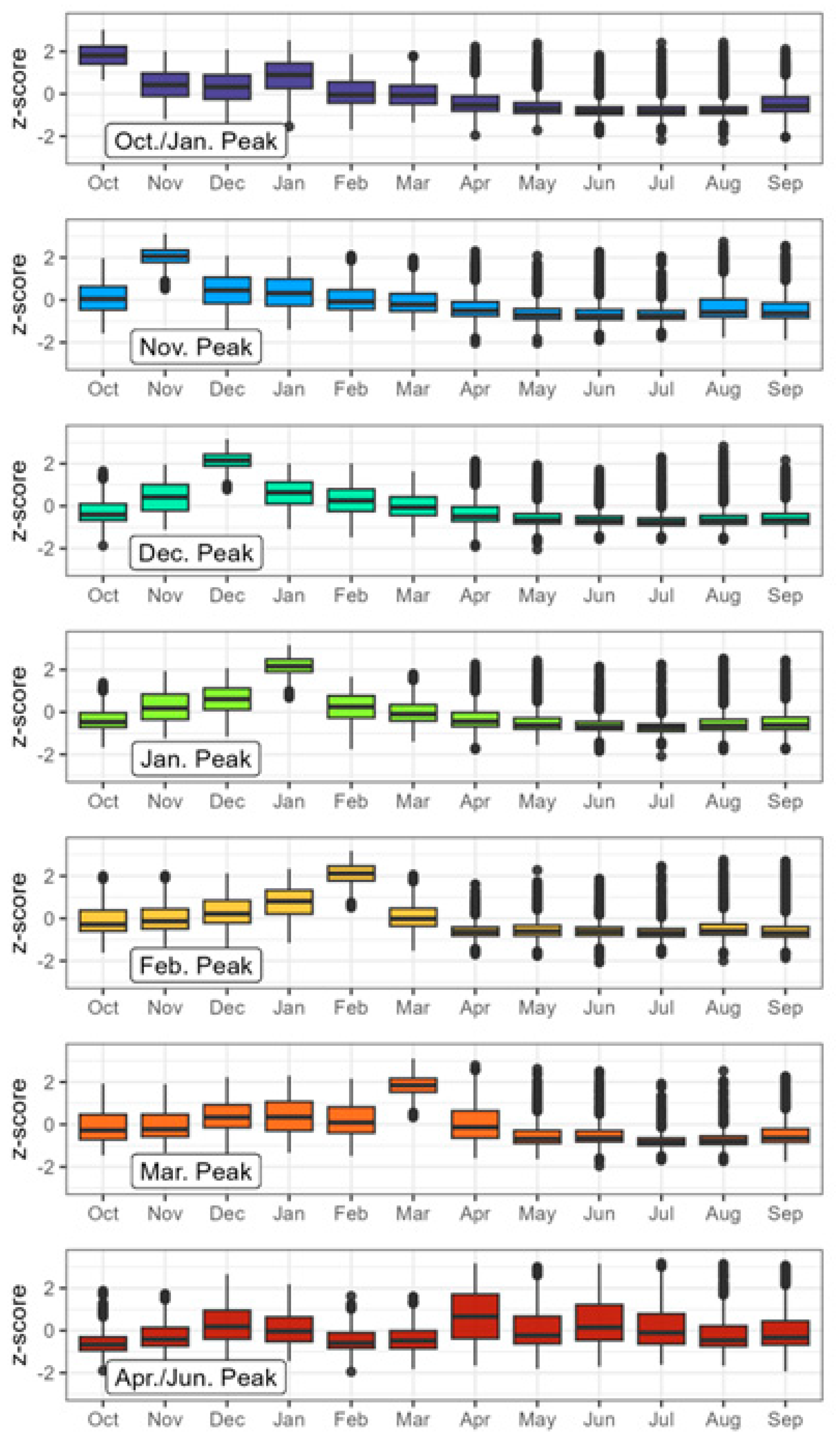
Shape stability: Whilst the timeseries analysis provides an overview of how the flashiness magnitude has varied over time, it does not consider how the flashiness regime shape has varied in time, i.e., the timing of flashy events during a water year. To provide this additional layer to the temporal analysis, the two-stage classification was once again administered [
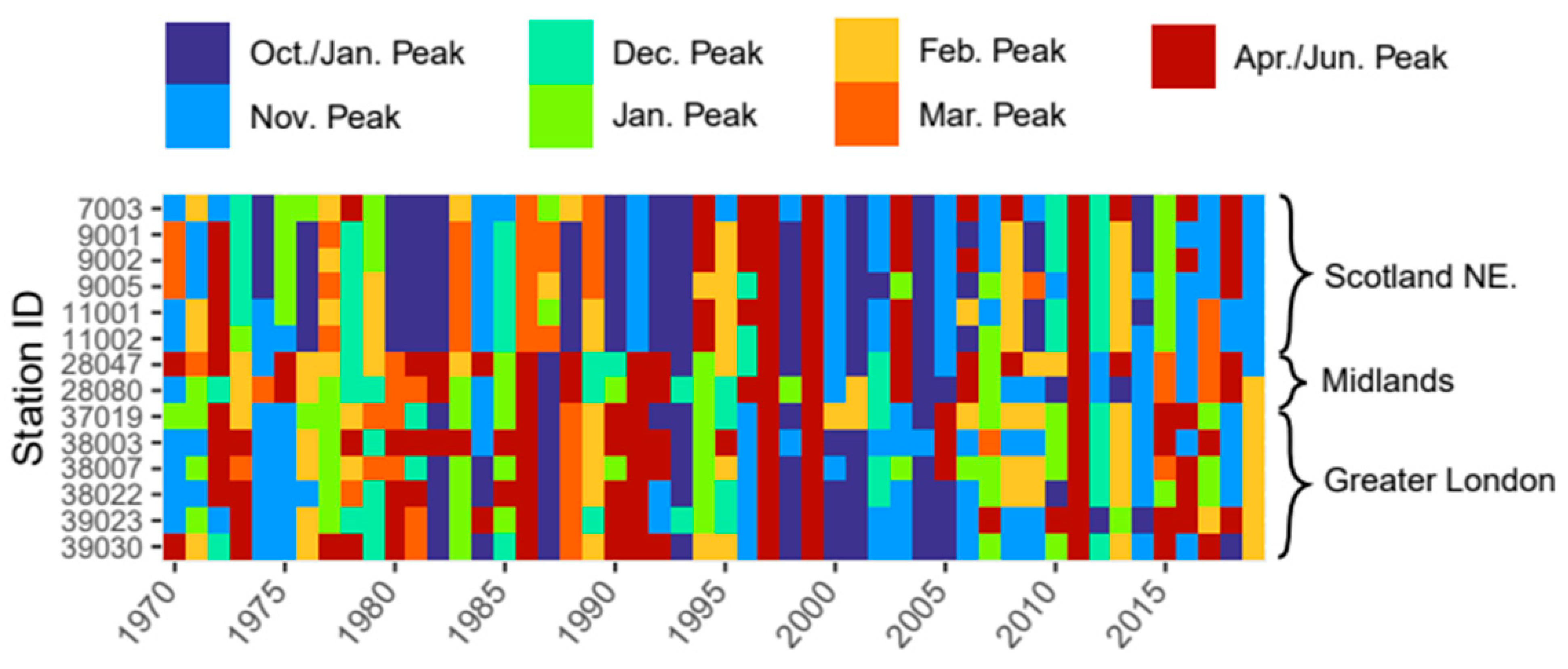
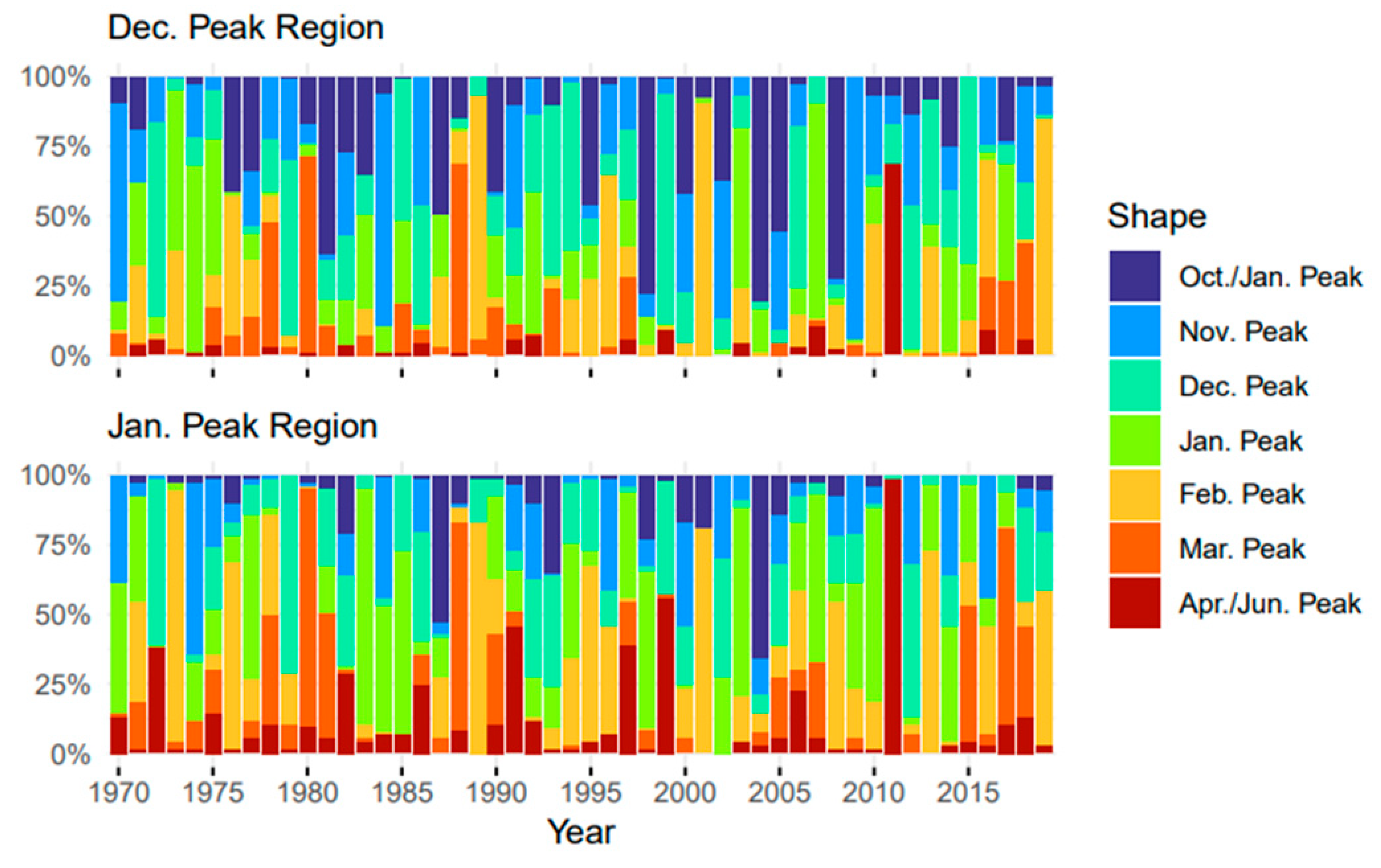
16]. This time, a standardized flashiness shape was computed for each year individually, for each station, creating a total of 10,400 shapes (i.e., 208 stations × 50 years). The resulting 10,400 shapes were then clustered using the two-stage cluster analysis, to obtain a set of common yearly flashiness shapes. From this point, by reassigning each initial yearly shape to its new shape class, a timeseries of shapes for each station was calculated. For the two-stage clustering, the fastcluster package in R was used [
25].
4. Discussion
The aim of this study is determining how flashiness varies spatially and temporally in Great Britain.
4.1. Spatial Analysis of Flashiness across Great Britain
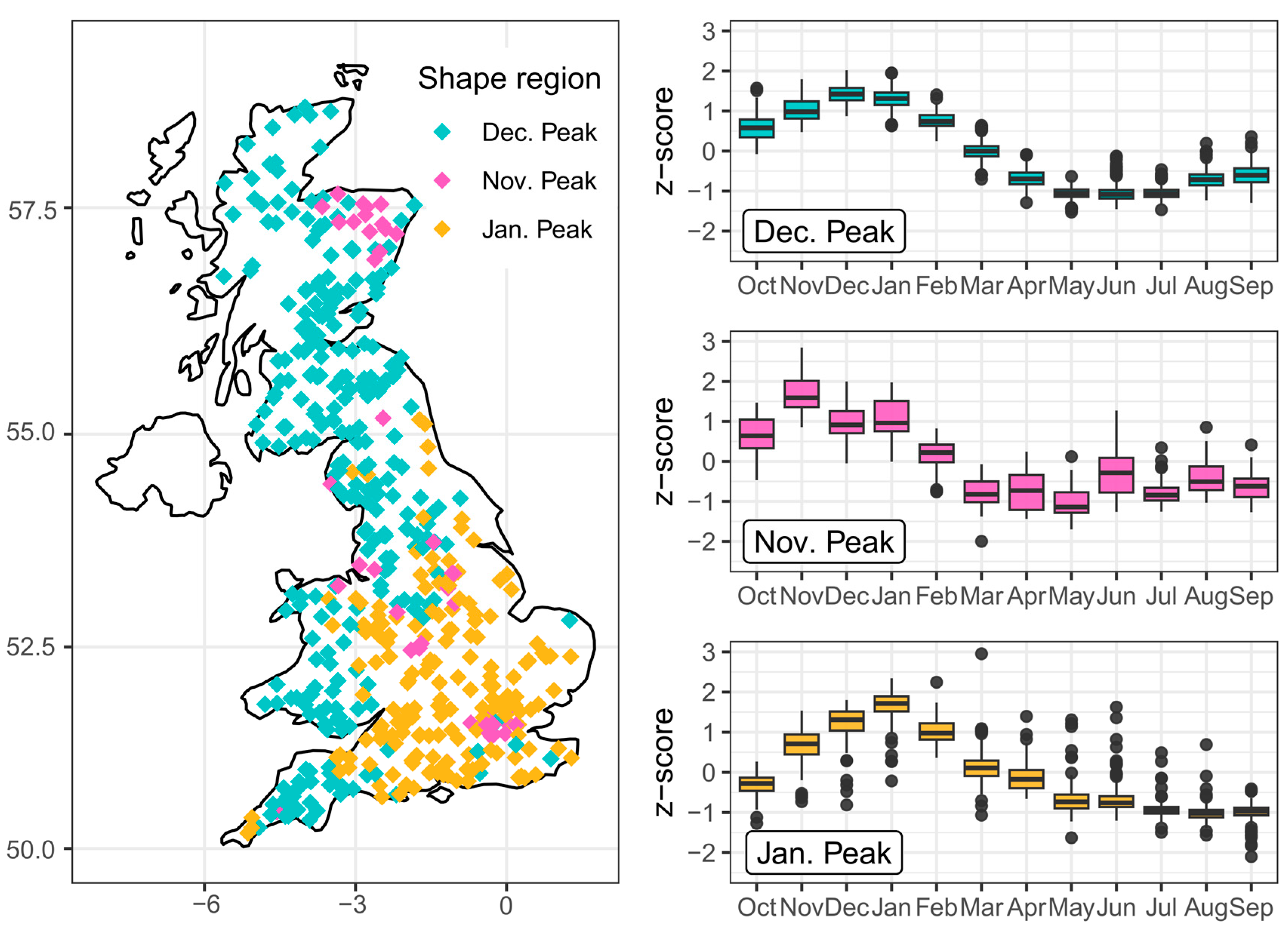
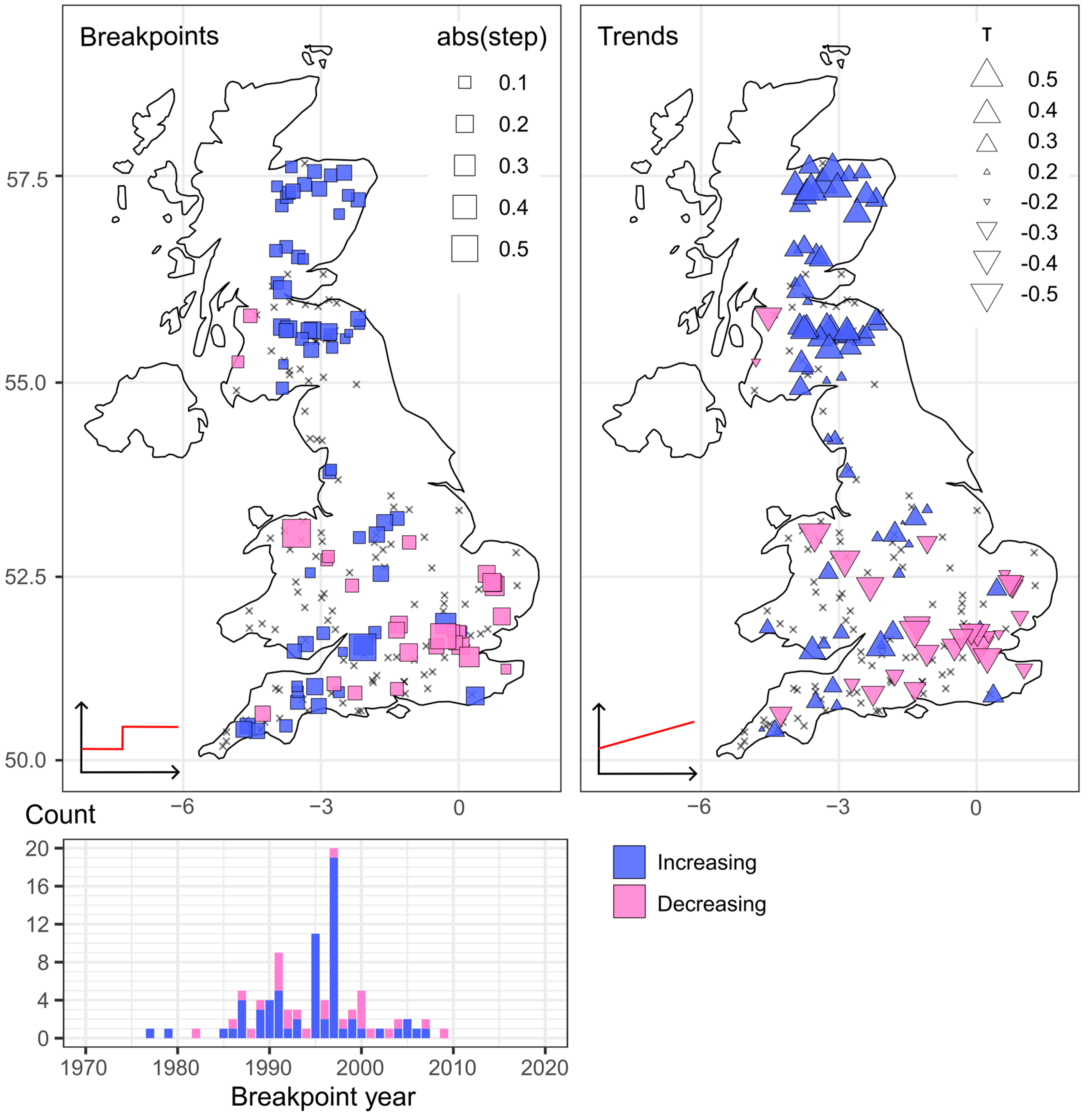
Spatially, it was found that, averaged over the most recent 30-year period, flashiness follows a general west-coast–east-coast gradient, being higher in the west, although spatial anomalies are present. Based on a random forest analysis, key predictors for flashiness were found to be region dependent, with an overall strong link to soil composition. This demonstrates the importance of water storage in relation to flashiness in Great Britain. Temporally, significant breakpoints and/or trends in flashiness were detected in over 50% of the 208 catchments considered over a 50-year period. The north-east and south-west of Great Britain largely showed increases in flashiness, whilst Greater London was characterised by decreases in flashiness. These significant temporal changes have implications in river health as well as flooding. On a seasonal scale, flashiness was generally shown to oscillate between autumn/winter peaks and spring peaks, with no clear trends visible.
4.1.1. Primary Predictors for Flashiness
Gannon et al. [
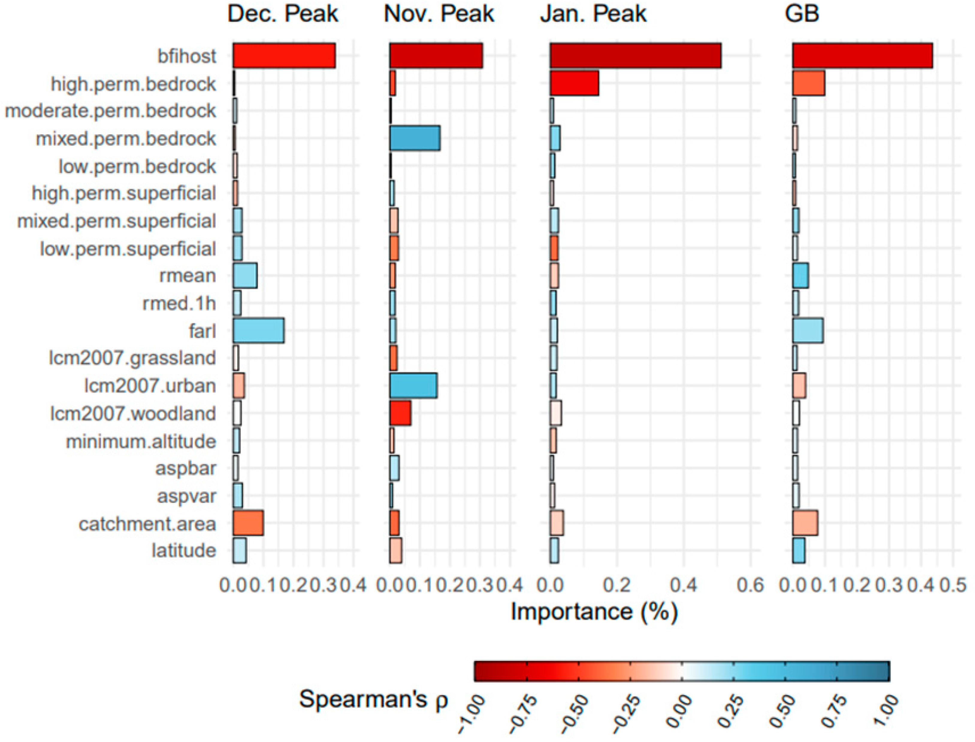
12] demonstrated that key predictors in flashiness vary by region when observing the continental US; this study has demonstrated that Great Britain is similar. Although grouping all stations in GB together increased the overall random forest model accuracy, it also smoothed out the importance of key regional predictors in flashiness.
Notably, in the south-east, mean flashiness can be predicted almost entirely by BFIHOST (the base flow index per HOST soil class). Meanwhile, the north and west of GB require additional parameters, namely FARL (flood attenuation for reservoirs and lakes) and catchment area, to accurately predict mean flashiness. The “Nov. Peak” region, despite having a lower model accuracy R
2 = 0.64, showed a reliance on urban area and mixed permeability bedrock, as well as BFIHOST. For comparison, Gannon et al. [
12] demonstrated that climatic features (e.g., potential evapotranspiration, annual precipitation) were the primary predictors for flashiness in the continental United States. However, in many regions, human impacts, land cover, subsurface and watershed structure still composed over 50% of the model importance. In Great Britain, this study suggests that climate presents less importance in predicting flashiness, with a stronger influence from soil conditions. However, the set of catchment features available to train the random forest model play a large influence in the final key predictors. Gannon et al. [
12] had only one catchment descriptor regarding soil composition (clay fraction). By contrast, this study used an aggregate of 29 different soil classes.
4.1.2. Spatial Patterns: Relationship to Catchment Area
The relationship between flashiness and catchment area has been discussed in the literature, where it has been observed that flashiness decreases with catchment area [
1,
33]; however, this relationship can be region-dependent, when considering Koppen–Geiger climate regions [
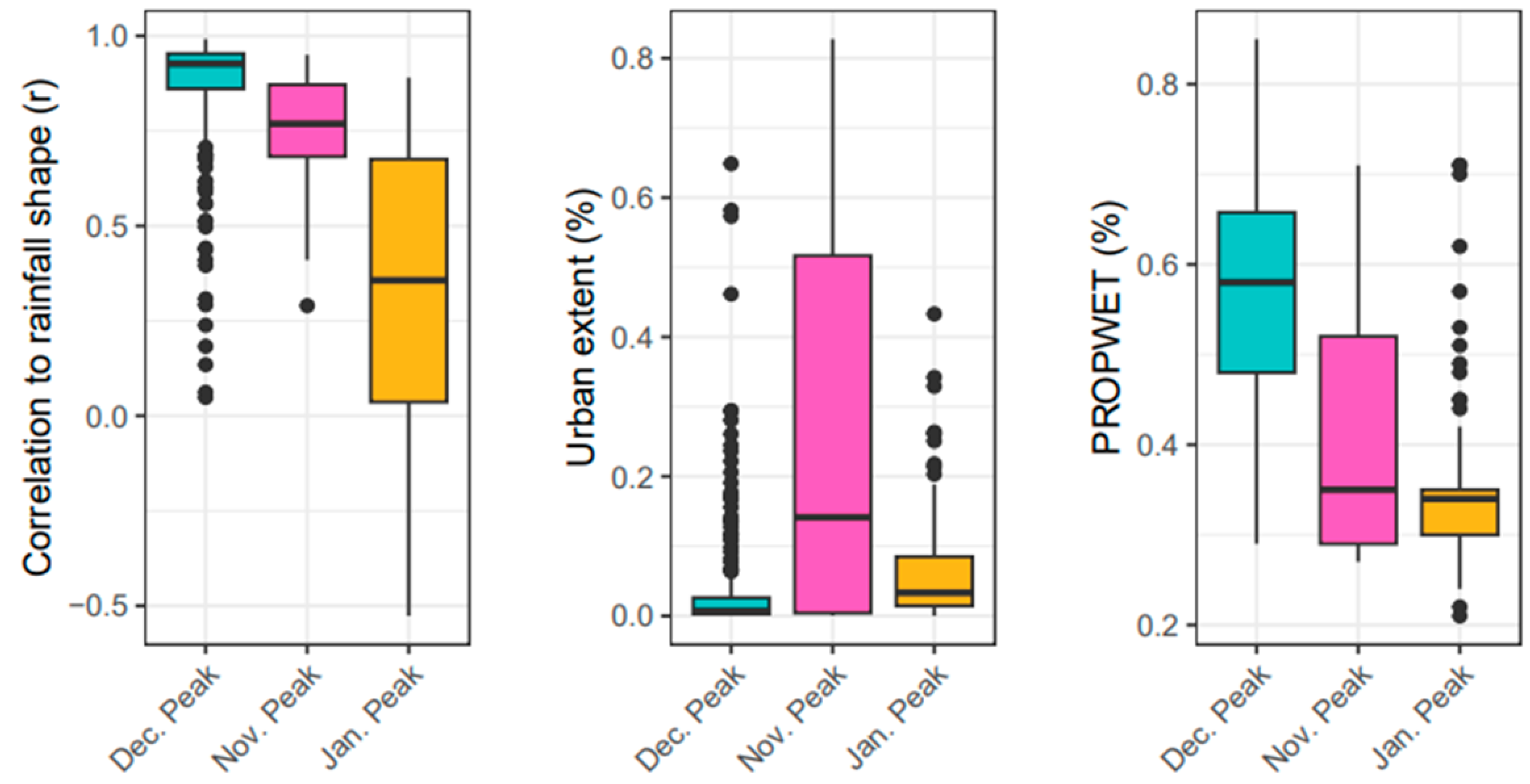
12]. Although Great Britain does not span a wide range of climates, catchment size was still found to characterise flashiness in the north and west from the random forest analysis, whilst being far less critical in other regions. In the north and west, where flood attenuation by soils is less prominent due to a higher PROPWET, catchment size likely plays a larger role in reducing flashiness. A longer drainage path is expected to improve the chances for rainfall to be either intercepted or stored in soil, preventing it from increasing river flow. Larger catchment sizes may reduce flashiness across the entirety of Great Britain, although their effect may be eclipsed by other regional modes of flood attenuation, such as soil moisture availability in the south-east. This relationship between catchment size and flashiness is expected to be stronger when considering smaller time intervals in the
calculation.
4.1.3. Spatial Patterns: Relationship to Urban Areas
Higher flashiness has been observed around major cities in the Midwest, attributed to the increase in impervious cover (Baker). This study finds a similar trend, where the Nov. Peak region captures a large number of urban catchments with increased flashiness. Yet, importantly, this finding relates mainly to the urban area of London, meaning the extracted relationship is skewed toward one urban region. Additionally, with London being underlain by largely impermeable soils [
32], soil dynamics in the area likely conflate this perceived relationship between urban area and flashiness. Besides impervious cover, important factors within urban areas [
34] that impact flashiness also include their location within the catchment [
35], as well as the drainage systems employed [
2], therefore considering merely the proportion of urban area results in an incomplete picture. In order to disentangle these metrics, as well as their implications in temporal analysis, a study of flashiness focusing solely on urban catchments in Great Britain is required, with additional catchment features.
4.2. Trends and Breakpoints: Relationship to UK Hydro-Meterological Patterns
When considering the overall spatial patterns of breakpoints and trends in flashiness, an upward shift was found in the north and south-west of Great Britain. Interestingly, this agrees with regions of observed increases in high flows (Q5) [
35] in an analysis of near-natural catchments, between 1969 and 2008. Similarly in an analysis which investigated the magnitude and frequency of both droughts and floods across Great Britain, hotspots of rapid change were identified in Scotland, and along the west coast of England and Wales [
36]. The results from this study further expand upon which regions are of greatest concern when it comes to hydro-hazards, with flashiness capturing both increases in magnitude and frequency of peak flows. When considering the timing of breakpoints in the 1970–2020 period, these were detected largely between 1987 and 2000. During this period, an increase in rainfall across the UK, as well as a steady increase in mean temperature, has been observed [
37], with both being potential drivers for increasing and decreasing flashiness, respectively. Specific hydrological events were attributed to changes observed in this paper, e.g., the hydrological drought in 2010–2012.
Based on the random forest analysis, mean rainfall did demonstrate some importance in increasing flashiness in the north and west (“Dec. Peak region”), and indeed the region is characterised by a higher PROPWET, impeding rainwater storage. In this region, Slingo [
38] notes that climate change has already triggered significant increases in mean rainfall. The analysis of seasonal patterns in flashiness across Great Britain suggests an oscillation between autumn, winter and spring peaks, with no clear temporal trends observed. Although mean rainfall in the UK has seen a more notable increase in winter [
37] and winter rainfall intensity is projected to increase [
38], this is not yet reflected in the timing of flashy events.
4.3. Implications in River Management
There is nothing inherently problematic with an undisturbed flashy river, and indeed the environment has adjusted to accommodate these. Freshwater ecosystems, however, are vulnerable to flow regime changes [
9], and with over half of the 208 rivers considered displaying significant temporal changes (including breakpoints and/or trends), this is cause for concern. Given that flashiness has also been used to estimate diffuse source pollution [
7,
8], the widespread increase in flashiness on the Scottish east coast could be detrimental to river and coastal health, with run-off emanating from agricultural areas, plantations or industrial areas, particularly when considering emerging contaminant movement through catchments.
Through the random forest analysis, this study demonstrated that reservoirs and lakes have a significant impact on river flashiness in the north and west of Great Britain. When it comes to artificial reservoirs, some level of natural flashiness should be preserved. Importantly, stations affected by artificial reservoirs may experience significant sub-daily variations in streamflow [
39], and different time intervals should be considered when assessing their outflows. The strong relationship between BFIHOST and
suggests that much like the BFI, the
could be predicted for ungauged catchments based on a multiple linear regression of HOST classes. This is especially relevant in the south-east (“Jan. Peak region”), which had the strongest link to the BFIHOST. However, considering the non-stationarity in flashiness, the variable weights would likely need recalibration at regular intervals. In the same vein, given the correlation between the
and BFI (r = −0.898) the
could serve as an alternative to the BFI for low flow estimation.
4.4. Limitations of the Study
Within this study, some limitations in the results emerged. The most notable regards the unmonitored locations. Within both time-periods considered, there is a dearth of data available for river catchments on the west coast of Scotland and the Scottish Isles. When using a full 50-year period, much of northern England was also ungauged. Although shorter time periods could be utilised, which would allow for more stations to be utilized, this would limit the validity of the temporal trends and
—a set of potentially anomalous years could be captured and skew the results. Given that the Scottish west coast has already experienced significant increases in mean rainfall [
38], it is speculated that this region would likely demonstrate increases in flashiness similar to the rest of Scotland.
Items on a cluster boundary may potentially be miscategorised, especially when elements do not gravitate around any particular centroid. This was the case for the “Nov. Peak region”, which contained a set of stations that did not fit with other shape regions, and showed a broad range of shapes within their own cluster. Additionally, anomalous stations may not have sufficient quantity to form clusters, despite having distinct qualities. This was apparent for the two-stage clustering of yearly shapes, where numerous outliers were found in summer months, yet these summer peaks were not dominant enough to form a separate cluster. For the random forest analysis, the performance is negatively affected by sample sizes. A low number of stations means that the number of points at the lowest node split becomes significant relative to the total sample size, and thus the final regression has large uncertainty.
Looking at breakpoints and trends in flashiness, these showed significant overlap. In the same vein, similar spatial patterns in breakpoints and trends were found when analysing peak flows in the continental US [
23]. Breakpoints represent a step-change which occurs at a single point in time; by contrast, trends represent a continuous upward or downward motion. Essentially, breakpoints could be dismissed as a one-off event, and efforts to reverse the “jump” in flashiness may be left to future generations. Given the large overlap found between breakpoints and trends, it is stressed that breakpoints must not be dismissed as one-off events, and immediate efforts should be made to reverse these changes in flashiness regardless.
5. Conclusions
This research identified spatial and temporal patterns in river flashiness in Great Britain. An overall west-coast–east-coast gradient was found in flashiness magnitude. However, some outliers were visible, most notably in the Lake District and Greater London, likely influenced by flood attenuation by lakes/reservoirs, clay content and urban areas. By clustering the average flashiness “shapes”, Great Britain can be split into two major flashiness regions—the “Dec. Peak region” (north and west) and the “Jan. Peak region” (south-east)—which operate using distinct hydrological mechanisms. An additional third region was identified including a small set of stations that did not conform with other clusters, yet this region was too small to highlight predictors or patterns in flashiness with certainty.
Using a random forest analysis, the potential predictors for average flashiness were extracted in each region. Overall soil composition played a major role in predicting flashiness across Great Britain, with some additional regional predictors such as FARL and catchment area in the north and west. This reliance on BFIHOST demonstrates the potential of the in being estimated from HOST soil classes, for catchments without any gauge stations. Flashiness displayed some relationship to urban areas, yet with results skewed towards Greater London, these provide an incomplete picture and require further analysis.
Temporally, over half of the 208 stations with a complete 50-year period demonstrated breakpoints and/or trends in yearly flashiness. The regions with increases in flashiness were found to be in the north-east and south-west, with concerning implications in diffuse source pollutant concentrations as well as flood frequency and rapidity. Importantly, some spatial gaps are present, with the west coast of Scotland and the north of England having few stations available for a 50-year analysis, which means their trends are not studied here. To assess how the timing of flashy events has changed over the 50-year period, 10,400 yearly flashiness shapes were clustered. In the major flashiness regions, flashy events oscillated between periods of late-autumn and early-spring peaks in the past 50-years, with no clear trends identified. As expected, flashy events occurred earlier in the north and west, and later in the south-east. However, with summer peaks in flashiness being relatively uncommon, these were not captured in the resulting clusters, and could not be analysed in this study.
Overall, this study outlines the most influential predictors of flashiness in Great Britain and highlights significant temporal changes observed in the past 50 years. It is encouraged that the Richards–Baker flashiness index be considered when preserving natural flow regimes, as it highlights key hydrological processes. Additionally, efforts should be made to maintain biodiversity and river health in locations of significant trends/breakpoints in flashiness, as well as downstream of artificial reservoirs. The methods employed in this paper could be applied to other countries, provided that long-term timeseries gauged flow records are freely available.
Future work in this area could include exploring the influence of climate change on the evolution of patterns through time (
Figure 8,
Figure 9,
Figure 10 and
Figure 11). For example, statistical methods which take a statistical approach to disentangling the climate change signal from the land use change signal in hydrological timeseries and derived metrics [
40] would provide an interesting analysis to inform future water management.


