Article

Investigating Different Interpolation Methods for High-Accuracy VTEC Analysis in Ionospheric Research

Department of Geomatics Engineering, Faculty of Engineering and Natural Sciences, Konya Technical University, Konya 42250, Türkiye
*
Author to whom correspondence should be addressed.
Atmosphere 2024, 15(8), 986; https://doi.org/10.3390/atmos15080986
Submission received: 9 July 2024 / Revised: 5 August 2024 / Accepted: 16 August 2024 / Published: 17 August 2024
(This article belongs to the Special Issue Coupling between Plasmasphere and Upper Atmosphere)

Abstract

:
The dynamic structure of the ionosphere and its changes play an important role in comprehending the natural cycle by linking earth sciences and space sciences. Ionosphere research includes a variety of fields like meteorology, radio wave reflection from the atmosphere, atmospheric anomaly detection, the impact on GNSS (Global Navigation Satellite Systems) signals, the exploration of earthquake precursors, and the formation of the northern lights. To gain further insight into this layer and to monitor variations in the total electron content (TEC), ionospheric maps are created using a variety of data sources, including satellite sensors, GNSS data, and ionosonde data. In these maps, data deficiencies are addressed by using interpolation methods. The objective of this study was to obtain high-accuracy VTEC (Vertical Total Electron Content) information to analyze TEC anomalies as precursors to earthquakes. We propose an innovative approach: employing alternative mathematical surfaces for VTEC calculations, leading to enhanced change analytical interpretation for anomaly detections. Within the scope of the application, the second-degree polynomial method, kriging (point and block model), the radial basis multiquadric, and the thin plate spline (TPS) methods were implemented as interpolation methods. During a 49-day period, the TEC values were computed at three different IGS stations, generating 1176 hourly grids for each interpolation model. As reference data, the ionospheric maps produced by the CODE (Center for Orbit Determination in Europe) Analysis Center were used. This study’s findings showed that, based on statistical values, the TPS model offered more accurate results than other methods. Additionally, it has been observed that the peak values in TEC calculations based on polynomial surfaces are eliminated in TPSs.

1. Introduction

The ionosphere layer, which is a region of Earth’s upper atmosphere, has an important role in the propagation of radio waves, the operation of worldwide communication, geomagnetic storm impact studies, navigation systems, and earthquake precursor studies. Ionospheric studies are critical for understanding the intricate interactions that occur within this atmospheric layer, as well as the variables that influence its fluctuation. The concentration of free electrons along a receiver-satellite signal path, measured as the TEC, is an essential statistic for monitoring ionospheric activity. The introduction of Global Navigation Satellite Systems (GNSS) has provided a dense satellite network for the continuous monitoring of the TEC, resulting in a great contribution to the field of ionospheric research.
Several international organizations and analytical centers, like the International GNSS Service (IGS), the Center for Orbit Determination in Europe (CODE), and the Jet Propulsion Laboratory (JPL) and so on, have an essential part in furthering ionospheric research by producing global ionospheric maps (GIMs). These maps are useful for visualizing the spatial and temporal fluctuations in the total electron content (TEC) across Earth’s ionosphere. These analysis centers use mathematical models that combine data from different GNSS satellites to provide a comprehensive picture of ionospheric electron density distribution. For different studies, GIMs were used as source data for studies or reference data to compare and calculate the accuracies of the studies [1,2,3]. To generate continuous ionospheric maps by estimating values at unsampled locations, different interpolation techniques are implemented. Researchers are executing and improving interpolation algorithms in order to increase the accuracy of global/regional ionospheric maps. The study referenced in [4] applied a kriging interpolation algorithm to improve the global ionospheric maps of UPS (Technical University of Catalonia) produced using GPS measurements. As a result of the study, the RMS (root mean square) of the STEC (slant total electron content) values was improved by 16% over the UPS GIM and by 2% over the IGS GIM. When a comparison was made of the VTEC values retrieved from TOPEX/Poseidon and JASON altimetry data, the RMS improved by 0.3 TECU (6%) and 0.1 TECU (3%), respectively. Ref. [5] produced a regional ionospheric map using un-differenced carrier phase data of multi-GNSS measurements to estimate the TEC values by applying the thin plate spline interpolation method. The RMS values of the produced regional ionospheric map were compared to those of the IGS, UPC, JPL, CODE, and ESA TEC maps and it was shown that for every station and day used, the accuracy of the regional map is higher than the accuracy of the maps of analysis centers. Ref. [6] applied two different weighting algorithms, which are the simple weighting (WS) algorithm using satellite angles for the weighting step, and the modified sine weighting (WMS) algorithm defined by the authors as using both satellite angles and azimuth angles to assess the local solar effect, and three different interpolation algorithms, which are linear, natural break, and nearest neighbor, in three IGS stations located in low-latitude, mid-latitude, and high-latitude zones on the days when space weather conditions were the most disturbed and quietest in 2014. The IGS GIM VTEC values were used as the reference data. As a result of the study, they found that although the WMS slightly outperformed the WS function in terms of the results, there are not appreciable distinctions between the weighting functions. Furthermore, surface interpolation techniques yield more accurate results than simple weighting strategies; yet, at high latitudes, weighting techniques outperform the nearest-neighbor method. And on the most disturbed and quietest days, there is no obvious distinction between the TEC and IGS-VTEC. Ref. [7] conducted research to examine several ionospheric models created by different interpolation techniques (inverse distance weighting, radial basic functions, global and local polynomial interpolation, kriging (ordinary, simple, universal, etc.) that the ArcGIS Geostatistical Analyst toolbox provided. They used GNSS measurements to calculate the TEC values. To compare the models, the indicator of the parametric assessment of the quality of estimation (MPQE) produced by themselves was used. The results of the analysis revealed that the local polynomial interpolation approach produces the fewest mistakes among the subjects. Ref. [8], in order to better understand the consequences of seismic activity on the TEC levels, investigated an earthquake with a magnitude of Mw: 6.8 that occurred in Morocco in 2023. GNSS signals from 11 stations were used to calculate the TEC values, the kriging interpolation method was used for spatial mapping, and the 15-day moving average and standard deviation were used to create limit values for the anomaly graphs. The negative and positive anomalies that occurred were evaluated. In addition, the Dst, Kp, and F10.7 space weather parameters were investigated to find out how space weather conditions affect the TEC values. Finally, InSAR processing was carried out using Sentinel-1 satellite data to track ground changes. The study found a correlation between the abrupt uplift (~15 cm) observed in the InSAR evaluation and positive TEC anomalies 1 week before the earthquake. Ref. [9] investigated the possible TEC precursors associated with the Mexico earthquake (Mw: 7.2) that occurred on 4 April 2021. They used data from 200 CORSs (Continuously Operating Reference Stations) to calculate the TEC fluctuations. It was reported that there was a noticeable negative anomaly two days prior to the earthquake, and that the Kp and Dst space climate indices remained steady throughout the study period. Ref. [10] examined ionospheric disturbances as potential precursors to the 21 May 2021 earthquakes in Yangsbi (Ms: 6.4) and Maduo (Ms: 7.4) in China. To determine GPS TEC anomalies, they employed the sliding quartile approach with data from 113 GPS stations and GIM TEC. To acquire the temporal and spatial distribution of the TEC anomalies, natural neighbor interpolation (NNI) was applied as an interpolation method. After removing the days with high space weather conditions from the anomaly days, they observed that there were TEC anomalies dispersed around the areas of the earthquakes, which may be connected to the earthquakes. According to the study’s findings, the earthquake under investigation had an impact on the ionosphere through the thermal and electric field branches within the structure of the LAIC (Lithosphere–Atmosphere–Ionosphere Coupling) mechanism. Ref. [11] analyzed the potential earthquake precursors in terms of b-value analysis, Poisson probability, and TEC variations for the 2022 Colima/Mexico Earthquake (Mw: 7.7). The study examined 57 CORSs for TEC variations 45 days before the earthquake using GPS-TEC analysis software developed by [12]. Natural neighbor interpolation was utilized for the spatial distribution map. After eliminating the effects of space weather conditions, the analysis found that several negative TEC anomalies with low b-values (averagely 0.87 ± 0.02) appeared before the earthquake, indicating a high earthquake possibility with a Poisson probability of 82%.
Many studies in the literature have utilized variations in the ionosphere as earthquake precursors. To detect ionospheric changes, TEC values are estimated using specific mathematical functions. Additionally, there have continually been numerous studies employing different methodologies to estimate TEC values. It is crucial that the mathematical functions used to calculate and interpret anomalies as earthquake precursors accurately represent the TEC values. The misbehavior of TEC values due to incorrect or incomplete modeling can lead to errors in the interpretation of anomalies. Various interpolation techniques (polynomial, kriging, radial basis functions, natural neighbor, etc.) and methods like ANN (Artificial Neural Network) continue to be carefully examined in the literature for TEC value estimation. In this study, the aim was to see the effects of different interpolation algorithms on the calculation of TEC values and interpretations as earthquake precursors. For this purpose, to calculate the TEC values in the zenith direction of stations, four different interpolation algorithms, which include the second-degree polynomial method, kriging (point and block model), the radial basis multiquadric, and the thin plate spline methods, were implemented on the TEC values produced by GPS (Global Positioning System) data from three IGS stations for every hour of the 49-day period. IONEX (Ionosphere Exchange) files of the CODE Analysis Center were utilized as the reference data and several accuracy metrics were generated to provide a comprehensive comparison. Lastly, using the interpolation method with the best accuracy, anomaly graphs of an example earthquake were generated and compared with the old anomaly graphs from the study in Ref. [13]. Additionally, this reference can provide information regarding the connection between ionospheric anomalies and earthquakes.

2. Materials and Methods

In this study, the earthquake that occurred in Chignik, Alaska/USA, in 2021, with a moment magnitude of Mw: 8.2 and a focal depth of 32.2 was used. Figure 1 displays the study area, and the stations that were evaluated. The radius of the earthquake preparation area was calculated using the Dobrovolsky formula (Rkm = 100.43M) [14] and was found to be 3357.376 km.
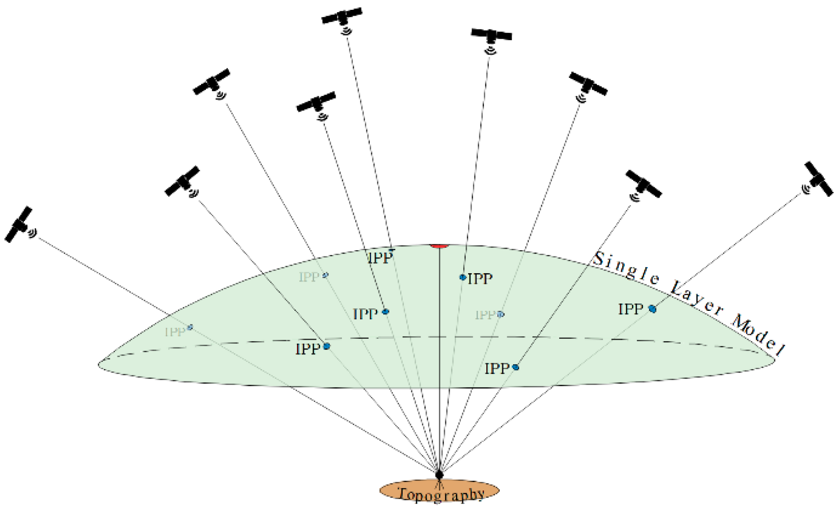
Because of the ionosphere layer’s acceleration and delay effects on GNSS signals, the amount of TEC in the ionosphere can be calculated. Observation data from three IGS stations (WHIT, DRAO, MKEA), satellite ephemeris data, and ionospheric data from the CODE Analysis Center were downloaded from the NASA/CDDIS (National Aeronautics and Space Administration/Crustal Dynamics Data Information System) center [15]. The TEC values of IPPs (Ionospheric Piercing Points) were calculated using smoothed code measurements of GPS observations. In Figure 2, an instance demonstration of IPPs is given.
The general equation of the GNSS code observation is given in Equation (1).
P ¯ F = ρ F + c Δ t r Δ t s + T + I F + c D C B s + D C B r + α
where P ¯ F is code observation (F = 1, 2), ρ F is the geometric distance between the satellite and receiver, c is the velocity of the light in vacuum, Δ t r is the receiver clock error, Δ t s is the satellite clock error, T is the tropospheric effect, I F is the ionospheric effect. The differential code biases of the satellite and the receiver are denoted by DCBs and DCBr, respectively. The relevant DCB values were obtained from IONEX files from the CODE Analysis Center. Lastly, α   is the state noise of signal.
Code measurements were smoothed using the RNXSMT program in Bernese v5.4 software to remove outliers and cycle slips [16]. Calculations of smoothed code measurements are given in Equation (2).
P ~ 1 t = ϕ 1 t + P ¯ 1 ϕ ¯ 1 + 2 f 2 2 f 1 2 f 2 2 ϕ 1 t ϕ ¯ 1 ϕ 2 t ϕ ¯ 2   P ~ 2 t = ϕ 2 t + P ¯ 2 ϕ ¯ 2 + 2 f 1 2 f 1 2 f 2 2 ϕ 1 t ϕ ¯ 1 ϕ 2 t ϕ ¯ 2
where P ~ F t is the smoothed code measurement (epoch t and frequency F = 1, 2). ϕ F t is the carrier phase measurement (epoch t and frequency F = 1, 2) and P ¯ F ϕ ¯ F is the mean difference between all the accepted code and phase measurements in the current observation arc on frequency F = 1, 2 [16]. After the smoothing step, frequency-independent effects will be eliminated by creating geometry-free combinations (Equation (3)).
P 4 , r s = P ~ 1 P ~ 2 = 40.3 1 / f 1 2 1 / f 2 2 S T E C r s + D C B s + D C B r
STEC values along the receiver-to-satellite path can be computed using Equation (4):
S T E C r s = 1 40.3 f 1 2 f 2 2 f 2 2 f 1 2 P 4 , r s c D C B s + D C B r
S T E C r s is the slant total electron content, f1 and f2 refer to the signal frequencies of the carrier wave, P 4 , r s is the difference in the smoothed codes between P ~ 1 and P ~ 2 , c is the velocity of light. After calculation of the STEC values of IPPs, various interpolation methods were applied to determine the STEC values in the receiver’s zenith direction. For the STEC value in the zenith direction of a station, only STEC values of IPPs calculated from that station and satellites were used as reference points in the interpolations. IONEX files from the CODE Analysis Center were used to investigate the accuracies of calculated STECs. STEC values of the station’s zenith direction were obtained using the grid interpolation method as a suggestion from Ref. [17] in the IONEX: Ionosphere Map Exchange Format Version 1.1 file. As accuracy metrics, standard deviation, RMSE, R2, d (Index of Agreement), Pearson’s correlation coefficient, c (the confidence index), and KGE (Kling–Gupta efficiency) were used. The best interpolation model for this study was selected and it was executed in the following steps.
To calculate the VTEC of IPPs from STEC values, the modified single layer model (MSLM) mapping function M(z) was used (Equation (5)):
V T E C = S T E C M z , M z = 1 1 sin 2 z , z = sin 1 R e R e + H sin α S L M z
where R e is the radius of Earth (6371 km), H is the orthometric height of the single layer model for the ionosphere (450 km determined by CODE Analysis Center), α S L M is the geocentric angle in the single layer model of the ionosphere, and z states the zenith angle of the relevant satellite. Following the calculation of the VTEC values of the ionospheric piercing points, the selected interpolation method was applied to determine the VTEC value in the receiver’s zenith direction. As a final step, anomaly graphs were generated by using the moving median method on the interquartile range. In this method, using the VTEC values from the first 15 days of the data range, the limit boundaries for the 16th day were determined. Then, the limit boundaries for the 17th day were determined using the VTEC values between the 2nd day and the 16th day. The process continued in this way over a moving median with a sliding window. Since the boundary values are determined based on the VTECs obtained from interpolation methods, each method has its own specific boundaries which are created and evaluated accordingly. The limit boundaries set by Ref. [18] were implemented (Equation (6)), resulting in a probability of approximately 65% for a new TEC value between LB and UB. Values that exceeded the limitations are displayed as anomalies in the graphs.
U B = M + 1.5 U Q M L B = M 1.5 M L Q
where UB refers to upper bound, M is median value, LB is lower bound, UQ and LQ are upper and lower quartiles, respectively.

2.1. Interpolation Methods

Interpolation is an important mathematical technique that plays a fundamental role in data analysis, modeling, and prediction processes in engineering fields. This method is used to estimate the values of a continuous function with information extracted from incomplete or limited datasets. Interpolation comes with a wide range of applications; it is used in geodetic applications, geographic information systems, image processing, engineering designs, and many other areas. In this section, it will focus specifically on interpolation methods such as polynomial interpolation, kriging interpolation, and radial basis functions. The mathematical foundations and brief introductions of these interpolation methods used within the scope of the application will be given in this section.
  • Polynomial Interpolation Method
Polynomial interpolation is an advanced interpolation technique that strives to identify the most suitable polynomial function for the given data [19]. For this study, polynomial surface coefficients were estimated using TEC values and locations using IPPs by the least squares method. The receiver’s latitude and longitude were inserted into the equation, and the TEC value in the zenith direction of the receiver was computed [13].
T E C φ I P P , λ I P P = a 0 + a 1 φ I P P + a 2 λ I P P + a 3 φ I P P 2 + a 4 φ I P P λ I P P + a 5 λ I P P 2
φ I P P = Latitude of the ionosphere piercing point in the solar fixed reference system.
λ I P P = Longitude of the ionosphere piercing point in the solar fixed reference system.
a i = Polynomial surface coefficients.
The least squares method was used to derive the model coefficients. Then, using the latitude and longitude of the station in the solar fixed reference system, and model coefficients and the TEC values of the zenith direction of the station were calculated. The method’s phases are given in Equation (8), where A is the coefficient matrix, l is the measurement vector, and x is the unknown vector.
A = 1 φ I P P , 1 λ I P P . 1 φ I P P , 1 2 φ I P P , 1 λ I P P , 1 λ I P P , 1 2 1 φ I P P , 2 λ I P P . 2 φ I P P , 2 2 φ I P P , 2 λ I P P , 2 λ I P P , 2 2 1 φ I P P , 3 λ I P P . 2 φ I P P , 3 2 φ I P P , 3 λ I P P , 3 λ I P P , 3 2 1 φ I P P , n λ I P P . n φ I P P , n 2 φ I P P , n λ I P P , n λ I P P , n 2 ,   l = T E C 1 T E C 2 T E C 3 T E C n ,   x = a 0 a 1 a 2 a 3 a 4 a 5
x = A T A 1 ( A T l )
  • Kriging Interpolation Method
Kriging is a geostatistics interpolation technique that is extensively applied across multiple fields, particularly in earth sciences and geographic information systems (GISs). Kriging interpolation is a reliable method for estimating VTEC values at unknown locations, resulting in a continuous model of the ionosphere while minimizing the estimated variance [8]. In order to perform kriging, a variogram must be fit to determine the spatial covariance structure of the reference points. Then, using weights obtained from this covariance structure, values for new points or blocks belonging to the spatial field are interpolated. The general equation of the kriging method is as follows:
Z ^ s 0 = i = 1 N λ i Z s i
Z(si) = the value that was measured at the i. location.
λi = an unknown weight at the i. location for the observed value.
s0 = the prediction location.
N = the total number of measurements.
Point kriging (KrigingP) and block kriging (KrigingB) both provide an interpolated grid. KrigingP calculates the values of points at grid nodes. Through the use of KrigingB, the average value of the rectangular blocks that are centered around the grid nodes is estimated. A grid cell’s size and shape correspond to the blocks. KrigingB creates smoother contours since it estimates a block’s average value. Moreover, KrigingB is not an ideal interpolator because it does not estimate the value at a specific point. This means that the KrigingB estimate for a grid node does not precisely replicate the observed value, even if the observed value occurs exactly on that node [20,21,22,23,24].
  • Radial Basis Function
The radial basis function (RBF) method is a widely used mathematical technique for solving problems in geophysics, mapping, topography, hydrology, and particularly in interpolation and machine learning. RBFs are particularly notable for their flexibility, ease of use, and accuracy when applied to sparse, multidimensional datasets. An RBF-based interpolation model utilizes fundamental functions based on the radial distances between the interpolation point and all other points in the dataset. Numerous studies have shown that accurate results can be obtained using RBF methods, even when the data are not uniformly distributed across the area or region. This important feature makes RBFs particularly ideal for sparse data. Radial-based algorithms are among the most effective for correcting local distortions [5,25,26,27,28,29,30,31]. Therefore, in this study, we decided that it is appropriate to use RBF-based algorithms such as multiquadric (MQ) and thin plate spline (TPS).
The multiquadric method (MQ) is one of the radial basis algorithms. For each given reference point, a function in the form of B i x , y is selected using this procedure. The function f x , y = i = 1 n c i B i x , y is utilized to compute the coefficients c i , which provides the interpolation value. The most commonly utilized function type as a B i x , y function is a single-variable radial function. To achieve this, a radial function in the form B i x , y = B h i is employed, where h i represents the distance between two points [24,32]. The accuracy of the multiquadric method is determined by a user-specified shape parameter R2 [33]. The interpolation’s smoothness can be impacted by the shape parameter R2, which is most frequently chosen based on the specifics of the given situation.
h i = x x i 2 + y y i 2
B h i = h i 2 + R 2
z = i = 1 n c i B h i
where h i   represents the Euclidean distance between the data point and the node, R 2 is the user-specified shaping factor, z is the multiquadric surface. There are several proposals in the literature about the value that the R 2 parameter can assume [20,34,35,36]. Given n data points, if the MQ basis functions are assumed to pass through these points, meaning they are equal to the measured or known values ( z j ), the following equation can be obtained:
z j = i = 1 n c i B h i j     j = 1,2 , , n
h i j = x j x i 2 + y j y i 2
B h i j = h i j 2 + R 2
h i j defines the Euclidean distance between two points, specifically the distance from the j-th interpolation point to the i-th data point. B h i j represents the multiquadric radial basis function, c i are the unknown coefficients, and z j denotes the measured values at the j-th data point. When these equations are converted into a linear system, the following is obtained:
Ψ c = z
The solution in matrix form is given by Equation (17):
c = Ψ T Ψ 1 Ψ T z
Here, Ψ n x n is the basis function matrix, c 1 x n is the vector of unknown coefficients, and z 1 x n is the measurement vector, which can be defined as follows:
Ψ n x n = B h 11 B h 12 B h 13 B h 1 n B h 21 B h 22 B h 23 B h 2 n B h 31 B h 32 B h 33 B h 3 n B h n 1 B h n 2 B h n 3 B h n n , c 1 x n = c 1 c 2 c 3 c n , z 1 x n = z 1 z 2 z 3 z n
Once the unknown coefficients are obtained, the estimated values ( z ^ j ) for the interpolation points are calculated using Equation (19).
z ^ j = i = 1 n c i B h i j
Thin plate splines (TPSs) belong to the class of radial basis function (RBF) interpolation algorithms, just like the MQ method. This method’s surface is softer than the multiquadric surface and responds better to the original surface [32,37]. The TPS approach is another mathematical methodology used for interpolation and approximation, particularly in computer graphics, image processing, and surface modeling. The solution for the TPS method is similar to that of the MQ method. The primary difference lies in the basis function used. In the TPS method, instead of the basis function used in the MQ method (Equation (15)), the basis function specified in Equation (20) is used. Essentially, apart from the basis function, the solution for the TPS method is obtained in a manner similar to the MQ method, and the values at the interpolation points are calculated. For more detailed information on the interpolation methods, refer to sources [5,6,7,25,26,27,28,29,30,31,32,33,34,35,36,37].
B h i j = h i j 2 + R 2 l n h i j 2 + R 2

2.2. Evaluation Parameters

In this study, various evaluation metrics were employed to elucidate the relationship between predicted and reference values and to ascertain the most suitable model. Residuals, commonly utilized in many studies, such as minimum, maximum, standard deviation (std), and root mean squared error (RMSE), were considered for model comparison. Additionally, we explored the appropriateness of models by incorporating metrics like the coefficient of determination (R2), the Index of Agreement (IA), the confidence index (c), the Pearson correlation coefficient (R), and the Kling–Gupta efficiency (KGE).
Standard deviation (std) is a statistical term that gauges the dispersion of values around the average (or mean) in a dataset. It measures how far individual data points deviate from the central value. A low standard deviation suggests that the data points are closely clustered around the average, while a high standard deviation indicates a more widespread distribution. Standard deviation is frequently employed to assess the variability and spread of a dataset [38]. The standard deviation value is calculated with Equation (21).
s t d = i = 1 n x i x ¯ 2 n 1
Root mean squared error (RMSE) is a statistical metric that quantifies the extent to which a model’s predictions differ from the reference values. A low RMSE suggests close agreement between the model’s predictions and the reference values, while a high RMSE indicates a larger degree of deviation. RMSE is calculated using Equation (22), where the specific formula is used to measure the average magnitude of these prediction errors.
R M S E = i = 1 n x i y i 2 n
The Pearson correlation coefficient (R) is a statistical metric that quantifies the linear relationship between two variables, taking a value between −1 and 1. This coefficient is widely used to evaluate both the magnitude and direction of the linear relationship between variables. A positive correlation signifies that an increase in one variable corresponds to an increase in the other, while a negative correlation implies an inverse relationship. A correlation close to 0 signifies the absence of a linear relationship between the variables [39]. The R-value can be calculated with Equation (23).
R = i = 1 n x i x ¯ y i y ¯ i = 1 n x i x ¯ 2 i = 1 n y i y ¯ 2 , 1 R 1
The Index of Agreement (IA) [40] serves as a metric to assess the likeness between the model’s predicted values and the reference values. Ranging between 0 and 1, the IA value indicates the model’s success. A value approaching 1 signifies a higher resemblance between the model’s predictions and the observed values [41]. The calculation of the IA value is performed using Equation (24).
I A = 1 i = 1 n x i y i 2 i = 1 n y i x ¯ + x i x ¯ 2 , 0 I A 1
The confidence index (c) serves as a comprehensive metric, amalgamating both random and systematic errors with equal importance, thereby providing a holistic quantification of model error. In Equation (25), the confidence index is calculated by multiplying the Index of Agreement (IA) with the square root of the coefficient of determination (R2). This formula considers the agreement (Index of Agreement) between the reference and predicted values as well as the explanatory power of the model (coefficient of determination). Consequently, higher confidence index values indicate a more reliable model performance. In practical terms, interpreting the c is based on predefined performance criteria, ranging from “Best” to “Worst”. This categorization allows for a qualitative assessment of models, offering valuable insights into their overall reliability. Notably, if the c exceeds 0.85, it signifies the model’s exceptional performance [42].
c = I A   R 2
The Kling–Gupta efficiency (KGE) assesses the alignment between model predictions and reference values, taking into account the mean, standard deviation, and correlation coefficient. The calculation is defined by Equation (26). A KGE value approaching 1 shows a superior fit of the model predictions to the reference values [41,43,44].
K G E = 1 R 1 2 + s y s x 1 2 + y ¯ x ¯ 1 2
where x is the reference value, y is the prediction value, x ¯ is the average reference value, y ¯ is the average prediction value, s x is the standard deviation of reference value, s y is the standard deviation of prediction value, and n is the number of reference values.

3. Results and Discussion

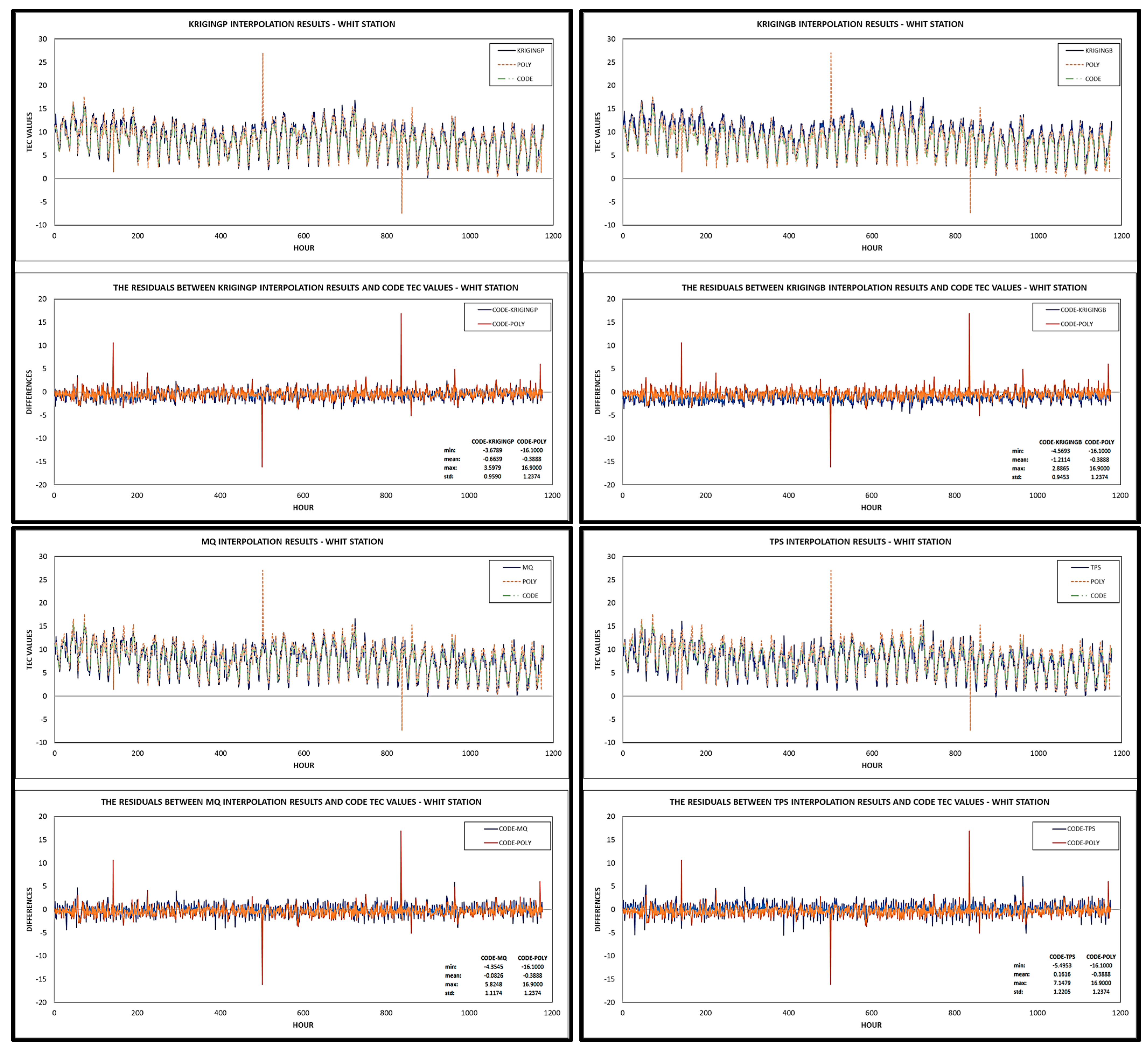
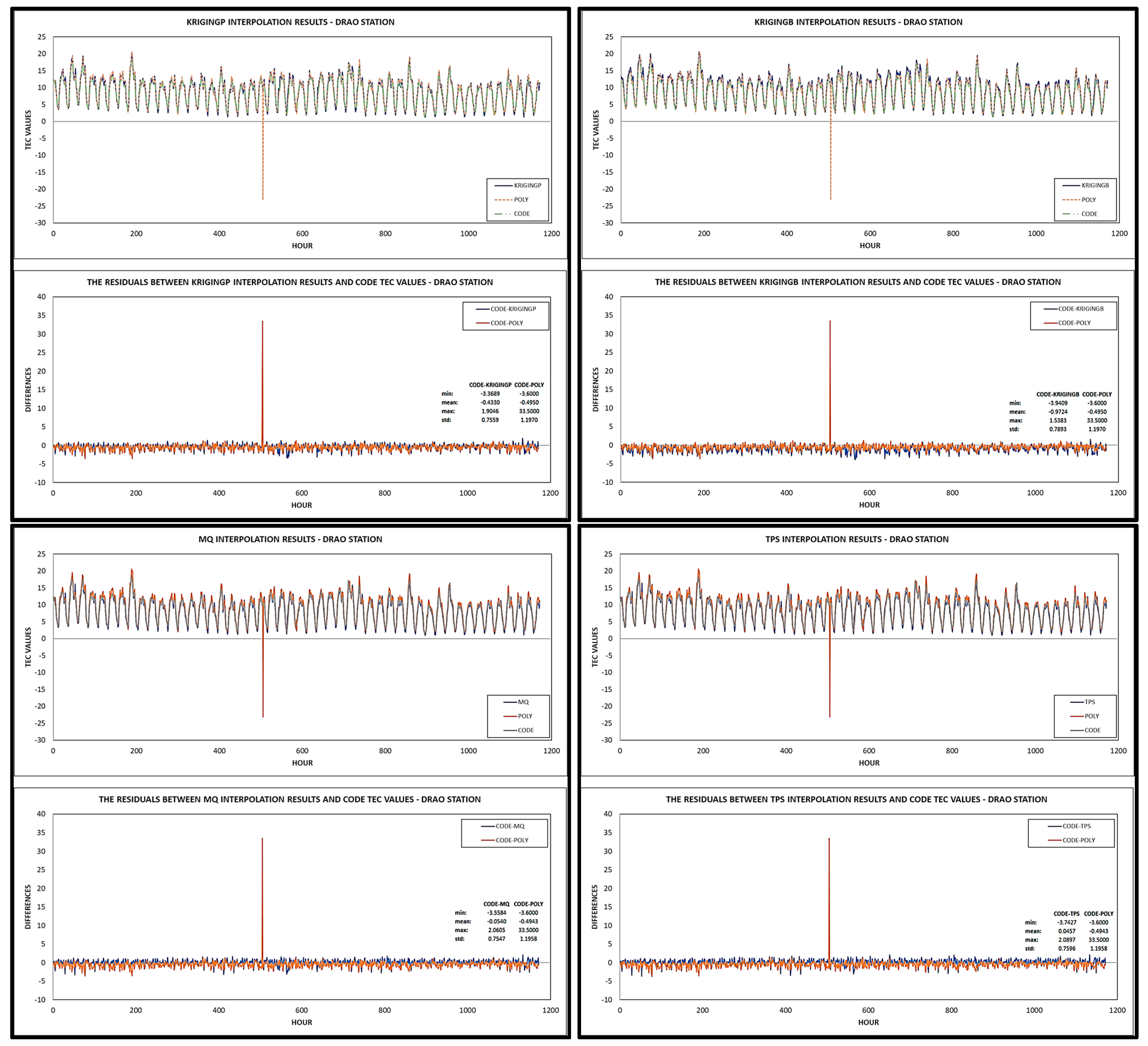
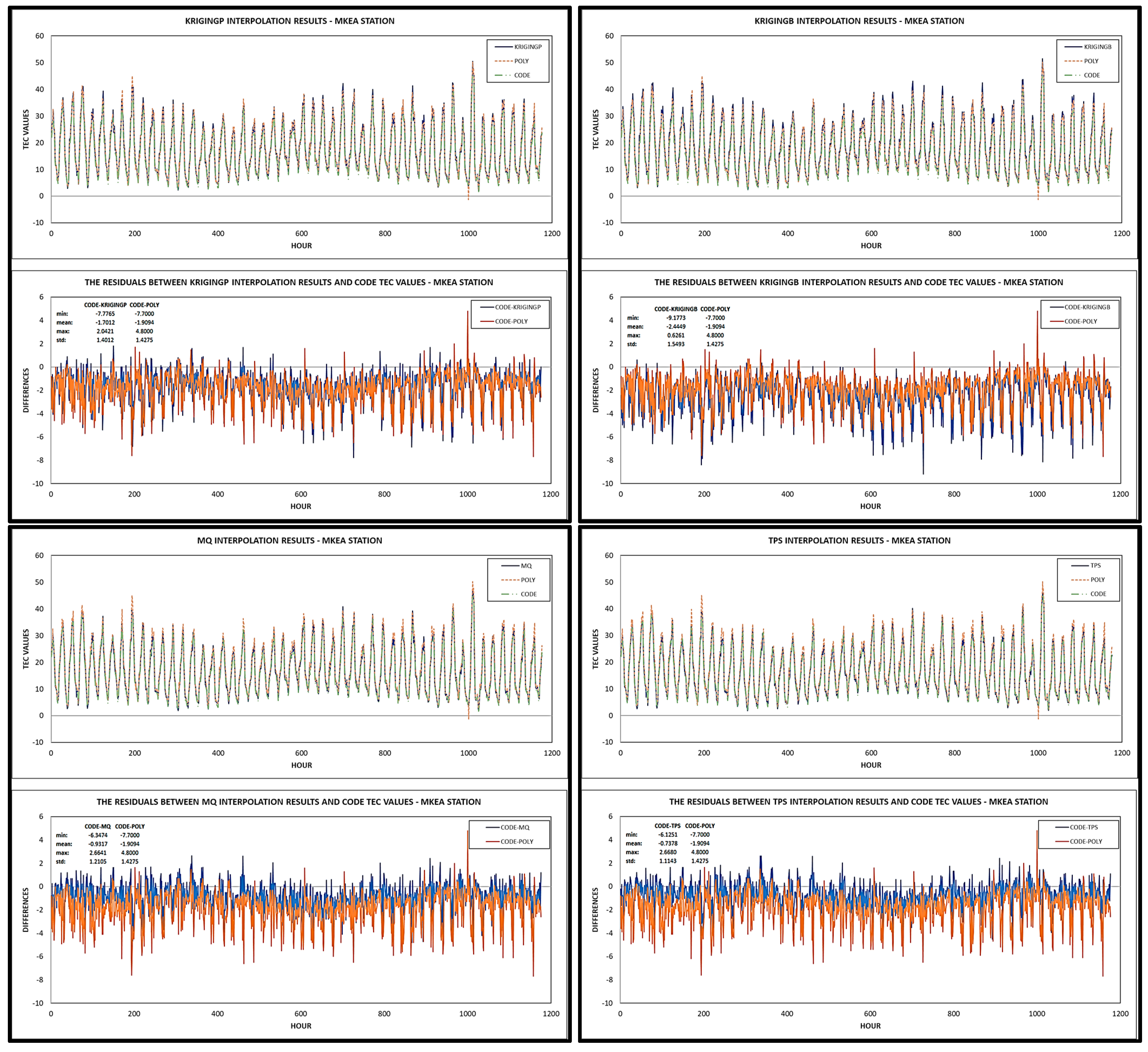
STEC readings in the receiver zenith direction were obtained using all the interpolation procedures. Interpolation methods, including the second-degree polynomial approach, KrigingP, KrigingB, MQ, and TPS, were implemented in the application’s scope. STEC values were generated at three IGS stations (WHIT, DRAO, MKEA) over 49 days, resulting in 1176 hourly grids for each interpolation model. The STEC values from the IONEX file from the CODE Analysis Center were utilized for a comparison. The interpolation results for each method were obtained by computing differences from the IONEX file. Additionally, the performance of the alternative methods was compared to that of the second-degree polynomial surface—a widely used approach in the literature for estimating STEC values. Figure 3, Figure 4 and Figure 5 illustrate comparison graphs for the WHIT, DRAO, and MKEA stations.
When examining Figure 3, Figure 4 and Figure 5, a particularly significant result stands out. As previously mentioned, a second-degree polynomial method is generally used for VTEC estimations in the literature. When the results obtained from this method are examined, a striking outcome is observed with the detection of abrupt jumps. These jumps, especially seen at the WHIT and DRAO stations located in the earthquake-affected area and at different latitudes, clearly indicate that they can lead to negative consequences in the detection of anomalies as earthquake precursors and result in misinterpretations. This is because the UB and LB values used in anomaly detection are calculated by deriving from these values. If there are VTEC values exceeding the UB or LB values, they are considered significant anomalies. When examining the polynomial results at the WHIT station, six sudden jumps are detected, whereas these jumps are eliminated in the results obtained from other methods. Similarly, it is observed that one jump is eliminated at the DRAO station. The last inspection station, MKEA, is a station located slightly outside the earthquake-affected area. When examining the results for this station, it is found that there are no noticeable sudden jumps, but larger difference values are obtained compared to the other stations. Specific comparative values for the differences for all the stations are presented in Table 1, and the histogram plots are shown in Figure 6, Figure 7 and Figure 8.
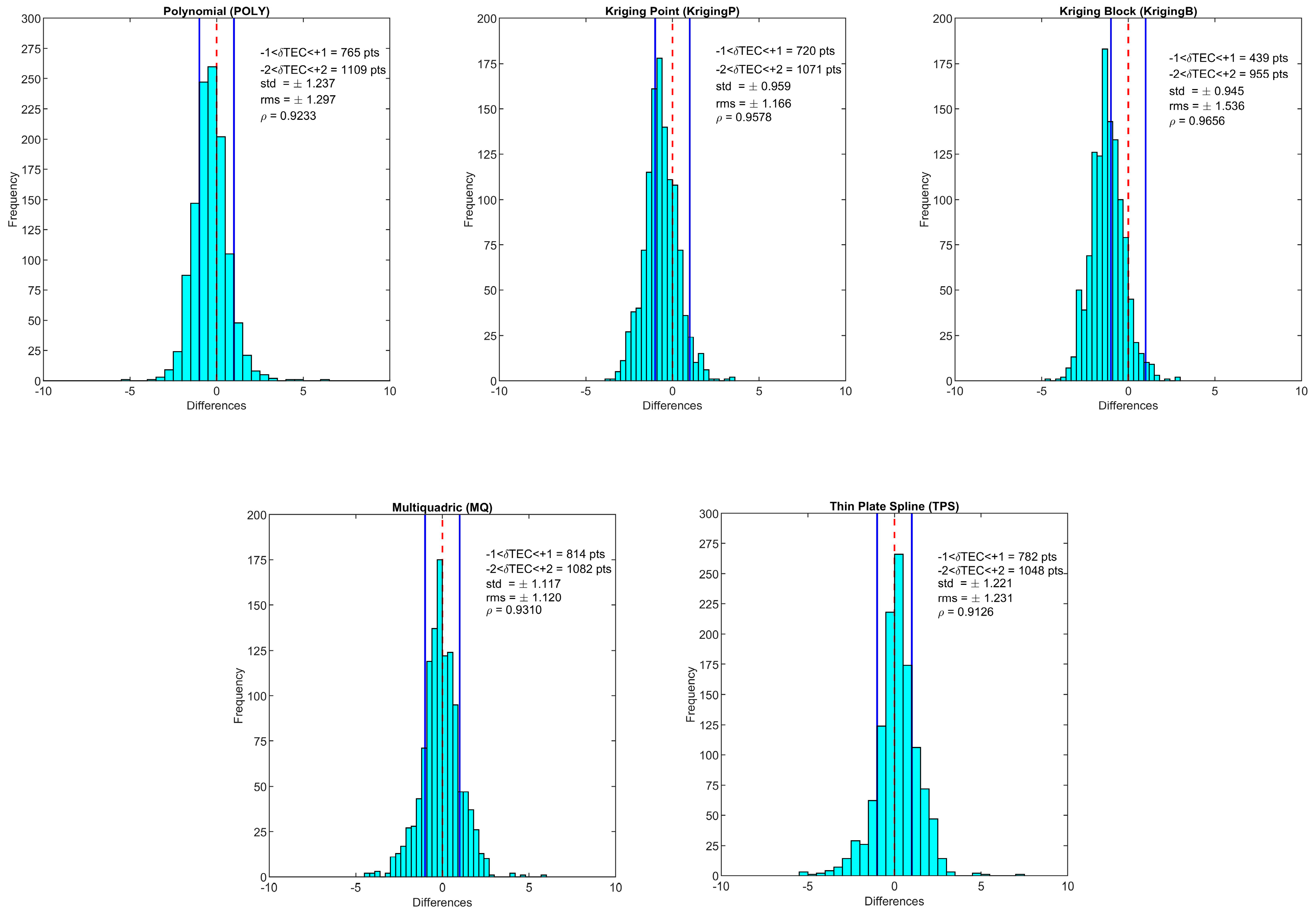
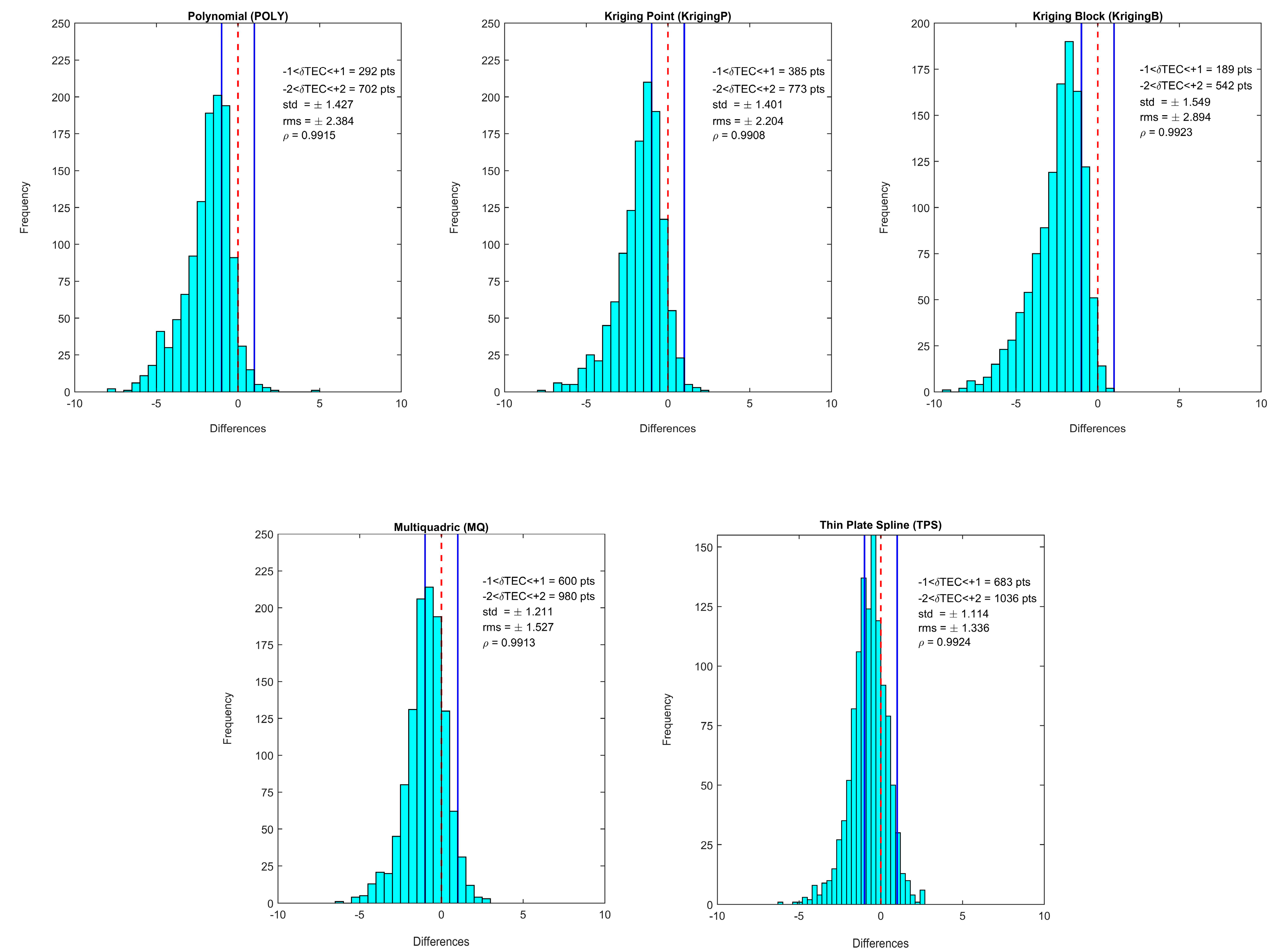
When examining Table 1, it is seen that the results are analyzed with different evaluation criteria. The TEC values obtained from CODE are used as reference data here. Statistical values are calculated by taking the differences in the values obtained from interpolation from the reference values, and the performance of the interpolation methods is presented. In addition, histogram plots are used to provide a better understanding of the differences between the values calculated using the interpolation methods and the actual values (Figure 6, Figure 7 and Figure 8). Some boundary values are added to the histogram plots to observe the distribution of the calculated differences. In the figures, the zero line is shown in red, and the distribution line in the range of (−1 TEC) − (+1 TEC) is shown in blue. Additionally, the number of data points within the boundary values is included in the upper right part of the graphs, along with some statistical information.
Based on these findings, it can be said that the KrigingB and MQ methods stand out with three criteria for evaluation metrics at the WHIT station. However, when a detailed examination is made, it is seen that the std value for the KrigingB method is 0.945, the RMSE value is 1.536, and the KGE value is 0.779, whereas for the MQ method, they are calculated as 1.117, 1.120, and 0.856, respectively. Although the KrigingB model appears better in terms of the std, it has given worse results than the MQ method in terms of the RMSE and KGE. The main reason for this is the distribution of differences. When examining Figure 6, it is clearly seen that the results obtained from the KrigingB method are negatively skewed compared to the expected value. While the standard deviation shows the distribution of values around the mean in a dataset, the RMSE value is a statistical measure that indicates how different the predictions of a model are from the reference values. Therefore, it is important to obtain and interpret both values in such applications. Additionally, in Figure 6, while the number of data points within the range of −2 to +2 for the KrigingB method is found to be 955, it is obtained as 1082 for the MQ method. Similarly, when examining the number of data points within the range of −1 to +1, it is seen that 439 data points fall into this range for the KrigingB method, while 814 data points do so for the MQ method. Therefore, it can be said that the MQ method is better in terms of the distribution of differences, followed closely by the TPS method. One of the other evaluation criteria, IA, is a measure that evaluates the similarity between the predicted values and the reference values, while the KGE criterion evaluates the agreement between the predicted values and the reference values by using the mean, standard deviation, and correlation coefficient. When examining the WHIT station results with these criteria, it is seen that the MQ and TPS methods provide the highest values.
If the other two stations, DRAO and MKEA, are evaluated similarly, the following results are obtained. From Table 1, it is seen that the MQ method stands out for the DRAO station in terms of the std, RMSE, IA, and c, while the results obtained from the TPS method are very close to these values, and especially in terms of the IA and KGE values, the TPS method is in first place. When examining Figure 7, it is found that the number of data points within the range of −2 to +2 for the MQ method is 1140, while it is obtained as 1145 for the TPS method. Similarly, when examining the number of data points within the range of −1 to +1, it is seen that 992 data points fall into this range for both the MQ and TPS methods. This means that the difference values obtained in the remaining 31 epochs for the TPS method are slightly higher than those obtained for the MQ method. However, it would not be wrong to say that both methods give very close results in terms of the distribution. When examining Table 1 for the last station, MKEA, it is clearly seen that the TPS method provides better results in all criteria. When examining the histogram graphs of the differences in Figure 8, it can be said that the TPS method stands out, followed closely by the MQ method.
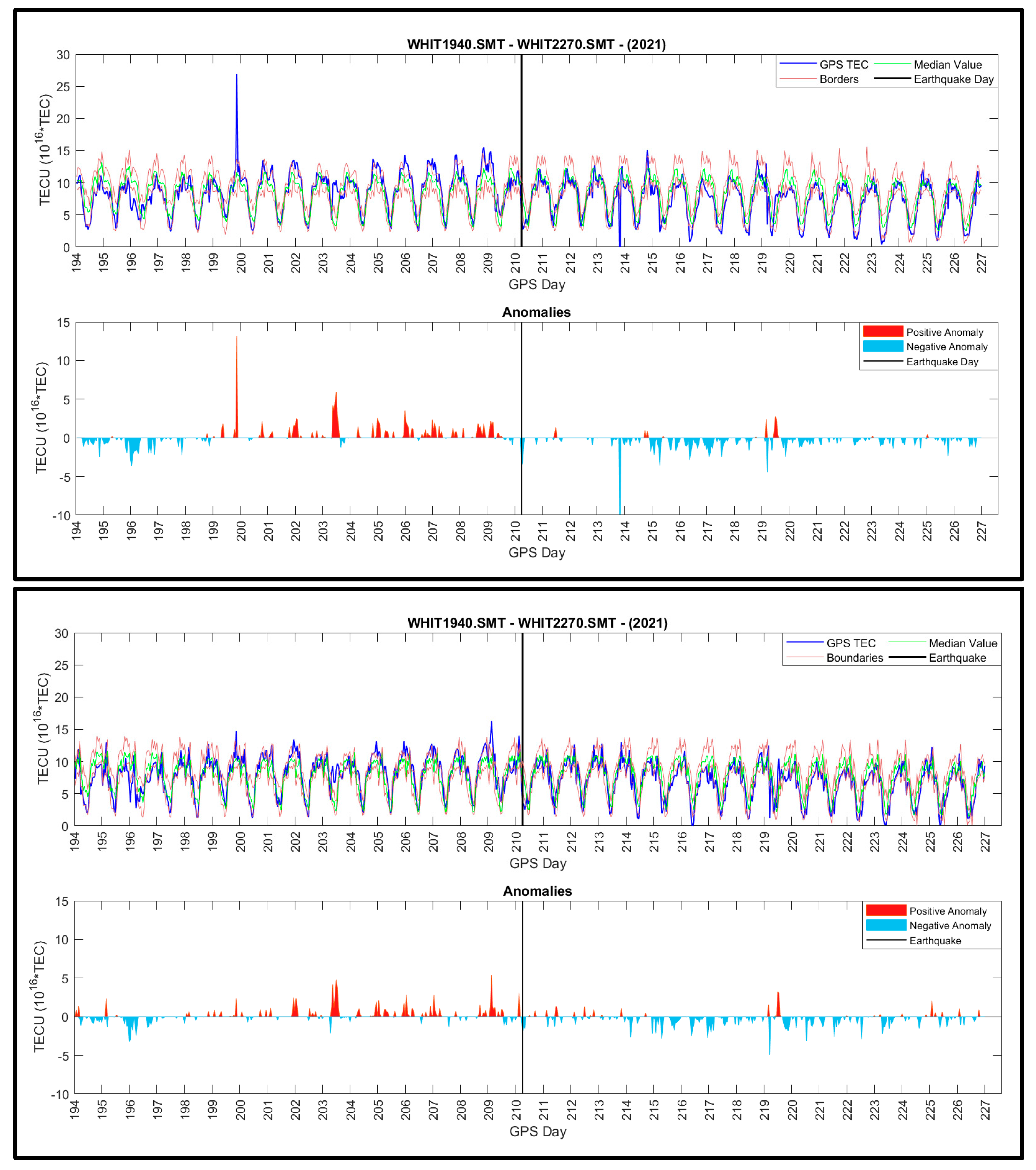
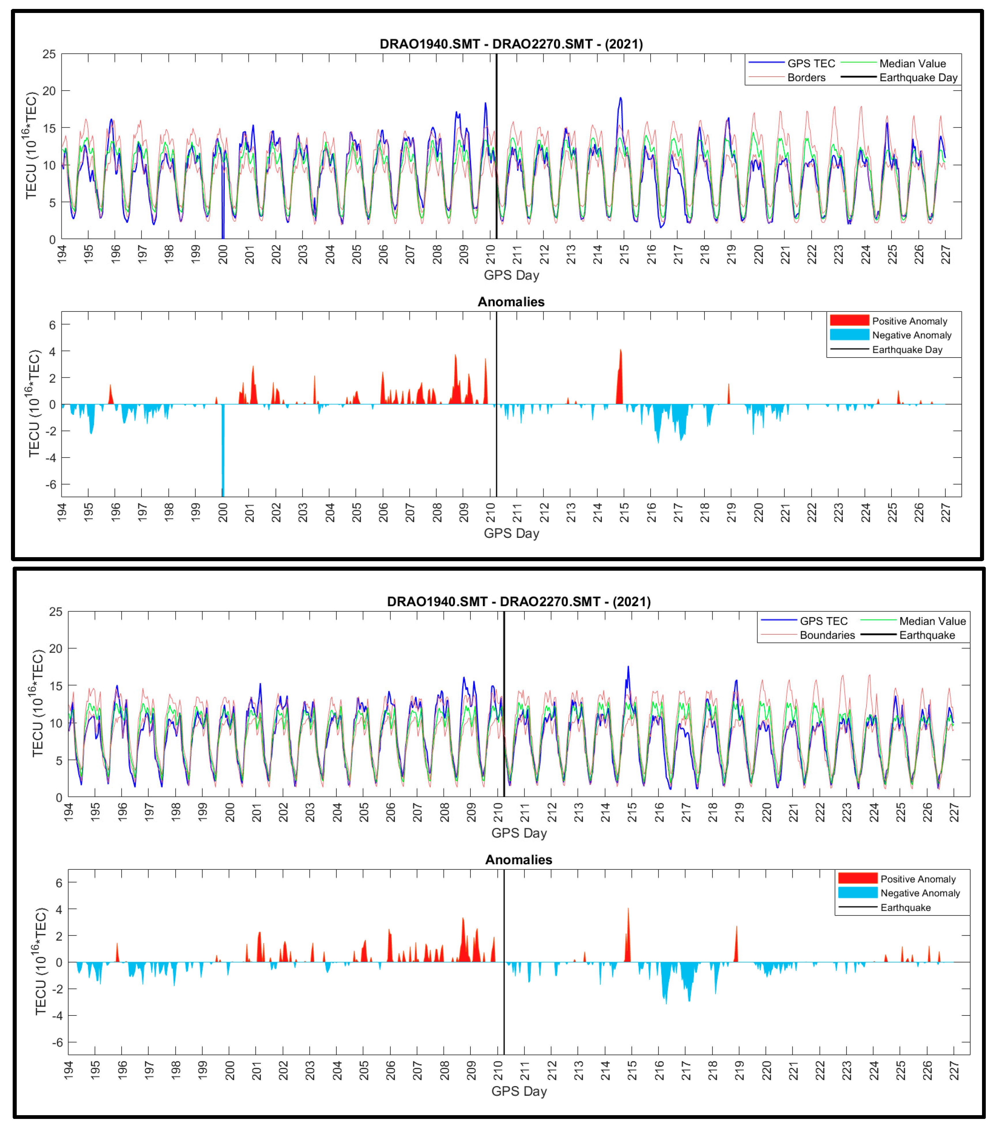
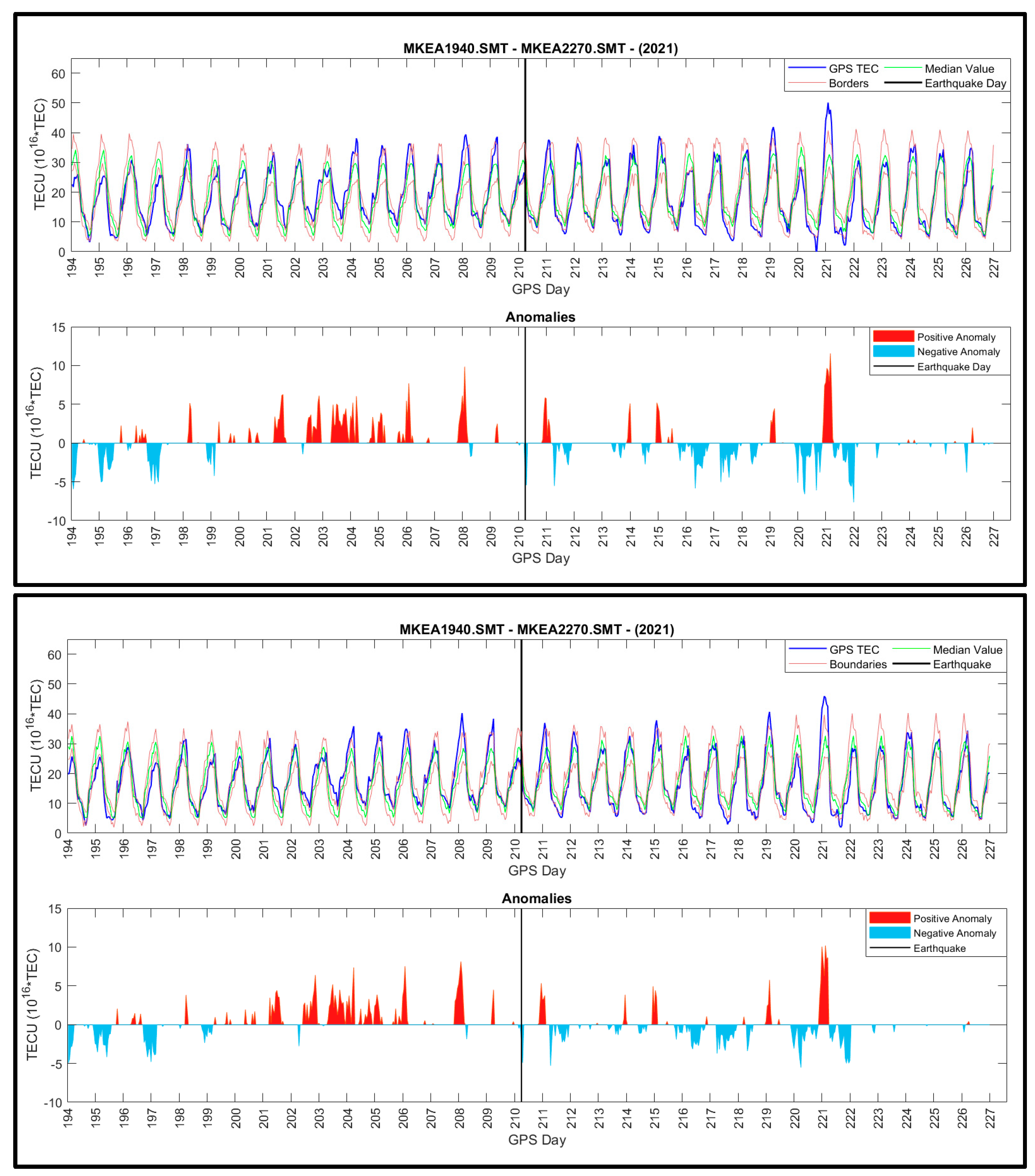
In conclusion, in light of all this information, it has been decided to use the TPS model as a sub-model that is expected to provide more accurate anomaly graphs in the next steps of the VTEC calculations and anomaly studies in this study. Additionally, when comparing the polynomial method with the TPS method based on the obtained results, it is seen that there is an improvement in the std and RMSE values by 1.3% and 5.1% for the WHIT station, 36.5% and 41.3% for the DRAO station, and 21.9% and 43.9% for the MKEA station, respectively. The next step is to calculate the VTEC values for all stations using both the polynomial approach and the TPS method and to obtain the anomaly graphs. Figure 9, Figure 10 and Figure 11 present the anomaly graphs for the stations obtained from polynomial interpolation and the TPS methods.
Space weather conditions, as well as anomaly graphs, should be evaluated together for earthquake precursor analysis. Ref. [13] analyzed the TEC anomalies together with the space weather conditions by conducting precursor research for this earthquake using the polynomial interpolation method. Since the space weather conditions were the same in both studies, the purpose of this study was to investigate the performance of various interpolation methods along with the polynomial method. An examination of Figure 9, Figure 10 and Figure 11 reveals that the graph generated by polynomial integration for the WHIT station has abrupt jumps at the end of the 199th GPS day before the earthquake, and at the end of the 213th GPS day after the earthquake, which do not occur in the graph created using the TPS method. The same situation occurred at the DRAO station at the beginning of the 200th GPS day. The GPS observation data were smoothed to remove outliers and cycle slips during the data preparation process. Therefore, the interpolation method is assumed to be the cause of these current jumps. When the anomalies were analyzed, it was found that similar trends occurred for both positive and negative anomalies in both interpolation methods for all three stations; however, there were some differences of up to 2–2.5 TECU between the two methods for the same anomaly. This case demonstrates the significance of the interpolation method used in the analysis of ionospheric TEC values and earthquake precursor research in order to produce more accurate interpretations.

4. Conclusions

The purpose of this work was to highlight the significance of interpolation techniques for ionospheric studies, especially precursor analysis for earthquakes. In this context, three different IGS stations’ GPS data were used to determine the ionospheric STEC values at ionospheric piercing points. By using the polynomial, kriging point, kriging block, multiquadric, and thin plate spline interpolation techniques, the STEC values of the receiver in the zenith direction were determined. These values were then compared to values obtained from the CODE Analysis Center’s IONEX file. Different accuracy metrics, namely, standard deviation, mean square error, R2, d (Index of Agreement), Pearson’s correlation coefficient, c (confidence index), and Kling–Gupta efficiency (KGE), have been evaluated. According to these metrics, the approach with the highest accuracy was found to be the thin plate spline (TPS) interpolation method. This method complied the VTEC values in the graph where anomalies were formed in the search for earthquake precursors. In this study, anomaly graphs made previously using the polynomial interpolation approach for the same data and earthquake were compared to graphs created using the thin plate spline method. The comparison revealed that the anomaly patterns were similar for both methods, but there were differences in the TEC amounts of up to about 2–2.5 TECU. Furthermore, abrupt jumps in graphs generated with the polynomial interpolation approach were not detected in the graphs created with the thin plate spline method. In this case, the interpolation method has the potential to alter possible anomaly interpretations. This study is presented as an example study in the application of interpolation methods, which aims to determine TEC values more accurately and analyze their changes. For future research, it is suggested that TEC values obtained from different interpolation methods will be taken into consideration for research into the precursors of earthquake and earthquake warning systems, since they determine boundary values and anomaly quantities in anomaly graphs.

Author Contributions

Conceptualization, S.D. and İ.K.; methodology, S.D. and İ.K.; software, S.D. and İ.K.; validation, S.D. and İ.K.; formal analysis, S.D. and İ.K.; investigation, S.D. and İ.K.; resources, İ.K.; data curation, İ.K.; writing—original draft preparation, S.D. and İ.K.; writing—review and editing, S.D. and İ.K.; visualization, S.D. and İ.K.; supervision, S.D.; project administration, S.D.; funding acquisition, S.D. and İ.K. All authors have read and agreed to the published version of the manuscript.

Funding

This research received no external funding.

Institutional Review Board Statement

Not applicable.

Informed Consent Statement

Not applicable.

Data Availability Statement

GPS data for the study were obtained from the NASA/CDDIS (National Aeronautics and Space Administration/Crustal Dynamics Data Information System) website, and data on space climate conditions were obtained from the NASA/GSFC OMNIWEB service website. The authors are grateful to these institutions for sharing their scientific data.

Acknowledgments

This research grew out of a master’s thesis titled “Detection of Ionospheric Anomalies with GNSS and Investigation as an Earthquake Precursor” completed at Konya Technical University’s Department of Geomatics Engineering. We sincerely thank the editorial office and the anonymous reviewers for their insightful comments and constructive suggestions, which have greatly contributed to the improvement of this manuscript.

Conflicts of Interest

The authors declare no conflicts of interest.

References

  1. Wang, C.; Xin, S.; Liu, X.; Shi, C.; Fan, L. Prediction of global ionospheric VTEC maps using an adaptive autoregressive model. Earth Planets Space 2018, 70, 18. [Google Scholar] [CrossRef]
  2. Yildiz, S.K.; Arikan, F. Estimation of planar trend model parameters for midlatitude ionosphere. J. Geophys. Res. Space Phys. 2020, 125, e2019JA027223. [Google Scholar] [CrossRef]
  3. Pikridas, C.; Bitharis, S.; Katsougiannopoulos, S.; Spanakaki, K. Study of TEC variations using permanent stations GNSS data in relation with seismic events. Application on Samothrace earthquake of 24 May 2014. Geod. Cartogr. 2019, 45, 137–146. [Google Scholar] [CrossRef]
  4. Orus, R.; Hernandez-Pajares, M.; Juan, J.M.; Sanz, J. Improvement of global ionospheric VTEC maps by using kriging interpolation technique. J. Atmos. Sol. Terr. Phys. 2005, 67, 1598–1609. [Google Scholar] [CrossRef]
  5. Krypiak-Gregorczyk, A.; Wielgosz, P.; Borkowski, A. Ionospheric model for European region based on multi-GNSS data and TPS interpolation. Remote Sens. 2017, 9, 1221. [Google Scholar] [CrossRef]
  6. Şentürk, E.; Çepni, M.S. Performance of different weighting and surface fitting techniques on station-wise TEC calculation and modified sine weighting supported by the sun effect. J. Spatial Sci. 2019, 64, 209–220. [Google Scholar] [CrossRef]
  7. Ogryzek, M.; Krypiak-Gregorczyk, A.; Wielgosz, P. Optimal geostatistical methods for interpolation of the ionosphere: A case study on the St Patrick’s Day storm of 2015. Sensors 2020, 2, 2840. [Google Scholar] [CrossRef]
  8. Nayak, K.; López-Urías, C.; Romero-Andrade, R.; Sharma, G.; Guzmán-Acevedo, G.M.; Trejo-Soto, M.E. Ionospheric Total Electron Content (TEC) Anomalies as Earthquake Precursors: Unveiling the Geophysical Connection Leading to the 2023 Moroccan 6.8 Mw Earthquake. Geosciences 2023, 13, 319. [Google Scholar] [CrossRef]
  9. Sharma, G.; Nayak, K.; Romero-Andrade, R.; Aslam, M.M.; Sarma, K.K.; Aggarwal, S.P. Low Ionosphere Density Above the Earthquake Epicentre Region of Mw 7.2, El Mayor–Cucapah Earthquake Evident from Dense CORS Data. J. Indian Soc. Remote Sens. 2024, 52, 543–555. [Google Scholar] [CrossRef]
  10. Dong, L.; Zhang, X.; Du, X. Analysis of Ionospheric Perturbations Possibly Related to Yangbi Ms6.4 and Maduo Ms7.4 Earthquakes on 21 May 2021 in China Using GPS TEC and GIM TEC Data. Atmosphere 2022, 13, 1725. [Google Scholar] [CrossRef]
  11. Nayak, K.; Romero-Andrade, R.; Sharma, G.; Zavala, J.L.C.; Urias, C.L. A combined approach using b-value and ionospheric GPS-TEC for large earthquake precursor detection: A case study for the Colima earthquake of 7.7 Mw, Mexico. Acta Geod. Geophys. 2023, 58, 515–538. [Google Scholar] [CrossRef]
  12. Seemala, G.P.; GPS-TEC Analysis Application. Technical Document. 2017. Available online: https://seemala.blogspot.com/ (accessed on 8 August 2024).
  13. Köz, İ.; Doğanalp, S. Investigation of ionospheric anomalies in relation to earthquakes during high and low solar activity periods in years 2002 and 2021. Geomag. Aeron. 2023, 63, 93–104. [Google Scholar] [CrossRef]
  14. Dobrovolsky, I.P.; Zubkov, S.I.; Miachkin, V.I. Estimation of the size of earthquake preparation zones. Pure Appl. Geophys. 1979, 117, 1025–1044. [Google Scholar] [CrossRef]
  15. NASA’s Archive of Space Geodesy Data. Available online: https://cddis.nasa.gov/index.html (accessed on 1 May 2022).
  16. Dach, R.; Lutz, S.; Walser, P.; Fridez, P. (Eds.) Bernese GNSS Software Version 5.2; Astronomical Institute, University of Bern: Bern, Switzerland, 2015; pp. 129–132. [Google Scholar] [CrossRef]
  17. Schaer, S.; Gurtner, W. IONEX: The Ionosphere Map Exchange Format Version 1.1; Astronomical Institute, University of Bern: Bern, Switzerland, 2015; pp. 2–5. [Google Scholar]
  18. Liu, J.Y.; Chen, Y.I.; Chen, C.H.; Liu, C.Y.; Chen, C.Y.; Nishihashi, M.; Li, J.Z.; Xia, Y.Q.; Oyama, K.I.; Hattori, K.; et al. Seismoionospheric GPS total electron content anomalies observed before the 12 May 2008 Mw 7.9 Wenchuan earthquake. J. Geophy. Res. 2009, 114, 1–10. [Google Scholar] [CrossRef]
  19. Khampuengson, T.; Wang, W. Novel Methods for Imputing Missing Values in Water Level Monitoring Data. Water Resour. Manag. 2023, 37, 851–878. [Google Scholar] [CrossRef]
  20. Amoroso, P.P.; Aguilar, F.J.; Parente, C.; Aguilar, M.A. Statistical Assessment of Some Interpolation Methods for Building Grid Format Digital Bathymetric Models. Remote Sens. 2023, 15, 2072. [Google Scholar] [CrossRef]
  21. Surfer Help. Available online: https://surferhelp.goldensoftware.com/griddata/idd_grid_data_kriging.htm (accessed on 21 December 2023).
  22. Huang, L.; Zhang, H.; Xu, P.; Geng, J.; Wang, C.; Liu, J. Kriging with Unknown Variance Components for Regional Ionospheric Reconstruction. Sensors 2017, 17, 468. [Google Scholar] [CrossRef]
  23. Dehvari, A. DEM Application and Qualification with Regard to Terrain Analysis, Land Use Classification and Watershed Modeling. Ph.D. Thesis, The Faculty of Graduate Studies of The University of Guelph, Guelph, Canada, 2010. [Google Scholar]
  24. Arseni, M.; Voiculescu, M.; Georgescu, L.P.; Iticescu, C.; Rosu, A. Testing Different Interpolation Methods Based on Single Beam Echosounder River Surveying. Case Study: Siret River. ISPRS Int. J. Geo-Inf. 2019, 8, 507. [Google Scholar] [CrossRef]
  25. Alsharif, F. Quasi-Interpolation on Chebyshev Grids with Boundary Corrections. Computation 2024, 12, 100. [Google Scholar] [CrossRef]
  26. Sun, J.; Wang, L.; Gong, D. An Adaptive Selection Method for Shape Parameters in MQ-RBF Interpolation for Two-Dimensional Scattered Data and Its Application to Integral Equation Solving. Fractal Fract. 2023, 7, 448. [Google Scholar] [CrossRef]
  27. Özkaya Yılmaz, Ö.; Kayran, A. A Comparative Study on the Efficiencies of Aerodynamic Reduced Order Models of Rigid and Aeroelastic Sweptback Wings. Aerospace 2024, 11, 616. [Google Scholar] [CrossRef]
  28. Foster, M.P.; Evans, A.N. An Evaluation of Interpolation Techniques for Reconstructing Ionospheric TEC Maps. IEEE Trans. Geosci. Remote Sens. 2008, 46, 2153–2164. [Google Scholar] [CrossRef]
  29. Tang, S.; Huang, Z.; Yuan, H. Improving regional ionospheric TEC mapping based on RBF interpolation. Adv. Space Res. 2021, 67, 722–730. [Google Scholar] [CrossRef]
  30. Jasek, K.; Pasternak, M.; Miluski, W.; Bugaj, J.; Grabka, M. Application of Gaussian Radial Basis Functions for Fast Spatial Imaging of Ground Penetration Radar Data Obtained on an Irregular Grid. Electronics 2021, 10, 2965. [Google Scholar] [CrossRef]
  31. Rocha, H. On the selection of the most adequate radial basis function. Appl. Math. Model. 2009, 33, 1573–1583. [Google Scholar] [CrossRef]
  32. Doganalp, S.; Selvi, H.Z. Local geoid determination in strip area projects by using polynomials, least-squares collocation and radial basis functions. Measurement 2015, 73, 429–438. [Google Scholar] [CrossRef]
  33. Carlson, R.E.; Foley, T.A. The parameter R2 in multiquadric interpolation. Computers Math. Applic. 1991, 21, 29–42. [Google Scholar] [CrossRef]
  34. Hardy, R.L. Theory of applications of the multiquadratic–biharmonic method: 20 years of discovery 1968–1988. Comput. Math. Appl. 1990, 19, 163–208. [Google Scholar] [CrossRef]
  35. Rippa, S. An algorithm for selecting a good parameter c in radial basis function interpolation. Adv. Comput. Math. 1999, 11, 193–210. [Google Scholar] [CrossRef]
  36. Fasshauer, G.E. Newton iteration with multiquadrics for the solution of nonlinear PDEs. Comput. Math. Appl. 2002, 43, 423–438. [Google Scholar] [CrossRef]
  37. Bildirici, I.O. Numerical inverse transformation for map projections. Comput. Geosci. 2003, 29, 1003–1011. [Google Scholar] [CrossRef]
  38. Ferdowsi, M.; Gan, M.-H.; Kwan, B.-H.; Tan, M.P.; Goh, C.-H. Anticipating Fainting: Real-Time Prediction of Vasovagal Syncope During Head-Up Tilt Table Testing. In Proceedings of the TENCON 2023—2023 IEEE Region 10 Conference (TENCON), Chiang Mai, Thailand, 31 October–3 November 2023; pp. 1–6. [Google Scholar] [CrossRef]
  39. Gizachew, S.; Sitotaw, B.; Mengistu, G. Annual Mean and Correlation of Global Vertical Total Electron Content from Various Global Data Centers. Am. J. Astron. Astrophysic. 2020, 8, 1–7. [Google Scholar] [CrossRef]
  40. Willmott, C.J. On the Validation of Models. Phys. Geogr. 1981, 2, 184–194. [Google Scholar] [CrossRef]
  41. Onyutha, C. A hydrological model skill score and revised R-squared. Hydrol. Res. 2022, 53, 51–64. [Google Scholar] [CrossRef]
  42. Ruezzene, C.B.; Miranda, R.B.; Bolleli, T.M.; Mauad, F.F. Filling and validating rainfall data based on statistical techniques and artificial intelligence. Rev. Ambient. Água 2021, 16, e2767. [Google Scholar] [CrossRef]
  43. Hafizi, H.; Sorman, A.A. Integrating Meteorological Forcing from Ground Observations and MSWX Dataset for Streamflow Prediction under Multiple Parameterization Scenarios. Water 2022, 14, 2721. [Google Scholar] [CrossRef]
  44. Pham, L.T.; Luo, L.; Finley, A. Evaluation of random forests for short-term daily streamflow forecasting in rainfall-and snowmelt-driven watersheds. Hydrol. Earth. Syst. Sc. 2021, 25, 2997–3015. [Google Scholar] [CrossRef]
Figure 1. Study area.
Atmosphere 15 00986 g001
Figure 2. Demonstration of IPPs [13].
Atmosphere 15 00986 g002
Figure 3. Comparison between CODE IONEX file with polynomial, KrigingP, KrigingB, MQ, TPS for WHIT station.
Atmosphere 15 00986 g003
Figure 4. Comparison between CODE IONEX file with polynomial, KrigingP, KrigingB, MQ, TPS for DRAO station.
Atmosphere 15 00986 g004
Figure 5. Comparison between CODE IONEX file with polynomial, KrigingP, KrigingB, MQ, TPS for MKEA station.
Atmosphere 15 00986 g005
Figure 6. The differences between TEC values of interpolation methods and CODEIONEX reference data for WHIT station.
Atmosphere 15 00986 g006
Figure 7. The differences between TEC values of interpolation methods and CODEIONEX reference data for DRAO station.
Atmosphere 15 00986 g007
Figure 8. The differences between TEC values of interpolation methods and CODEIONEX reference data for MKEA station.
Atmosphere 15 00986 g008
Figure 9. Anomaly graphs of WHIT stations using polynomial interpolation (top) and thin plate spline interpolation (bottom) methods.
Atmosphere 15 00986 g009
Figure 10. Anomaly graphs of DRAO stations using polynomial interpolation (top) and thin plate spline interpolation (bottom) methods.
Atmosphere 15 00986 g010
Figure 11. Anomaly graphs of MKEA stations using polynomial interpolation (top) and thin plate spline interpolation (bottom) methods.
Atmosphere 15 00986 g011
Table 1. Evaluation metrics for all stations. The numbers in bold represent the best accuracies of the relevant station criteria.
StationCriteriaCODE-PolyCODE-KrigingPCODE-KrigingBCODE-MQCODE-TPS
WHITmin−16.100−3.679−4.569−4.355−5.495
mean−0.389−0.664−1.211−0.0830.162
max16.9003.5982.8865.8257.148
std1.2370.9590.9451.1171.221
RMSE1.2971.1661.5361.1201.231
R20.8520.9170.9320.8670.833
IA0.9490.9590.9330.9600.950
Pearson0.9230.9580.9660.9310.913
c0.8760.9180.9010.8940.867
KGE0.8170.8250.7790.8560.856
StationCriteriaCODE-PolyCODE-KrigingPCODE-KrigingBCODE-MQCODE-TPS
DRAOmin−3.600−3.369−3.941−3.558−3.743
mean−0.495−0.433−0.972−0.0560.044
max33.5001.9051.5382.0612.090
std1.1970.7560.7890.7540.760
RMSE1.2950.8711.2520.7560.760
R20.9160.9660.9720.9600.958
IA0.9700.9860.9730.9890.989
Pearson0.9570.9830.9860.9800.979
c0.9290.9690.9600.9690.968
KGE0.8690.9070.8440.9510.961
StationCriteriaCODE-PolyCODE-KrigingPCODE-KrigingBCODE-MQCODE-TPS
MKEAmin−7.700−7.776−9.177−6.347−6.125
mean−1.909−1.701−2.445−0.932−0.738
max4.8002.0420.6262.6642.668
std1.4271.4011.5491.2111.114
RMSE2.3842.2042.8941.5271.336
R20.9830.9820.9850.9830.985
IA0.9830.9850.9760.9930.994
Pearson0.9920.9910.9920.9910.992
c0.9750.9760.9680.9840.987
KGE0.8670.8820.8320.9370.951
Disclaimer/Publisher’s Note: The statements, opinions and data contained in all publications are solely those of the individual author(s) and contributor(s) and not of MDPI and/or the editor(s). MDPI and/or the editor(s) disclaim responsibility for any injury to people or property resulting from any ideas, methods, instructions or products referred to in the content.