Article

Air Quality Prediction and Ranking Assessment Based on Bootstrap-XGBoost Algorithm and Ordinal Classification Models

1
School of Mathematics and Statistics, Northwest Normal University, Lanzhou 730070, China
2
Big Data Intelligence Centre, The Hang Seng University of Hong Kong, Hong Kong, China
*
Authors to whom correspondence should be addressed.
Atmosphere 2024, 15(8), 925; https://doi.org/10.3390/atmos15080925
Submission received: 23 June 2024 / Revised: 16 July 2024 / Accepted: 26 July 2024 / Published: 2 August 2024
(This article belongs to the Special Issue Atmospheric Pollutants: Monitoring and Observation)

Abstract

:
Along with the rapid development of industries and the acceleration of urbanisation, the problem of air pollution is becoming more serious. Exploring the relevant factors affecting air quality and accurately predicting the air quality index are significant in improving the overall environmental quality and realising green economic development. Machine learning algorithms and statistical models have been widely used in air quality prediction and ranking assessment. In this paper, based on daily air quality data for the city of Xi’an, China, from 1 October 2022 to 30 September 2023, we construct support vector regression (SVR), gradient boosting decision tree (GBDT), extreme gradient boosting (XGBoost), random forests (RF), neural network (NN) and long short-term memory (LSTM) models to analyse the influence of the air quality index for Xi’an and to conduct comparative tests. The predicted values and 95% prediction intervals of the AQI for the next 15 days for Xi’an, China, are given based on the Bootstrap-XGBoost algorithm. Further, the ordinal logit regression and ordinal probit regression models are constructed to evaluate and accurately predict the AQI ranks of the data from 1 October 2023 to 15 October 2023 for Xi’an. Finally, this paper proposes some suggestions and policy measures based on the findings of this paper.

1. Introduction

As industrialisation and urbanisation advance and urban energy consumption increases, the world faces a certain degree of regional and compounded air pollution problems. The deterioration of the ecological environment caused by atmospheric environmental problems has become increasingly evident and is closely related to human health, which has become a significant public health problem. Relevant studies [1,2,3] have shown that severe air pollution can cause a variety of respiratory diseases, such as chronic pharyngitis, chronic bronchitis, and bronchial asthma, and there is a significant correlation between exposure to atmospheric particulate matter and near-surface ozone and the number of morbidities and deaths due to chronic cardiovascular diseases. In addition, severe air pollution exacerbates haze conditions and reduces visibility in the near-air layer, leading to several problems, such as traffic congestion and flight delays [4]. This issue is consistent with the Sustainable Development Goals (SDGs) of “good health and well-being” and “sustainable cities and communities”, which emphasise the importance of addressing environmental health risks and promoting sustainable urban development. Therefore, it is of great significance to explore the influence of changes in air pollutant concentrations and various factors and to establish an urban air quality prediction model with high efficiency and accuracy to promote the prevention and control of air pollution in the country.
Currently, methods for analysing and predicting quality are divided into two main categories: statistical methods and machine learning algorithms. Statistical methods are mostly linear studies, which mainly use traditional modelling strategies to predict air quality [5]. For example, Niu et al. [6] used the auto-regressive moving average model to study the composite air quality index for Chengdu. The results of the study showed that the air quality in Chengdu had no improving trend in the coming period. Jian et al. [7] predicted airborne particulate matter concentrations via the auto-regressive integrated moving average model. Abedi et al. [8] used the auto-regressive distributed lag (ARDL) model to study the relationship between air pollution and respiratory and cardiovascular diseases. The results showed that for every 10-unit increase in the AQI, the number of hospitalisations for cardiovascular diseases increased by 7.3%. Woldu [9] used the ARDL model to study the bidirectional causal relationship between urban globalisation and CO2 emissions in Mozambique. With its rapid development, new-generation information technology such as big data analytics and machine learning can perform analysis and prediction by learning data patterns and optimising algorithms [10,11,12,13]. Because of its high accuracy and reliability, many scholars use different machine learning algorithms to study and predict air quality. Biancofiore et al. [14] used a recursive neural network model that allows one to obtain real-time information on PM10 and PM2.5 in Adriatic coastal cities. Yang et al. [15] used a space–time support vector regression model to predict hourly PM2.5 concentrations. Pawul [16], based on Polish National Environmental Monitoring System data and meteorological data, developed a neural network model for air pollutant prediction. Ma et al. [17] performed an impact analysis of air quality based on an extreme gradient boosting model. The results of the study showed that six factors, such as personal income and power plant density, have the greatest impact on air quality in the United States. Zhao et al. [18] integrated forward neural networks and recurrent neural networks to predict air quality hourly in northwestern China. Bekkar et al. [19] performed the hour-by-hour forecasting of PM2.5 concentration in Beijing based on a neural network with a long short-term memory network model. Huang et al. [20] used spatio-temporal information to forecast air quality through deep convolutional networks. Samad et al. [21] used five machine learning models, such as ridge regression, support vector regression, and random forest, to study pollutant concentrations at monitoring sites. Zhang et al. [22] used a spatial transform network model to forecast PM2.5 concentrations in the next 6, 12, 24, and 48 h in Beijing and Taizhou. In addition, many other scholars have studied and forecasted the air quality ranks. Liu et al. [23] forecasted the air quality ranks for Bayannur based on an integrated model of stepwise regression, principal component analysis, and BP neural network (STEPDISC-PCA-BP). Ratković et al. [24] accurately predicted air quality levels in the next hour in a city in Montenegro by using a hybrid LSTM model. Zhao et al. [25] proposed a detailed examination model of air quality with a co-training semi-supervised learning approach.
This paper proposes to model and predict the daily air quality data from 1 October 2022 to 30 September 2023 in the city of Xi’an, China, by using the Bootstrap-XGBoost algorithm and ordinal classification models. This paper is organised as follows: Section 2 preprocesses the data and draws the stacked plot of air quality percentage to study the seasonality of air pollution in Xi’an, China, in recent years; Section 3 constructs the SVR model, the GBDT model, the XGBoost model, the RF model, the NN model, and the LSTM model to compare the predictions on the test set, and the Bootstrap-XGBoost algorithm is proposed based on the best-performing XGBoost model combined with the Bootstrap method, based on which the predicted values and prediction intervals of the AQI for the next 15 days in Xi’an, China, are given; Section 4 forecasts the AQI ranks for the next 15 days based on the ordinal logit and ordinal probit regression models; Section 5 proposes the targeted recommendations and improvement measures based on the results of the study. The research framework of this paper is shown in Figure 1.

2. Data Sources and Preprocessing

This section gives a clear explanation of the data sources used in this study and their descriptive analysis.

2.1. Data Sources

The data in this paper come from the data published on the official statistics website of China Air Quality Online Testing Platform (https://www.aqistudy.cn/historydata/ (accessed on 29 November 2023)), and daily air quality data for one year from 1 October 2022 to 30 September 2023 were collected for Xi’an, China.
The data used in this paper include the air quality index (AQI) and the concentrations of six pollutants: sulphur dioxide (SO2), nitrogen dioxide (NO2), fine particulate matter (PM2.5), carbon monoxide (CO), particulate matter (PM10), and ozone (O3). The basic information about these data and the related descriptions are shown in Table 1. In 1999, the United States Environmental Protection Agency (USEPA) established the AQI as a quantitative way of interpreting air quality [26]. The individual indexes of the six criteria pollutants are calculated by Equation (1), and the maximum value is determined as the AQI. The higher the AQI, the more severe the air pollution and the greater the risk to human health.
I p = I H i I L o B P H i B P L o C p B P L o + I L o .
where I p is the index for pollutant p, C p is the truncated concentration of pollutant p, B P H i is the concentration breakpoint that is greater than or equal to C p , B P L o is the concentration breakpoint that is less than or equal to C p , I H i is the AQI value corresponding to B P H i , and I L o is the AQI value corresponding to B P L o .

2.2. Data Preprocessing and Seasonal Air Pollution Percentage Analysis

Data preprocessing is the first step to establishing a statistical learning model, and this paper uses the interpolation method and imputed package in R to fill in the missing values; the interpolation method formula is
X ^ = 2 X t X t 1 .
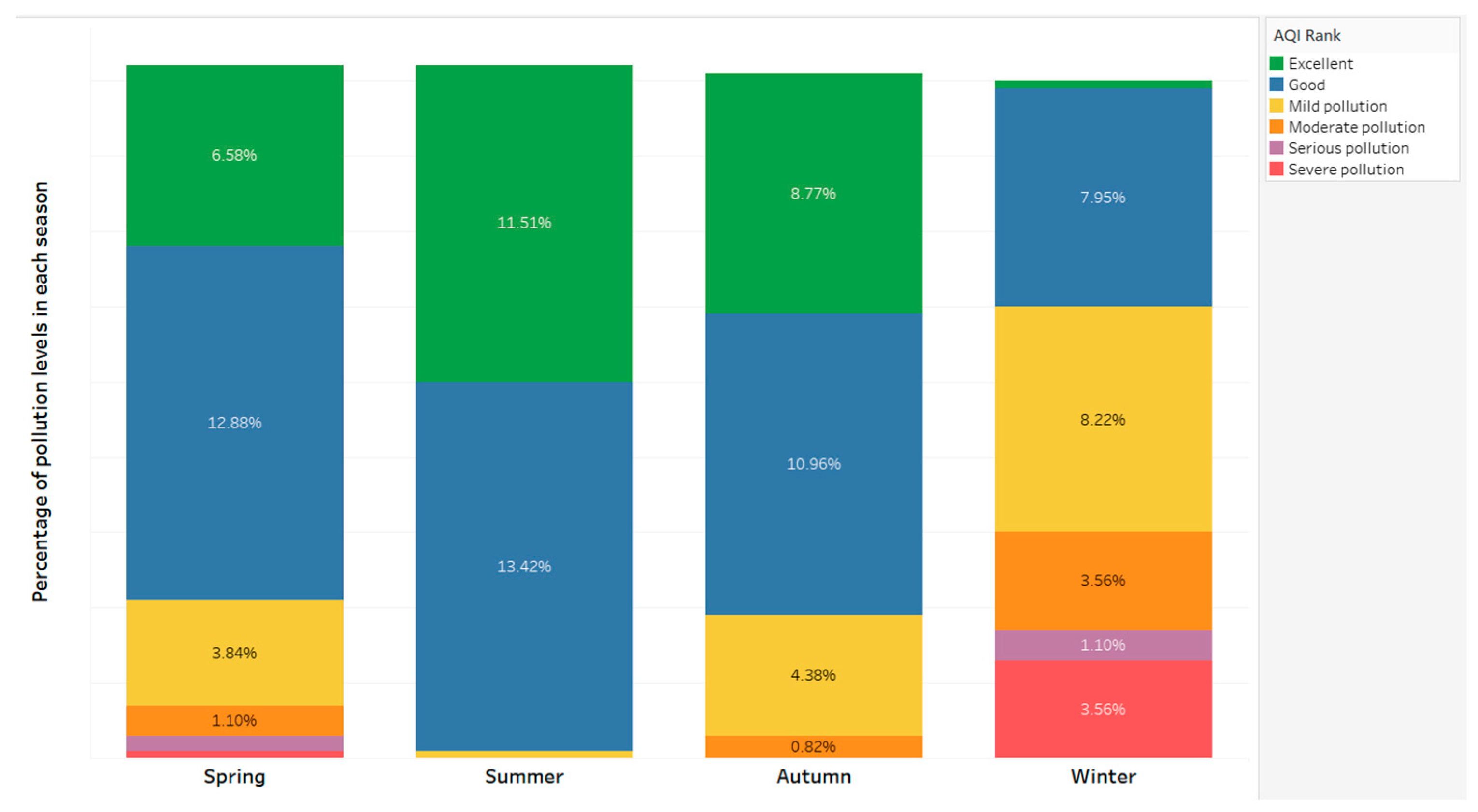
It is stipulated that December to February is winter, March to May is spring, June to August is summer, and September to November is fall. With the help of Tableau software 2024.2.0 (20242.24.0613.1930), the day-by-day air quality pollution levels in Xi’an, China, were counted, and the proportions of each of the six pollutant levels were calculated in each of the four seasons and analysed seasonally, as shown in Figure 2.
It is obvious from Figure 2 that the air quality in Xi’an, China, in the past year was mainly “Good”, accounting for 45.21% of the total data. In summer, the degree of air pollution was the smallest, and the air quality was the best, mainly “Good” and “Excellent”; the air quality in spring and fall was “Excellent” and “Good”, second only to summer, with an increase in the number of “Mild pollution” days and some days being also accompanied by “Moderate pollution” and average air quality; with the arrival of cold air, the number of days with air quality of “Mild pollution” and above in Xi’an, China, in winter accounted for 16.44%, which is more than twice the number of days with air quality of “Excellent” and “Good”. Especially in winter, Xi’an is characterised by severe haze and poor air quality. This is due to the city’s geographical location and climate conditions. During the winter months, Xi’an experiences temperature inversions, which trap pollutants close to the ground, leading to a buildup of particulate matter and other air pollutants. Additionally, the increased heating demand in winter leads to greater emissions from coal-fired power plants and residential heating sources, further exacerbating the air quality issues. As a result, the air situation in Xi’an is not optimistic during the autumn and winter seasons.

3. Empirical Analysis of AQI Prediction

In this section, the selected dataset are empirically analysed by using SVR, GBDT, XGBoost, RF, NN, and LSTM models. In this case, 80% of the dataset is the training set, and 20% is the test set.

3.1. Analysis Based on SVR Model

SVR is a machine learning algorithm for classification and regression that utilises a kernel function to map the data into a high-dimensional space [27]. It searches for the optimal hyperplane to separate different categories of data, thus realising classification or regression prediction.
Let a set of training data be ( x i , y i ) , where x i R d is the feature vector of the ith sample and y i R d is the true value of the ith sample. The objective function of the SVR model can be expressed as
m i n w , b 1 2 w 2 + C i = 1 n [ y i f ( x i ) ] 2 .
where w is the weight vector, b is the bias term, C is the regularisation parameter, and w 2 is the L 2 norm of the weight vector.

3.2. Analysis Based on GBDT Model

GBDT is an integrated machine learning algorithm based on the Boosting strategy proposed by Friedman (2001) [28]. It is an iterative decision tree algorithm consisting of multiple decision trees. The results obtained from each decision tree are accumulated to become the final result, and it is also one of the methods with the best performance in statistical learning. The specific implementation process of the GBDT classifier is as follows.
  • Initialise the learner:
f 0 ( x ) = argmin i = 1 N L ( y i , C ) ,
2.
For each tree m = 1,2 , , M and each sample i = 1,2 , , N , calculate the corresponding negative gradient, i.e., residuals
r i m = L ( y i , f ( x i ) ) f ( x i ) .
where f x i   is the predicted value of the weak learner and y i is the true value of the weak learner.

3.3. Analysis Based on XGBoost Model

XGBoost is a supervised learning model based on combining classifiers with lower classification accuracy into a classifier model with higher accuracy, mainly to reduce the model error [29]. It is a model that is based on the combination of multiple CART trees and has a strong generalisation ability. The algorithm uses the tree as a base classifier, expands the loss function to the second-order derivative by Taylor’s formula, and adds a regular term to the objective loss function, thus avoiding an overly complex model. The objective function is
P x = L x + E x ,
where L x is the loss function, which measures how well the model fits on the training dataset, and E x is the canonical term, which measures the complexity of the model. If the model generates j trees and the base learner model is
y i = j = 1 J f j x i , f j F ,
where f j is one of the base classifiers in F , J is the number of base classifiers, and F is the set of all base classifiers, then the objective function of the XGBoost model is
P x = i = 1 n L y i , y ^ i + j = 1 J E f j .

3.4. Analysis Based on RF Model

RF is an integrated learning method proposed by Breiman [30] which is commonly used for classification, regression, and other machine learning tasks. The principle is to construct a large number of decision trees during training, each of which is unrelated to the others; when a new sample enters the algorithm, each decision tree makes a judgment separately, and each identifies which category the sample should belong to. Further, according to the votes on the classification tree, the sample is classified into a category. The flow of the algorithm is shown in Figure 3. RF is a robust integration algorithm based on a bagging decision tree that realises RF’s random split selection, effectively correcting the problem of decision tree fitting.

3.5. Analysis Based on NN Model

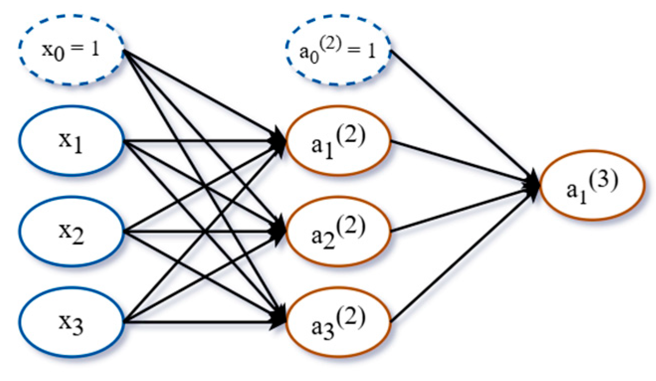
NN is a computational model inspired by the human nervous system. It consists of many interconnected neurons that transmit and process information through weights. A neural network usually consists of multiple layers, including input, hidden, and output layers. It is often used to solve complex pattern recognition and machine learning problems. The input layer receives raw data, the hidden layer processes and extracts features from the input data, and the output layer generates the final output. The connection weight of each neuron in the network determines how much the input affects the output. In Figure 4, x i i = 1,2 , 3   is the value of the input layer, and a i ( k ) ( k = 1,2 , , K ; i = 1,2 , , N k )   denotes the activation value of the ith neuron (the output of that neuron) in the kth layer.

3.6. Analysis Based on LSTM Model

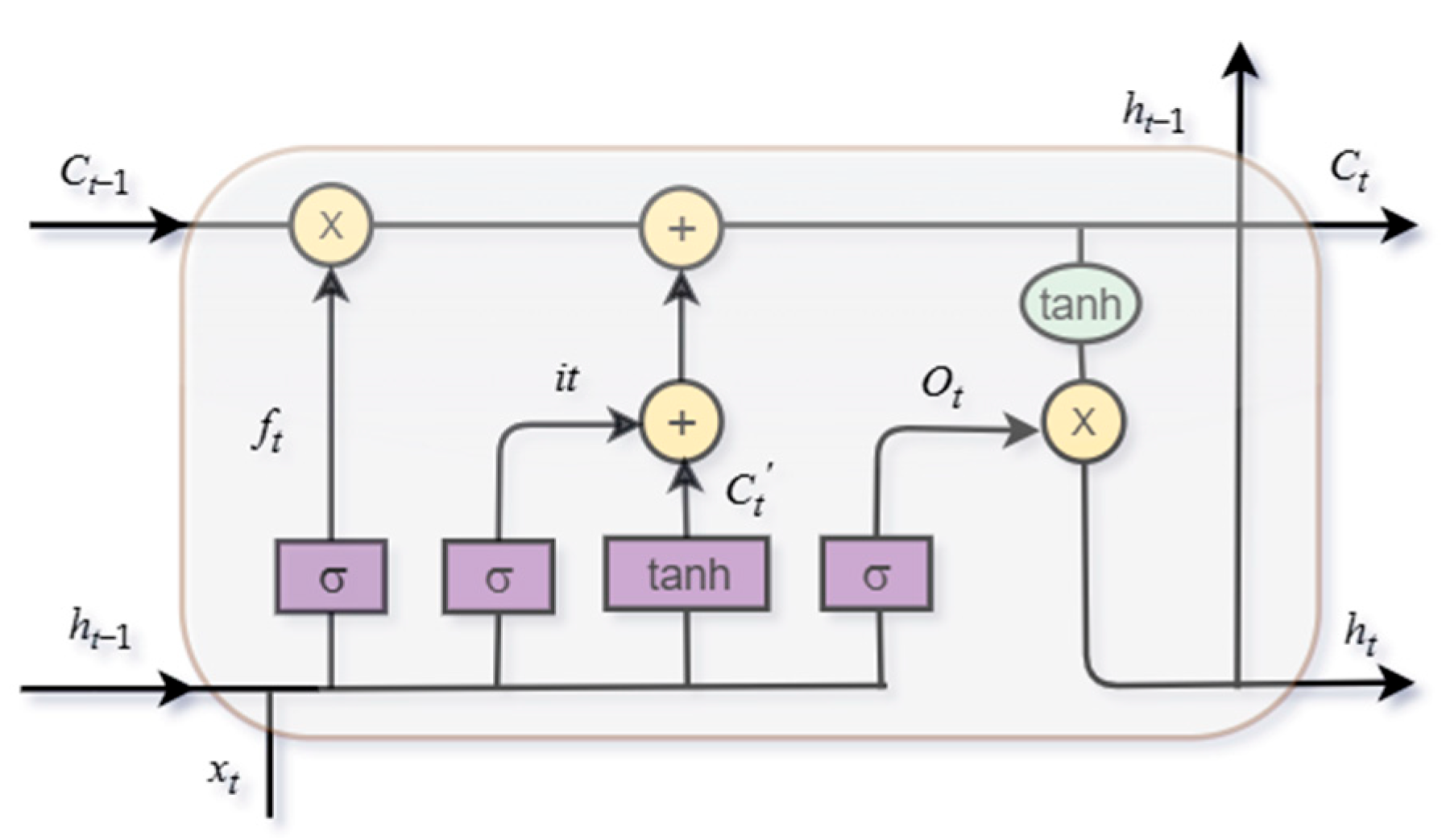
Hochreiter and Schmidhuber proposed the LSTM model in the late 1990s [31]; it is a variant of the traditional RNN. Compared with the traditional neural network model, LSTM can deal with the long-term dependence problem of temporal data and, at the same time, avoid the gradient vanishing problem. It can effectively capture long-term dependencies in sequence data by introducing mechanisms such as memory units, input gates, forgetting gates, and output gates combined with the error back-propagation algorithm. The structural flowchart of the LSTM model is shown in Figure 5.

3.7. Forecast Results and Comparative Analysis

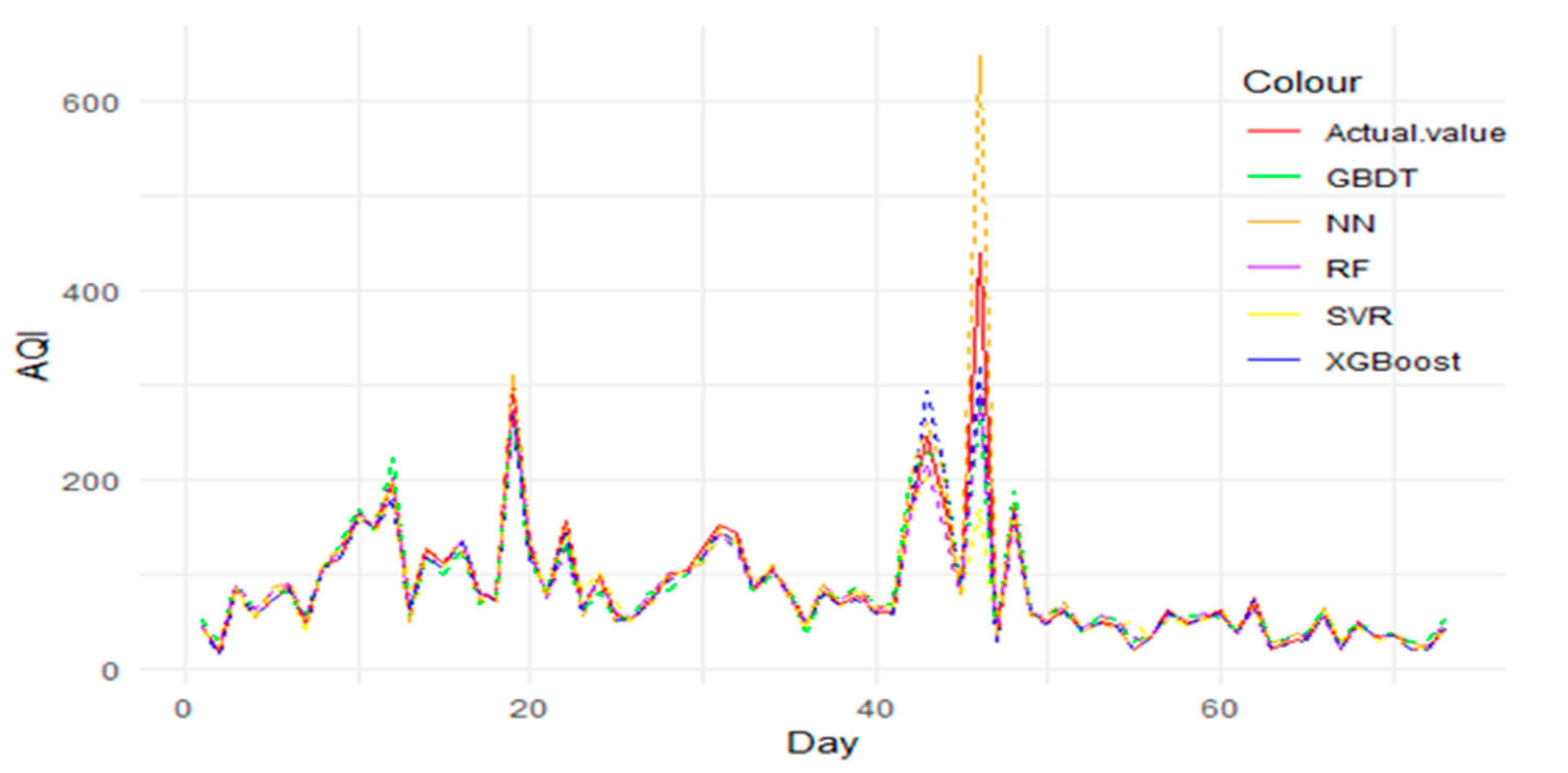
By preprocessing the data, the AQI values were predicted by using the above models in the test set, and the actual and predicted values are shown in Figure 6. It can be seen that the five models have similar prediction trends for the AQI and that the predicted values are close to the true values, indicating that the models can capture the relationships between the AQI and the concentrations of the six pollutants better and that the models are well characterised.

3.8. Model Evaluation

In order to assess the effectiveness of different models in fitting the AQI, four evaluation indexes, namely, Mean Absolute Error (MAE), Root Mean Square Error (RMSE), Mean Absolute Percentage Error (MAPE), and Goodness-of-Fit (R-squared) were selected to evaluate the results of the six model fits in this paper.
M A E ( y , y ^ ) = 1 n i = 1 n y i y ^ i , R M S E ( y , y ^ ) = 1 n i = 1 n ( y i y ^ i ) 2 , M A P E y , y ^ = 100 % n i = 1 n y i y ^ i y i , R 2 = 1 S S E S S T = 1 i = 1 n ( y i y ^ i ) 2 i = 1 n ( y i y ¯ ) 2 .
where y i is the AQI observation of the ith sample, y ^ i is the AQI prediction of the ith sample, and y ¯ is the sample mean. Smaller MAE, RMSE, and MAPE and larger R-squared mean better final prediction. The fitting results are shown in Table 2. From the table, one can see that the MAE and the MAPE values of fitting using the XGBoost model are the smallest and that the R-squared value is the largest. Therefore, the XGBoost model was used to predict the AQI for Xi’an, China, with the smallest error and the best fit, so the following is based on the model to predict the AQI for the next 15 days.

4. AQI Prediction Based on Bootstrap-XGBoost

The bootstrap method is a resampling method in statistics that is used to give the standard error of prediction and prediction interval in predictive analysis. In this paper, time-series data were considered, so the residual Bootstrap method was used, and the prediction in each cycle of the Bootstrap method adopted the XGBoost model. The specific algorithm flow is shown in Algorithm 1.
Algorithm 1: The Bootstrap-XGBoost algorithm
1 :   Input :   Dataset   x t , y t ; B : Bootstrap sample size
2 :   Output :   The   B times Boostrap prediction results
3 :   Fitting   a   model   to   the   preprocessed   data :   y t = f ( x t ) + ε t
4 :   Prediction   of   preprocessed   data :   y ^ t = f ^ ( x t )
5 :   Calculation   of   prediction   residuals :   ε t = y t y ^ t
6: Residual Bootstrap step:
7 :   Setting   the   number   of   resampling   times   B
8 :   f o r   b = 1,2 , , B
9 :   { A   new   sample   ε t b   is   obtained   by   resampling   ε t
10 :     ε t ( b ) s a m p l e ( ε t , r e p l a c e = T R U E )
11 :     Getting   new   samples :   y t ( b ) = y ^ t + ε t ( b )
12 :     The   Bootstrap   prediction   result   y ^ t ( b )   is   obtained   by   fitting   the   new   sample   via   the   XGBoost   algorithm :   ( x t , y t ( b ) ) y ^ t ( b ) = f ^ b ( x t )   }
13 :   Based   on   a   series   of   y ^ t ( b ) , the prediction standard deviation and 95% prediction interval are calculated
Based on the proposed Bootstrap-XGBoost algorithm, the standard deviation and 95% prediction intervals of the predicted AQI for the next 15 days in Xi’an, China, were obtained by setting B = 500 times, as shown in Table 3.
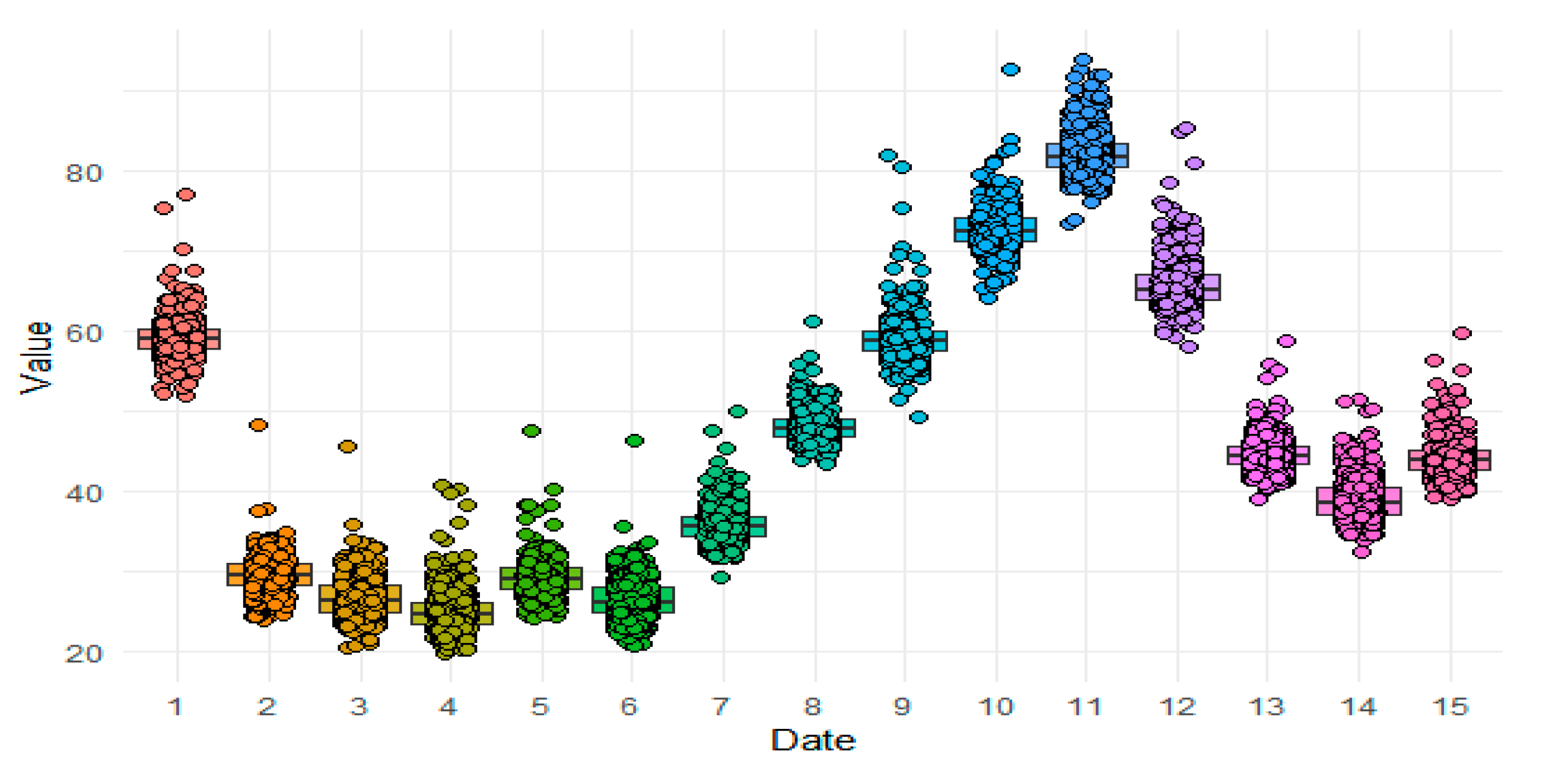
Table 3 and Figure 7 show that the actual values generally fall within the 95% prediction interval of the prediction. The accuracy of the prediction for more days in the future is high, which indicates that the prediction of the future short-term AQI using the Bootstrap-XGBoost method has a high degree of reliability and accuracy and that the prediction for long periods needs to take into account other influencing factors.

5. AQI Rank Assessment

The ordinal logit and probit models are generalised linear models used to establish the relationship between ordinal categorical variables and independent variables and are commonly used in biomedicine, socioeconomics, and machine learning.

5.1. Ordinal Logit Model and Ordinal Probit Model

In this section, the response variable AQI ranks are classified into six categories, namely, “Excellent”, “Good”, “Mild pollution”, “Moderate pollution”, “Severe pollution”, and “Serious pollution”, and based on the following two models, the AQI ranks for Xi’an, China, are evaluated and further predicted from 1 October 2023 to 15 October 2023, in terms of AQI ranks.
Assuming that the response y i { 1,2 , , C } are the ordinal variables and the predictor variables are X = ( x 1 , x 2 , , x k ) T , the expression of the ordinal logit regression model is
L o g i t [ P ( y i j ) ] = log P ( y i j ) P ( y i > j ) = α j + x i T β , i = 1,2 , , n ; j = 1,2 , , C ,
The ordinal probit regression model expression is
Φ 1 [ P ( y i j ) ] = α j + x i T β , i = 1,2 , , n ; j = 1,2 , , C .
where x i = ( x i 1 , x i 2 , , x i k ) T   denotes the k pollutant concentration indicators affecting the AQI, β is the regression coefficient, α 1 α j is the model intercept, and Φ ( ) is the cumulative distribution function of the standard normal distribution.

5.2. Model Estimation Results

The results of parameter estimation using the above two models are shown in Table 4. Based on a p-value of less than 0.05, it can be concluded that PM2.5, PM10, SO2, and O3 concentrations have the most significant effect on the AQI rank, which means that the higher the concentration of this pollutant, the more serious the air pollution situation is, and the higher the AQI rank is (Table 4).
According to Equation (10) and Table 4, the probability of each category of the AQI rank for Xi’an, China, under the ordinal logit regression model can be obtained by
P 1 = exp ( 9.5826 + E s t i m a t e L ) 1 + exp ( 9.5826 + E s t i m a t e L ) P 2 = exp ( 23.2516 + E s t i m a t e L ) 1 + exp ( 23.2516 + E s t i m a t e L ) P 1 P 3 = exp ( 34.9270 + E s t i m a t e L ) 1 + exp ( 34.9270 + E s t i m a t e L ) P 1 P 2 P 4 = exp ( 46.4949 + E s t i m a t e L ) 1 + exp ( 46.4949 + E s t i m a t e L ) P 1 P 2 P 3 P 5 = exp ( 67.1061 + E s t i m a t e L ) 1 + exp ( 67.1061 + E s t i m a t e L ) P 1 P 2 P 3 P 4
where E s t i m a t e L = 0.1729 P M 2.5 + 0.1033 P M 10 0.3825 S O 2 + 0.0415 N O 2 + 0.0379 O 3 1.2952 C O , P 1 , P 2 , P 3 , P 4 and P 5 represent the probability of having an the AQI ranks of “Excellent”, “Good”, “Mild pollution”, “Moderate pollution”, “Severe pollution”, and “Serious pollution”, respectively.
According to Equation (11) and Table 4, the probability of each category of AQI rank for Xi’an, China, under the ordinal probit regression model can be obtained by
P 1 = Φ ( 5.4850 + E s t i m a t e P ) P 2 = Φ ( 14.0113 + E s t i m a t e P ) P 1 P 3 = Φ ( 20.7566 + E s t i m a t e P ) P 1 P 2 P 4 = Φ ( 28.0236 + E s t i m a t e P ) P 1 P 2 P 3 P 5 = Φ ( 41.2004 + E s t i m a t e P ) P 1 P 2 P 3 P 4
where E s t i m a t e P = 0.1109 P M 2.5 + 0.0632 P M 10 0.2405 S O 2 + 0.0170 N O 2 + 0.0224 O 3 0.9499 C O .

5.3. AQI Ranking Forecast

The accuracy of predicting AQI rankings on the test set based on the ordinal logit regression and ordinal probit regression models developed in Section 5.1 and Section 5.2 is shown in Table 5. As can be seen from Table 5, the prediction accuracy of both the ordinal logit regression and ordinal probit regression models is above 86%, which is high, and the AQI ranks for Xi’an, China, for the period from 1 October to 15 October 2023, were predicted using these two models.
Table 6 shows that the predictions for the next 15 days based on the two models are entirely consistent with the actual results, and the prediction probabilities are mostly high, indicating that the two models have a good prediction effect on the AQI ranks.

6. Conclusions and Suggestions

In this paper, the prediction of AQI by PM2.5, PM10, SO2, NO2, O3, and CO is investigated by building SVR, GBDT, XGBoost, RF, NN, and LSTM models and comparing the prediction results on the test set. It is found that the XGBoost model has the best prediction effect. Thereby, we propose a robust Bootstrap-XGBoost algorithm to give the AQI prediction values and 95% prediction intervals for the next 15 days in Xi’an, China, and the results show that most of the predicted values coincide with the true values and that the prediction intervals are covered by more than 70%. In addition, in this paper, we fit the air quality classes based on ordinal logit and ordinal probit regression models and forecast the AQI classes from 1 October to 15 October 2023, in Xi’an, China. The results show that the prediction accuracy of both ordinal models is 100%.
Based on the above conclusions, this paper proposes some applicable recommendations and targeted initiatives to improve air quality in Xi’an.
(1) As one of the megacities in China, preventing and controlling particulate pollution in Xi’an has been crucial in recent years. Based on continuing to maintain emission reduction, the prevention and control of gaseous pollutants (especially O3 and SO2) should be strengthened. The main goals for the present and future are the synergistic prevention and control of atmospheric particulate matter and O3 and introducing related policy and standards on VOC management—for example, centralised heating, optimised motor vehicle travel restrictions, and increased vegetation cover. In addition, it is also necessary to raise public awareness of air pollution prevention and control.
(2) The air in Xi’an is dry, and in spring and winter, the soil has low water content, which can easily bring dust into the air in windy weather. Relevant governments should strengthen the monitoring of dust from construction sites and material stacking sites in urban areas and urge construction units to cover the bare-ground surface in a timely manner. At the same time, regular urban sanitation sweeps should be carried out to pick up garbage, wipe down fences, clean up roads, and spray on time to ensure the city is clean and tidy.
(3) As one of the cities with a modern industrial system developed, it is essential to maintain the synergistic development of the green economy and create a better living environment by improving the resource utilisation rate in Xi’an, optimising the energy structure and industrial layout, continuing to carry out the comprehensive treatment of multi-pollution sources and pollutants from coal combustion, industry, transportation, and biomass combustion, as well as in-depth emission reduction, and increasing the use of renewable resources and consumable alternative resources.

Author Contributions

Conceptualisation, J.Y. and Y.T.; methodology, Y.T.; software, J.Y.; validation, J.Y., Y.T. and C.H.W.; formal analysis, J.Y., Y.T. and C.H.W.; investigation, J.Y. and Y.T.; resources, Y.T. and C.H.W.; data curation, J.Y. and Y.T.; writing—original draft preparation, J.Y. and Y.T.; writing—review and editing, C.H.W.; visualisation, J.Y.; supervision, Y.T.; project administration, C.H.W.; funding acquisition, Y.T and C.H.W. All authors have read and agreed to the published version of the manuscript.

Funding

This research was jointly supported by grants from National Natural Science Foundation of China (grant No. 12061065), National Foundation for Social Sciences of China (grant No. 22BTY037), Funds for Innovative Fundamental Research Group Project of Gansu Province (grant No. 23JRRA684), and University Grants Committee of HK SAR (RMGS Project Acc. No. 700043).

Institutional Review Board Statement

Not applicable. This study does not involve humans or animals. Our study mainly involves the air quality forecast issue and does not address any matter which violates ethics approval.

Informed Consent Statement

Not applicable. This study does not involve humans or animals. Our study mainly involves the air quality forecast issue and does not address any matter which violates ethics approval.

Data Availability Statement

The data can be found at https://www.aqistudy.cn/historydata/ (accessed on 29 November 2023) or requested from the corresponding authors.

Acknowledgments

The authors would like to thank the School of Decision Sciences, Hang Seng University of Hong Kong, and the School of Mathematics and Statistics, Northwest Normal University, for supporting this research. Special thanks go to P.P.L. Leung for the assistance given in this study.

Conflicts of Interest

The authors declare no conflicts of interest.

References

  1. Chang, Q.; Zhang, H.; Zhao, Y. Ambient air pollution and daily hospital admissions for respiratory system–related diseases in a heavy polluted city in Northeast China. Environ. Sci. Pollut. Res. 2020, 27, 10055–10064. [Google Scholar] [CrossRef]
  2. Schwartz, J. Particulate air pollution and chronic respiratory disease. Environ. Res. 1993, 62, 7–13. [Google Scholar] [CrossRef] [PubMed]
  3. Chai, G.; He, H.; Sha, Y.; Zhai, G.; Zong, S. Effect of PM2. 5 on daily outpatient visits for respiratory diseases in Lanzhou, China. Sci. Total Environ. 2019, 649, 1563–1572. [Google Scholar] [CrossRef] [PubMed]
  4. Gao, J.; Woodward, A.; Vardoulakis, S.; Kovats, S.; Wilkinson, P.; Li, L.; Xu, L.; Li, J.; Yang, J.; Cao, L.; et al. Haze, public health and mitigation measures in China: A review of the current evidence for further policy response. Sci. Total Environ. 2017, 578, 148–157. [Google Scholar] [CrossRef] [PubMed]
  5. Graupe, D.; Krause, D.; Moore, J. Identification of autoregressive moving-average parameters of time series. IEEE Trans. Autom. Control. 1975, 20, 104–107. [Google Scholar] [CrossRef]
  6. Niu, B.; Yin, Y. The prediction and research of air quality in Chengdu based on ARMA model. Stat. Appl. 2016, 5, 365–372. [Google Scholar] [CrossRef]
  7. Jian, L.; Zhao, Y.; Zhu, Y.P.; Zhang, M.B.; Bertolatti, D. An application of ARIMA model to predict submicron particle concentrations from meteorological factors at a busy roadside in Hangzhou, China. Sci. Total Environ. 2012, 426, 336–345. [Google Scholar] [CrossRef]
  8. Abedi, A.; Baygi, M.M.; Poursafa, P.; Mehrara, M.; Amin, M.M.; Hemami, F.; Zarean, M. Air pollution and hospitalisation: An autoregressive distributed lag (ARDL) approach. Environ. Sci. Pollut. Res. 2020, 27, 30673–30680. [Google Scholar] [CrossRef] [PubMed]
  9. Woldu, G. Impact of urbanisation and globalisation on environmental quality in Mozambique: An ARDL bound testing approach. Int. J. Clim. Chang. Impacts Responses 2021, 13, 147–161. [Google Scholar] [CrossRef]
  10. Wu, C.H.; Ng, S.C.H.; Kwok, K.C.M.; Yung, K.L. Applying Industrial Internet of Things Analytics to Manufacturing. Machines 2023, 11, 448. [Google Scholar] [CrossRef]
  11. Wang, D.; Cao, J.; Zhang, B.; Zhang, Y.; Xie, L. A Novel Flexible Geographically Weighted Neural Network for High-Precision PM2.5 Mapping across the Contiguous United States. ISPRS Int. J. Geo-Inf. 2024, 13, 217. [Google Scholar] [CrossRef]
  12. Wu, C.H.; Wong, Y.S.; Ip, W.H.; Lau, H.C.W.; Lee, C.K.M.; Ho, G.T.S. Modeling the cleanliness level of an ultrasonic cleaning system by using design of experiments and artificial neural networks. Int. J. Adv. Manuf. Technol. 2009, 41, 287–300. [Google Scholar] [CrossRef]
  13. Lin, C.M.; Lin, Y.S. TPTM-HANN-GA: A Novel Hyperparameter Optimization Framework Integrating the Taguchi Method, an Artificial Neural Network, and a Genetic Algorithm for the Precise Prediction of Cardiovascular Disease Risk. Mathematics 2024, 12, 1303. [Google Scholar] [CrossRef]
  14. Biancofiore, F.; Busilacchio, M.; Verdecchia, M. Recursive neural network model for analysis and forecast of PM10 and PM2.5. Atmos. Pollut. Res. 2017, 8, 652–659. [Google Scholar] [CrossRef]
  15. Yang, W.; Deng, M.; Xu, F.; Wang, H. Prediction of hourly PM2.5 using a space-time support vector regression model. Atmos. Environ. 2018, 181, 12–19. [Google Scholar] [CrossRef]
  16. Pawul, M. Application of neural networks to the prediction of gas pollution of air. New Trends Prod. Eng. 2019, 2, 515–523. [Google Scholar] [CrossRef]
  17. Ma, J.; Ding, Y.; Cheng, J.C.P.; Jiang, F.; Tan, Y.; Gan, V.J.; Wan, Z. Identification of high impact factors of air quality on a national scale using big data and machine learning techniques. J. Clean. Prod. 2020, 244, 118955. [Google Scholar] [CrossRef]
  18. Zhao, Z.; Qin, J.; He, Z.; Li, H.; Yang, Y.; Zhang, R. Combining forward with recurrent neural networks for hourly air quality prediction in Northwest of China. Environ. Sci. Pollut. Res. 2020, 27, 28931–28948. [Google Scholar] [CrossRef]
  19. Bekkar, A.; Hssina, B.; Douzi, S. Air-pollution prediction in smart city, deep learning approach. J. Big Data 2021, 8, 161. [Google Scholar] [CrossRef]
  20. Huang, G.; Ge, C.; Xiong, T.; Song, S.; Yang, L.; Liu, B.; Yin, W.; Wu, C. Large scale air pollution prediction with deep convolutional networks. Sci. China Inf. Sci. 2021, 64, 192107. [Google Scholar] [CrossRef]
  21. Samad, A.; Garuda, S.; Vogt, U.; Yang, B. Air pollution prediction using machine learning techniques—An approach to replace existing monitoring stations with virtual monitoring stations. Atmos. Environ. 2023, 310, 119987. [Google Scholar] [CrossRef]
  22. Zhang, Z.; Zhang, S. Modeling air quality PM2. 5 forecasting using deep sparse attention-based transformer networks. Int. J. Environ. Sci. Technol. 2023, 20, 13535–13550. [Google Scholar] [CrossRef]
  23. Liu, M.; Hu, H.; Zhang, L.; Zhang, Y.; Li, J. Construction of air quality level prediction model based on STEPDISC-PCA-BP. Appl. Sci. 2023, 13, 8506. [Google Scholar] [CrossRef]
  24. Ratković, K.; Kovač, N.; Simeunović, M. Hybrid LSTM Model to Predict the Level of Air Pollution in Montenegro. Appl. Sci. 2023, 13, 10152. [Google Scholar] [CrossRef]
  25. Zhao, Y.; Wang, L.; Zhang, N.; Huang, X.; Yang, L.; Yang, W. Co-Training Semi-Supervised Learning for Fine-Grained Air Quality Analysis. Atmosphere 2023, 14, 143. [Google Scholar] [CrossRef]
  26. Seo, J.H.; Jeon, H.W.; Sung, U.J.; Sohn, J.R. Impact of the COVID-19 outbreak on air quality in Korea. Atmosphere 2020, 11, 1137. [Google Scholar] [CrossRef]
  27. Cortes, C.; Vapnik, V. Support-vector networks. Mach. Learn. 1995, 20, 273–297. [Google Scholar] [CrossRef]
  28. Friedman, J.H. Greedy function approximation: A gradient boosting machine. Ann. Stat. 2001, 29, 1189–1232. [Google Scholar] [CrossRef]
  29. Chen, T.; Guestrin, C. Xgboost: A scalable tree boosting system. In Proceedings of the 22nd ACM SIGKDD International Conference on Knowledge Discovery and Data Mining, San Francisco, CA, USA, 13–17 August 2016; pp. 785–794. [Google Scholar] [CrossRef]
  30. Breiman, L. Random forests. Mach. Learn. 2001, 45, 5–32. [Google Scholar] [CrossRef]
  31. Hochreiter, S.; Schmidhuber, J. Long short-term memory. Neural Comput. 1997, 9, 1735–1780. Available online: https://www.researchgate.net/publication/13853244_Long_Short-term_Memory (accessed on 29 November 2023). [CrossRef]
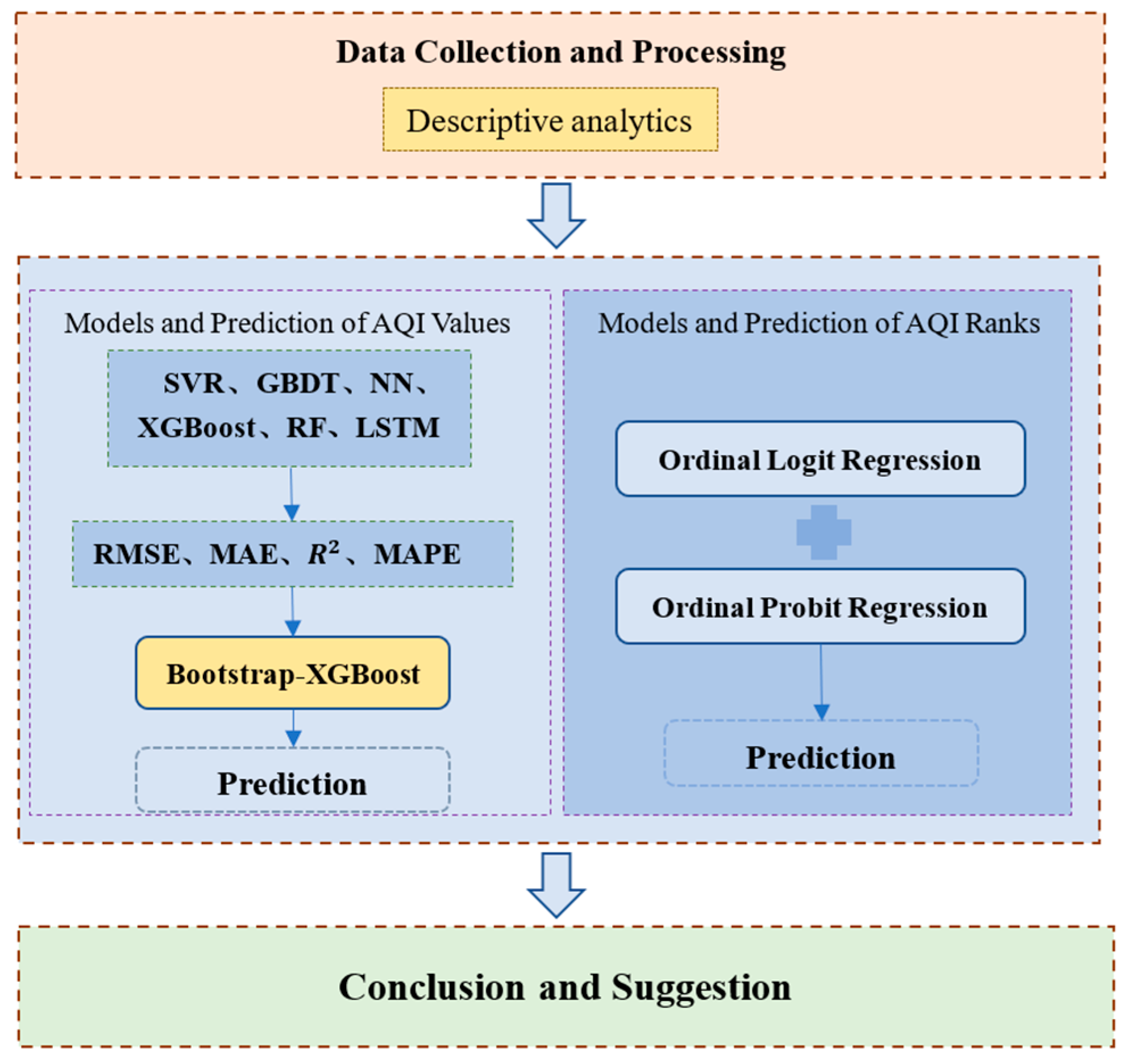
Figure 1. The research framework of this paper.
Atmosphere 15 00925 g001
Figure 2. Stacked graph of air quality shares by season.
Atmosphere 15 00925 g002
Figure 3. The flow chart of the RF algorithm.
Atmosphere 15 00925 g003
Figure 4. The illustration of NN.
Atmosphere 15 00925 g004
Figure 5. LSTM model network structure.
Atmosphere 15 00925 g005
Figure 6. The plot of predicted vs. actual AQI values on the test set.
Atmosphere 15 00925 g006
Figure 7. Box plots with 95% confidence intervals.
Atmosphere 15 00925 g007
Table 1. Basic characteristics of the data.
MinimumMaximumMeanMedianModeSkewness
AQI1343986.120667532.2285
SO24267.7342762.1754
NO289036.312332200.8220
PM2.5628352.274033172.1467
CO0.320.70470.60.61.5547
PM1010107298.66037646 and 524.6481
O3514756.372652200.5450
Table 2. Comparison of model fitting results.
ModelMAERMSEMAPE(%)R-Squared
SVR9.647233.064010.680.7611
XGBoost5.596916.13823.900.9431
GBDT9.814321.395911.40.9000
RF7.662419.24128.050.9191
CNN9.121625.80059.860.8546
LSTM6.22847.654238.110.2235
Table 3. AQI forecast values and 95% prediction intervals.
Forecast DateActual ValueForecast ValueStandard Deviation95% Prediction Interval
October 15656.81842.4194[55.0003, 64.3353]
October 22628.51792.2609[25.3514, 33.7640]
October 32523.01332.6373[22.8364, 32.3976]
October 42222.65152.6171[21.0723, 30.7458]
October 52628.01142.3195[25.0484, 33.1558]
October 62423.01332.5359[22.7003, 31.5158]
October 73633.57982.2505[32.3784, 41.1384]
October 84445.44931.9171[44.9358, 52.4214]
October 95656.81842.8158[54.9225, 64.9447]
October 107069.25842.6190[68.1752, 78.4387]
October 117777.85552.7382[77.8773, 88.8032]
October 126663.88763.2501[61.4553, 73.4492]
October 134141.75672.0295[41.7567, 48.7301]
October 143936.65772.7054[34.8364, 45.4578]
October 154041.75672.3040[40.5036, 49.5267]
Table 4. Parameter estimation results.
Ordinal Logit RegressionOrdinal Probit Regression
ParameterEstimateS.Ep-ValueEstimateS.Ep-Value
α 1 9.58261.63910.00005.48500.94730.0000
α 2 23.25163.00820.000014.01131.71840.0000
α 3 34.92704.40300.000020.75662.44140.0000
α 4 46.49495.85210.000028.02363.31410.0000
α 5 67.10618.72570.000041.20044.80890.0000
PM2.50.17290.02600.00000.11090.01460.0000
PM100.10330.01470.00000.06320.00860.0000
SO2−0.38250.14560.0086−0.24050.08930.0071
NO20.04150.02400.08340.01700.01360.2104
O30.03790.00910.00000.02240.00530.0000
CO−1.29521.66750.4373−0.94990.97230.3286
Table 5. Prediction accuracy on test set.
ModelAccuracy (%)
Ordinal logit regression model89.04
Ordinal probit regression model86.30
Table 6. Predicted results of AQI ranks.
Forecast DateTrue Rank Prediction Rank (Predicted Probability)
Ordinal Logit RegressionOrdinal Probit Regression
October 1IIII (0.6531)II (0.6729)
October 2II (0.9870)I (0.9935)
October 3II (0.9956)I (0.9994)
October 4II (0.9961)I (0.9996)
October 5II (0.9904)I (0.9966)
October 6II (0.9914)I (0.9971)
October 7II (0.9407)I (0.9493)
October 8II (0.8979)I (0.9049)
October 9IIII (0.5727)II (0.5560)
October 10IIII (0.9978)II (0.9999)
October 11IIII (0.9923)II (0.9989)
October 12IIII (0.9974)II (0.9999)
October 13II (0.9157)I (0.9213)
October 14II (0.9159)I (0.9258)
October 15II (0.9078)I (0.9249)
Disclaimer/Publisher’s Note: The statements, opinions and data contained in all publications are solely those of the individual author(s) and contributor(s) and not of MDPI and/or the editor(s). MDPI and/or the editor(s) disclaim responsibility for any injury to people or property resulting from any ideas, methods, instructions or products referred to in the content.