Abstract
This study investigates how urban environments influence boundary layer processes during the passage of a Great Salt Lake breeze using a multi-scale modeling system, NCAR’s WRF-Coupled GPU-accelerated FastEddy® (FE) model. Motivated by the need for sub-10 m scale decision support tools for uncrewed aerial systems (UAS), the FE model was used to simulate turbulent flows around urban structures at 5 m horizontal resolution with a 9 km × 9 km domain centered on the Salt Lake City International Airport. FE was one-way nested within a 1 km resolution Weather Research and Forecasting (WRF) domain spanning 400 × 400 km. Focused on the late morning lake breeze on 3 June 2022, an FE simulation was compared with WRF outputs and validated using surface and radar observations. The FE simulation revealed low sensible heat flux and cool near-surface temperatures, attributed to a relatively low specification of thermal roughness suitable for previously tested FE applications. Lake breeze characteristics were minimally affected, as FE effectively resolved interactions between the lake breeze and urban-induced turbulent eddies, providing insights into fine-scale boundary layer processes. FE’s GPU acceleration ensured efficient simulations, underscoring its potential for aiding decision support in UAS operations in complex urban environments.
1. Introduction
Uncrewed aerial systems (UAS) will increasingly rely on high-resolution weather models to resolve the potential impacts of boundary layer turbulence on flight operations [1]. UAS studies suggest that turbulence at sub-meter to meter scales significantly affects UAS flights [2,3]. The resolution of operational numerical weather prediction (NWP) models at national centers has increased dramatically, with resolutions now approaching ~1 km [4]. The High-Resolution Rapid Refresh (HRRR) model with Δ = 3 km horizontal grid spacing is the highest-resolution operational NWP model covering the contiguous United States [5,6]. However, this grid spacing is too coarse to provide UAS operators with sufficiently detailed urban wind estimates. The sub-km scales necessary to resolve critical boundary layer circulations are often referred to as operational NWP’s “terra incognita” or “grey zone” [7,8]. When mesoscale model grid spacing is less than the largest thermal eddies (~1 km), boundary layer scale turbulence is often filtered out by fully parametrizing turbulent scale transfer [9,10]. Planetary boundary layer parameterizations struggle to estimate average turbulent eddy behavior [11].
Many techniques are available to downscale operational NWP model winds to horizontal grid spacings of O(1 km) or less in complex terrain and urban areas, e.g., mass-conserving approaches that help the development of parameterizations for coarser resolution NWP models [12,13,14,15,16]. The HRRR and other operational models are often used to initialize models such as the Weather Research and Forecasting (WRF) model with embedded nests at large eddy simulation (LES) scales potentially advantageous for UAS operations and urban modeling [11,17,18,19,20]. For example, the HRRR was utilized in a previous study to initialize a WRF-LES simulation with a 111 m horizontal resolution for operational UAS decision support during the 2018 LAPSE-RATE experiment [17]. However, output from the simulation was not available until 18 hours after the initialization time.
Although utilizing LES at sub-100 m resolution is possible, Central Processing Unit (CPU)-based LES codes at those scales are computationally expensive and time-consuming. The National Center for Atmospheric Research (NCAR) has developed the NCAR Graphics Processing Unit (GPU)-accelerated LES FastEddy (FE) model, leveraging GPU-based LES for accelerated simulations [21]. The current generation of NVIDIA GPUs (Tesla V100 GPUs) was shown to speed up simulation times by a factor of 6.0, such that 1 GPU is equivalent to 256 CPUs [21,22]. One-way coupled meso- to microscale simulations have demonstrated FE’s ability to diagnose diurnal variations in wind and turbulence with good agreement relative to observations [23,24].
In urban regions, highly complex flow fields characterized by turbulent mixing of mass, heat, and moisture prevail throughout the boundary layer. LES models, such as FE, explicitly resolve prognostic fields at their specified horizontal and vertical length scales and rely on turbulence closure parameterizations at finer scales. LES models implement scale separation using low-pass filters (i.e., convolution filters [25]) to retain low frequencies (large eddies) while attenuating high-frequency signals (small eddies) that are parameterized using sub-filter scale stress terms. FE uses several stress tensor parameterizations derived on work from Lilly [26,27].
Simulations in Dallas, TX by Muñoz-Esparza et al. [23,24] illustrate the FE model’s ability to simulate turbulent flows in the street canyons of a major metropolitan center. UAS operations worldwide are likely to be undertaken in highly variable mixes of residential and commercial areas under wide-ranging meteorological conditions. UAS flights can be expected from major distribution centers near rail and air transportation hubs and final destination delivery staging areas within small business or residential areas. Current operational models at horizontal resolutions of O(3 km) may be useful to alert UAS operators when wind speeds are likely to exceed 10 m s−1 that affect flight paths and the stability of lighter UAS [28,29]. However, convection, terrain-flow interactions, or surface heating during weaker flow periods may lead to small-scale spatially heterogeneous winds and turbulence that have the potential to further complicate UAS flight operations and which are parameterized, but not well captured, by mesoscale models.
Summer lake breezes typically require Air Traffic Control at the Salt Lake City (SLC) International Airport to switch incoming flights during late morning from landing from the north to landing from the south [30]. The nocturnal and early morning southerly winds “down” the Salt Lake Valley shift to northwesterly winds “up” the Valley as a response to the increased surface heating in the Valley relative to the nearby Great Salt Lake (GSL) [31,32]. Occasionally, a highly turbulent lake breeze front develops at the leading edge of the breeze, although the ambient horizontal wind speeds may remain below the criteria expected to curtail UAS operations [33].
The objective of this study is to examine an FE model simulation during the passage of a weak lake breeze front that progressed across the SLC International Airport on 3 June 2022. Prior FE simulations have focused on situations with stronger mesoscale dynamical forcing in which surface heating plays a secondary role. The summer lake breeze front provides a distinctive progressive meteorological signal that interacts in complex yet relatively well understood ways with other terrain-forced circulations, buildings, and strong surface heating across heterogeneous land-surface types. This study aims to establish a foundational understanding of model performance and challenges associated with utilizing FE in arid complex terrain. A subsequent study will examine the model’s sensitivity to the presence of buildings and the intensity of surface heating. Section 2 provides a detailed overview of the model setup. Section 3 presents the results, focusing on the complex interactions between urban environments and boundary layer processes using the FE model. Section 4 presents a discussion and summary of the results, along with outlining future research. These future studies will conduct a detailed sensitivity analysis to assess the impact of various parameters, such as the removal of buildings, adjustments to internal building temperatures, and modifications to thermal surface roughness. These efforts aim to clarify uncertainties and enhance the reliability of FE model results in urban environments.
2. WRF and FastEddy Model Configuration
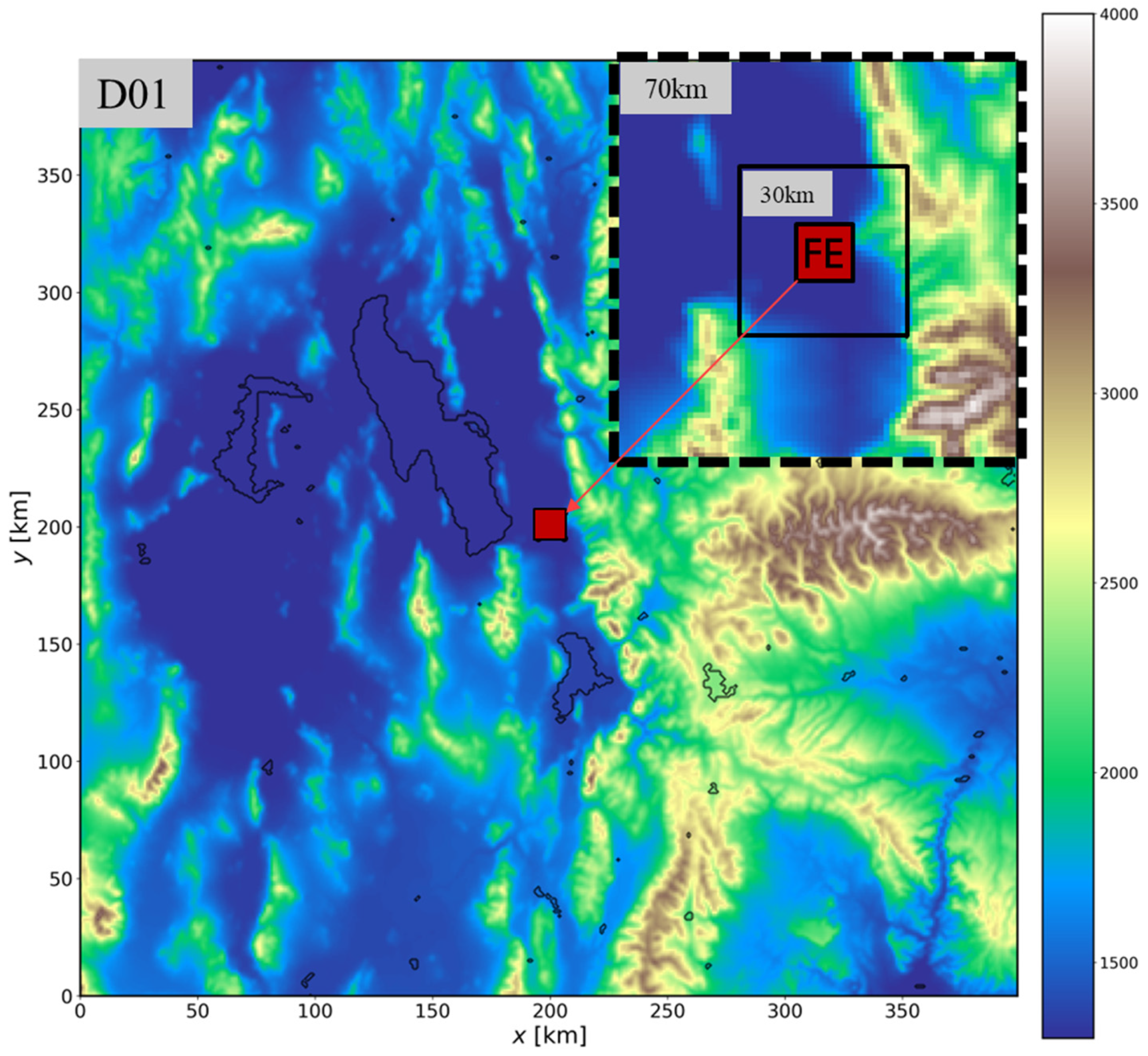
HRRR hourly analyses beginning at 00:00 UTC 3 June 2022 were used to initialize and provide boundary conditions for a 1 km horizontal resolution WRF [34] 24 h simulation over a 400 × 400 km domain centered on the SLC International Airport (Figure 1). The overestimated spatial extent of the GSL in the default WRF land use field was modified to conform to the lake’s areal extent during 2022 as shown in Figure 1. The WRF lake depth, land use category, and soil top and bottom values in the WRF geogrid file were also adjusted similar to the changes made by Blaylock et al. [33]. Other details regarding the WRF simulation are shown in Table 1. Urban physics parameterization schemes available in WRF (e.g., single-layer urban canopy model, Kusaka et al. [35] or building effect parametrizations, Martilli et al. [36]) use the Noah land surface model as a foundation with additional urban-induced latent and sensible heat and fraction coverage of urban surface term added to estimate the total grid-scale sensible heat flux [37]. Urban physics parameterizations, like those available in WRF, were not used in this study since the specific parameters to characterize buildings required to use them had been developed for other locations [13,38,39,40,41] and are not available for Salt Lake City. WRF Δ = 1 km resolution simulations run by us for a Chicago, IL, domain revealed minimal differences in wind and temperature between the simulations with and without urban physics parameterizations.

Figure 1.
WRF 1 km domain with terrain elevation shaded according to the colorbar. The red shaded box delineates the FE domain. The dashed-bounded inset shifts and expands the 1 km WRF grid in order to view the FE domain and 30 km WRF subdomain shown in later figures.

Table 1.
WRF and FE configuration details.
The FE simulations are initialized at 14:00 UTC (7:00 LST) 3 June 2022 and forced on the FE’s boundaries over the subsequent 5 h by the WRF simulation. The FE domain is an 81 km2 square region discretized using (Nz, Ny, Nx) = (1794, 1782, 122) grid points with a grid spacing of Δx,y = 5 m horizontally. Thus, the FE domain is comprised of ~400 million grid points and is ~0.05% of the WRF domain. (For reference, the current operational HRRR model uses 1799 × 1059 grid points and 52 vertical levels for a total of ~100 million grid points to cover the entire CONUS.) The vertical grid spacing in the terrain-following grid gradually expands as altitude increases to ~3600 m AGL to allow for boundary layer growth. Details regarding FE are available in the studies by Muñoz-Esparza et al. [22,23,24], and the Open Source version of FE is described online [42]. FE was run on NCAR’s high-performance computing system, Derecho, at the Wyoming Super Computing Center in Cheyenne, WY [43]. Each 5 h FE simulation (14:00–19:00 UTC 3 June) required 18 h across 64 GPUs (16 GPU nodes) on Derecho. Dozens of these simulations were made for testing and development, of which only one is described here. The FE simulation uses prescribed lateral, bottom, and top boundary conditions from the WRF simulation. The cell perturbation method described by Muñoz-Esparza et al. [44,45] introduces finite amplitude perturbations to the potential temperature perturbations near and along the inflow boundaries that are dynamically updated based on the WRF’s lateral boundary conditions. This method accelerates the generation and development of turbulence. To achieve full development and equilibrium of turbulence in regions of interest, a 1 km fetch from the boundary is imposed, which is less than that required for other methods [46,47].
As shown in Table 1, the FE simulations do not explicitly consider radiative effects and instead are forced by time-dependent surface boundary conditions (e.g., skin temperature and water vapor) that are ingested by the FE’s Monin–Obukhov Similarity Theory (MOST) surface layer scheme. The MOST approach computes friction velocities and exchange coefficients for surface heat and moisture fluxes in land surface models (LSM), using momentum roughness from the NLCD reference list and user-prescribed thermal roughness, feeding into the Noah LSM bulk heat transfer equation to compute sensible heat flux. Hence, these FE simulations do not consider the urban canopy energy budget and sensible and latent heat fluxes generated by buildings. Additional details on the FE model configuration are further described in previous studies [21,24].
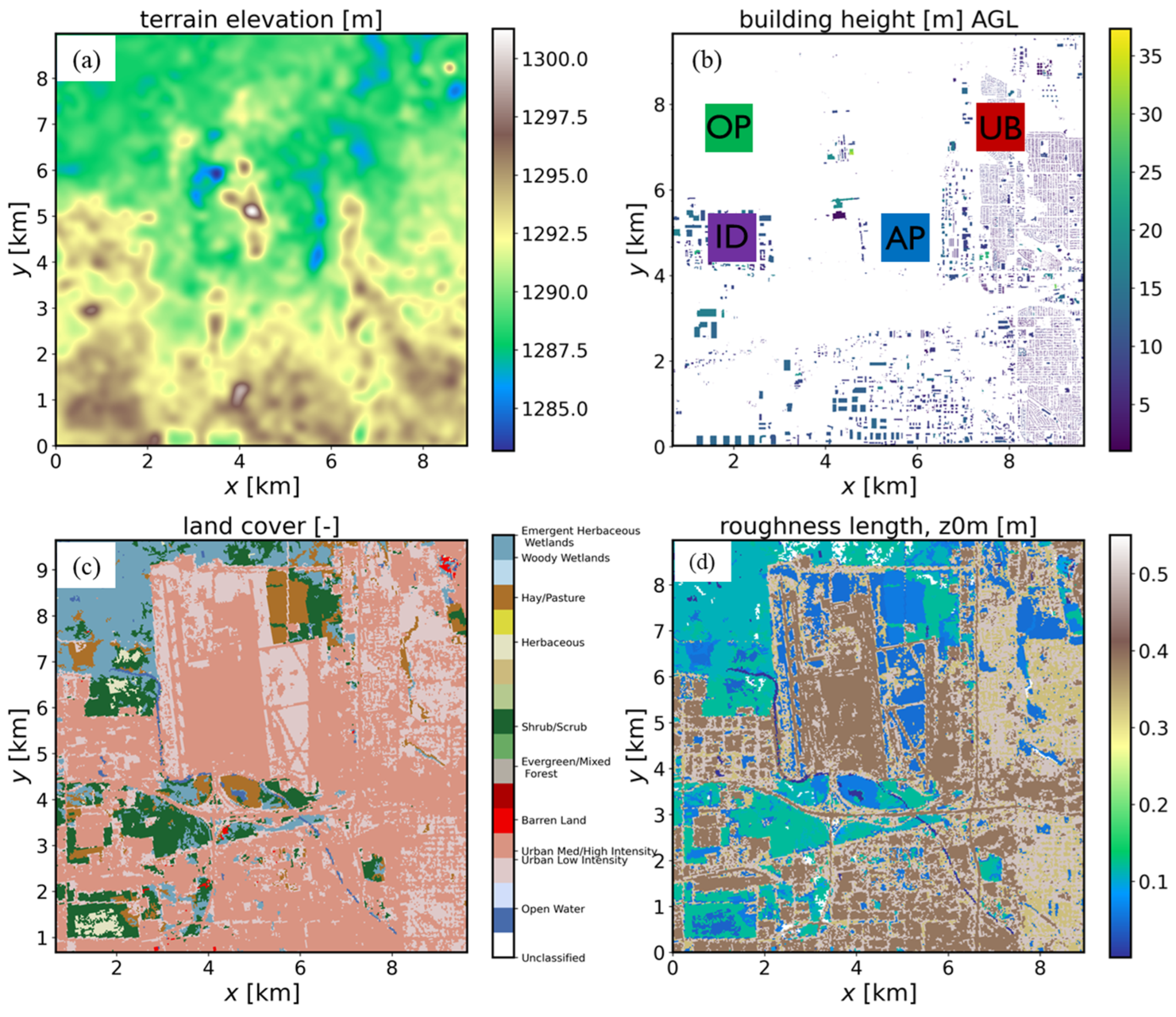
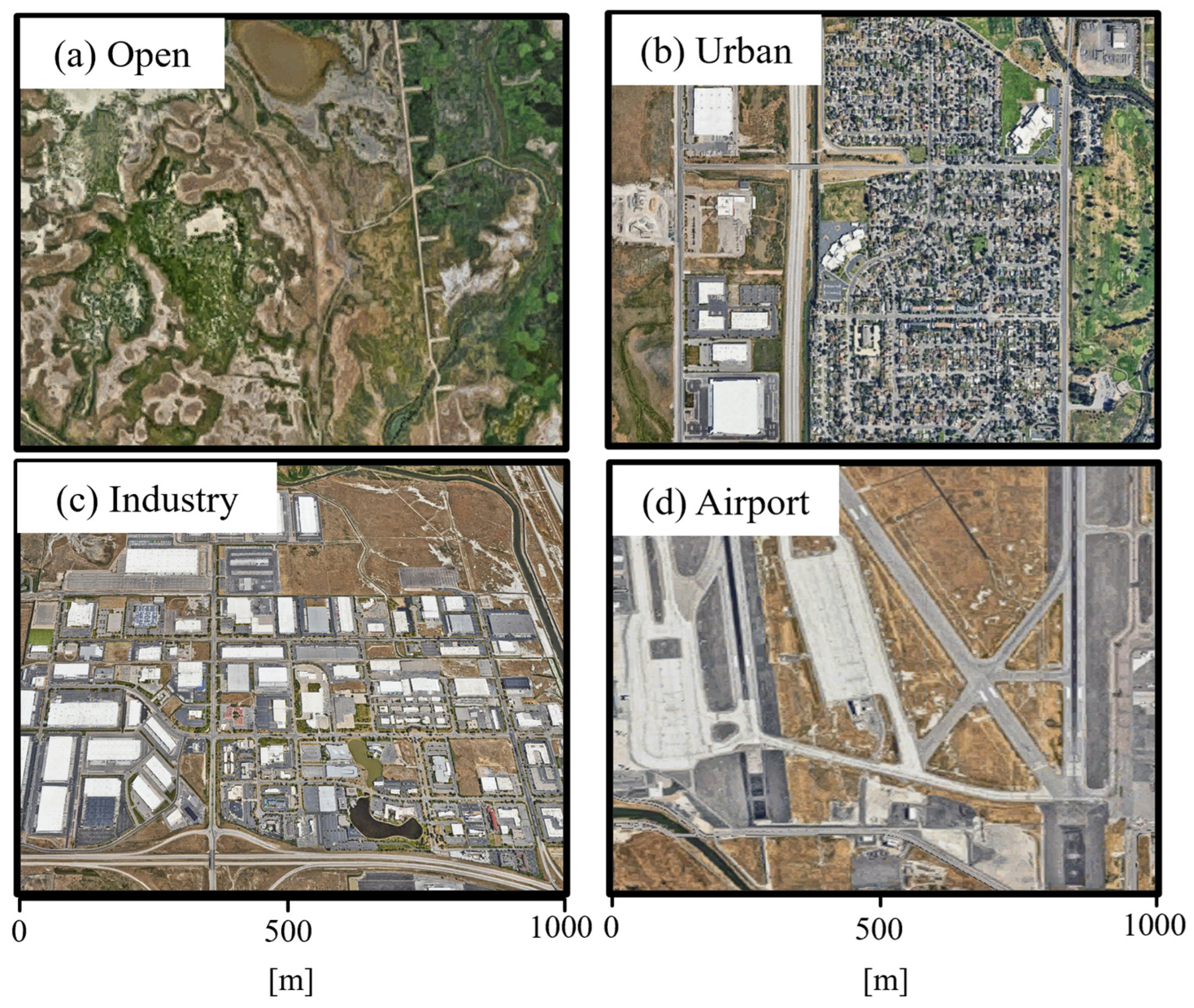
Figure 2 illustrates the terrain, land cover, building locations, and roughness length within the FE domain. A building mask was developed for the FE domain using ArcGIS Pro software to extract building height, size, elevation, and location from the USGS LPC UT Wasatch L4 2013 LAS 2016 Lidar dataset [48]. The Lidar dataset was subset into categories such as ground elevation, vegetation, and buildings. The ground elevation subset was used to create a digital terrain model (DTM), which is simply the elevation of the bare surface after minor smoothing to limit model instabilities. When comparing Figure 2a to Figure 1, very slight elevation gradients are evident across the FE domain. The DTM terrain was subtracted from a digital surface model (DSM) comprising the ground elevation and building subsets to extract building height (Figure 2b). The exact location and shape of the buildings were verified relative to 2018 building footprints from the Utah Geospatial Resource Center [49]. Structures with high root mean squared error (>2 m) were manually adjusted to match the building footprint. Between 2016 and 2022, most of the buildings remained unchanged, except that manual adjustments were necessary to reflect major upgrades to the airport during this period. As shown in Figure 2c, the 2016 USGS National Land Cover Database land cover and use were also processed for the FE domain. Following the same land cover to roughness conversion table used in WRF, land cover was used to assign to each grid point prescribed roughness length values, as shown in Figure 2d. These input grids were transformed to the WRF’s Lambert Conformal projection at 1 m resolution centered on the SLC Airport within the FE domain. The colored 1 × 1 km squares in Figure 2b define four representative subdomains shown in Figure 3: Open (OP), primarily shrub and grasslands with low roughness; Industrial (IP), large structures typically housing commercial distribution facilities near the airport; Airport (AP), open runway area within the airport facility with low roughness; and Urban (UB), small residential and commercial buildings.
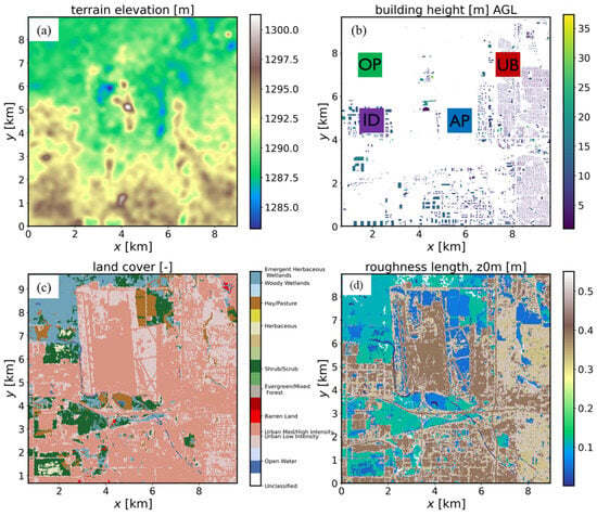
Figure 2.
(a) FE model terrain (m); (b) building height (m); (c) land cover type; and (d) roughness length (m).
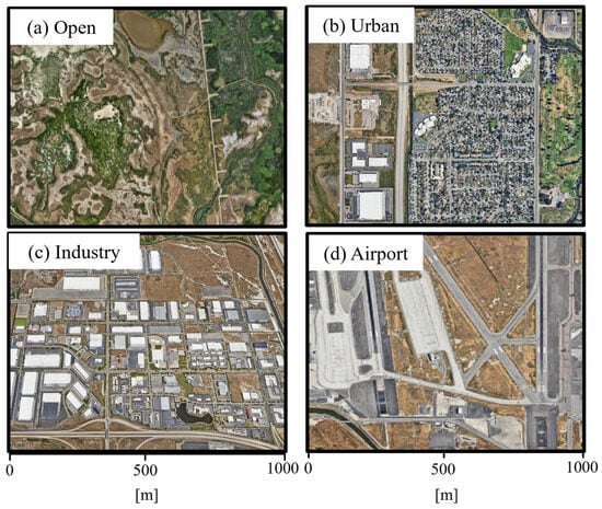
Figure 3.
FE 1 × 1 km subdomains: (a) Open; (b) Urban; (c) Industry; and (d) Airport.
FE uses a scale-independent version of the Chan and Leach [50] immersed body force method (IBFM), adding increased drag forces to the momentum equations at building grid points. IBFM slows flow approaching buildings, similar to fluids encountering solid objects, and no flow is possible through a building grid point. The scale independence of the IBFM allows for the modeling of solid bodies at any grid size (Muñoz-Esparza et al. [23]). Shin et al. [51] suggest that building-induced flow responses become less important when the turbulence scale becomes larger than the building size. As evident in Figure 2b and Table 2, the average height and size of the 20,607 buildings in our domain are relatively small since most are residences and small commercial buildings. (The building maxima reflects the height of the Air Traffic Control Tower and the primary airport structure’s spatial footprint.) Although the direct impact of any individual building may be relatively small, the cumulative effect of all of these buildings may be large and depend on how they are arranged across the landscape.

Table 2.
FE domain building characteristics for the 20,607 buildings.
Zero wind speed and constant temperature and moisture are specified inside building-masked volumes to minimize momentum, energy, and mass exchange between the buildings and the environment. Shin et al. [51] note that the extended IBFM does not entirely eliminate such exchanges arising from advection and diffusion through building walls. Since prior FE studies have focused primarily on dynamically forced flows across major urban centers with buildings of sizeable areal extent, such exchanges were less evident than we found in this study. The configuration of this FE simulation did not include a building model. Hence, there is no accounting for the impacts of building radiative effects on sensible heat fluxes. Our initial FE simulations assumed the initial temperature inside building-masked grid volumes (20 °C at 14:00 UTC) remained constant throughout the simulation while the outside air temperature increased to over 28 °C by 19:00 UTC. For the simulation investigated in depth in this study, the internal building temperatures are set to the time-evolving mean WRF-provided lateral boundary profiles. Since buildings that are close to or smaller than the horizontal resolution are unresolved, internal building temperatures may be advected into the surrounding environment. Such impacts of building interior temperatures on the FE simulations will be presented in a later study. Additional sensitivity experiments will be presented in that study that examine removing all buildings and varying the thermal roughness length (z0h) that, along with surface temperature, wind speed, and stability, controls the intensity of surface heat flux. As discussed by Mahrt [52], z0h is challenging to parameterize and is quite variable but is typically assumed to be related to, but smaller than, the aerodynamic surface roughness length (z0m). Previous studies examined six such parameterizations for a land–atmosphere model and illustrated that high values of z0h lead to overestimates of sensible heat flux [53,54,55]. The simulation presented here sets z0h to 0.1 of z0m, which has been used in the default setup for other FE simulations.
3. Results and Discussion
Observations and Simulations of Lake Breeze Frontal Passage
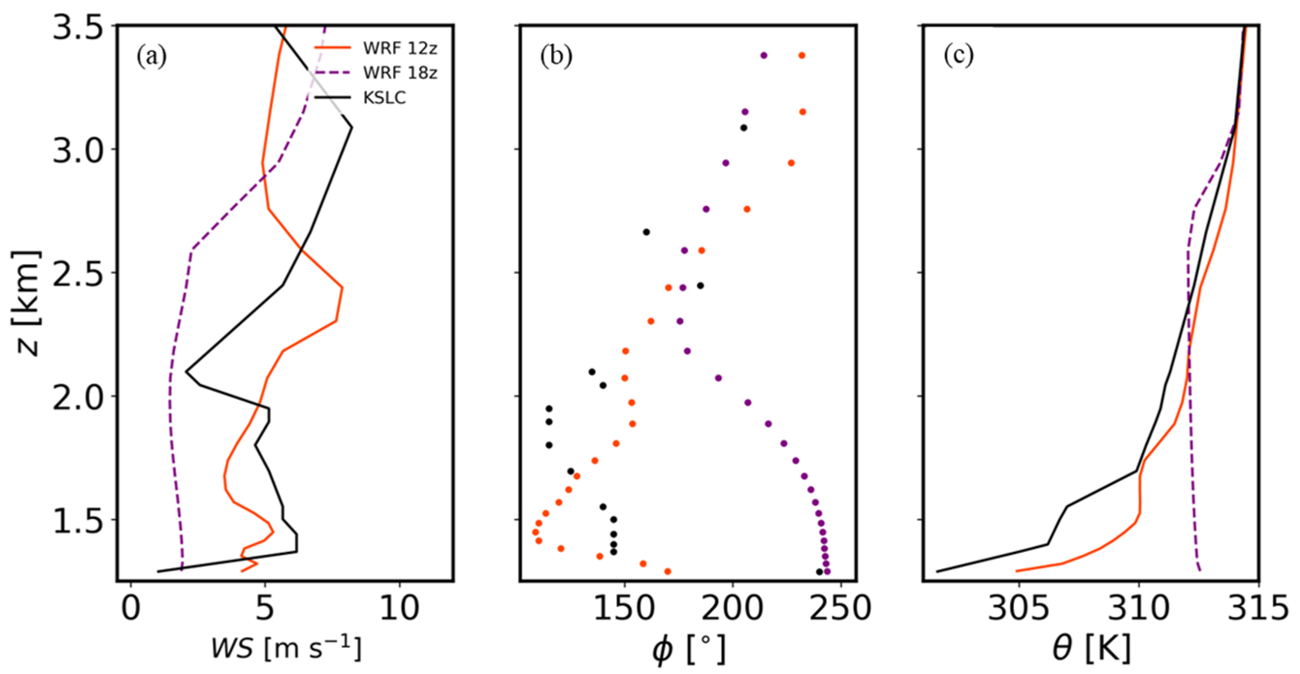
The western United States on 3 June 2022 was dominated by a north–south-oriented ridge at 500 hPa extending from eastern Utah to Alberta, Canada. The 12:00 UTC (5:00 LST) sounding launched from the SLC International Airport indicated clear skies with 6 m s−1 southeasterly down-valley winds near the surface that weakened through the lowest 700 m AGL (Figure 4a). The southeasterly near-surface winds were embedded within a strong stable layer arising from nocturnal radiational cooling (Figure 4c). The WRF simulation valid at 12:00 UTC has comparable vertical profiles of wind speed and direction in the boundary layer near the SLC International Airport. However, the WRF potential temperature in the lowest 300 m is ~3–4 K higher than observed (Figure 4c). Over the next 6 h, surface heating in the WRF simulation mixes out the near-surface stable layer and develops an approximately adiabatic profile within the lowest 1500 m. Light southwesterly winds reflect the prefrontal conditions (Figure 4b).
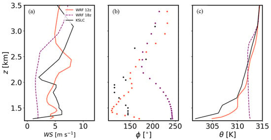
Figure 4.
Observed vertical profiles (MSL) at KSLC (black) at 12:00 UTC (05:00 LST) 3 June 2022 of: (a) wind speed; (b) wind direction; and (c) potential temperature (θ). WRF-simulated profiles shown in each panel for 12:00 UTC (red) and 18:00 UTC (purple).
Meteorological data are available from six surface stations inside the FE domain, with over a hundred stations across the area shown in Figure 5. Between 14:00 and 16:00 UTC, stations within the FE domain and most of the northern end of the SLV continued to experience southeasterly light winds, consistent with the earlier sounding. Southerly winds increased to 3–4 m s−1 between 16:00 and 17:00 UTC as down-valley flow extended northward. The distinctive passage of the lake breeze front at the airport was evident between 17:50 and 17:55 UTC by a shift to northwesterly winds, a wind speed increase to 5–6 m s−1, and a dewpoint temperature increase of 3 K. As documented by Zumpfe and Horel [30] for other lake breeze fronts, only a slight drop in temperature typically follows their passage due to the continued surface heating in this arid environment during summer.
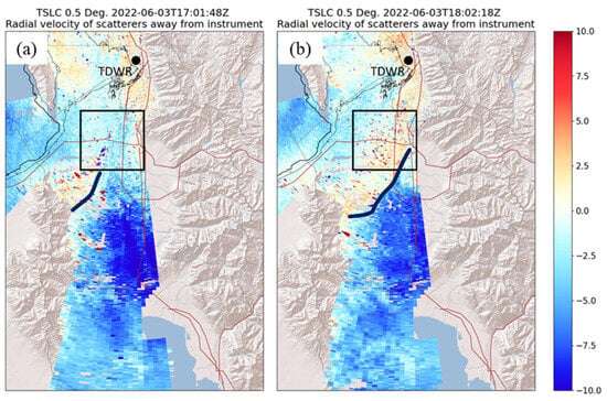
Figure 5.
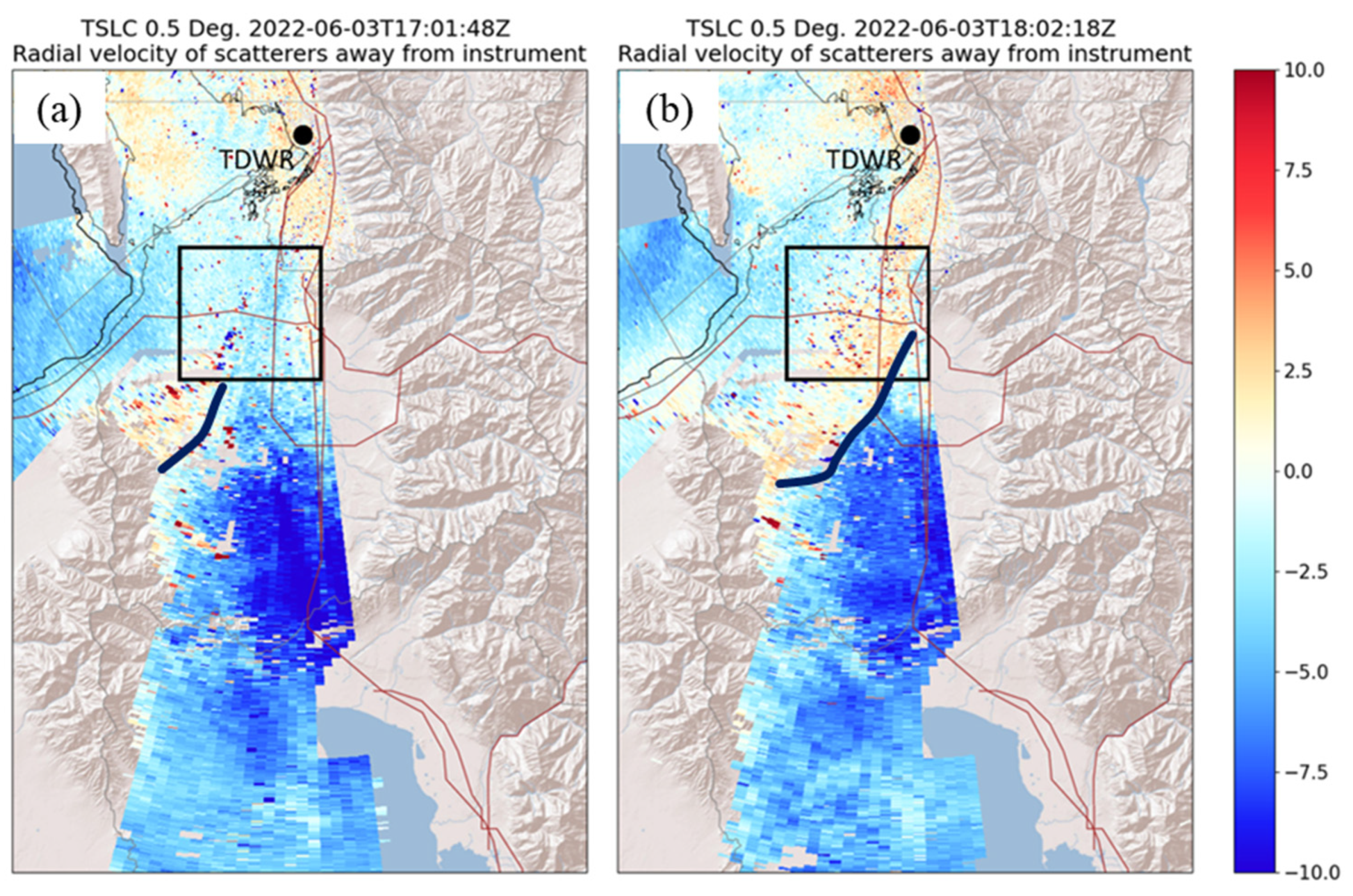
Plan view 0.5◦ radial wind speed (m s−1) from TSLC radar (black dot) for (a) 17:01 UTC 3 June 2022 and (b) 18:02 UTC 3 June 2022. Blue (orange) shading denotes flow toward (away) from the radar. The black box indicates the FE domain. The blue line denotes the position of the lake breeze front.
Radial wind observations are available from the TSLC Terminal Doppler Weather Radar located on the valley floor ~20 km north-northeast of the SLC International Airport (Figure 5). At 17:00 UTC (Figure 5a), the 0.5° elevation angle radial wind speeds are dominated by down-valley (southerly) wind with lighter southerly winds within the FE domain. Based on surface observations and the radial winds in Figure 5a, the lake breeze front pushed preferentially into the northeast corner of the Salt Lake Valley, since that region is adjacent to the GSL’s open water. By 18:00 UTC (Figure 5b), the lake breeze had crossed nearly all of the FE domain, as evidenced by the outbound radial winds behind the front. The weak inbound speeds further behind the front result from a shift from northwesterly to westerly winds by that time.
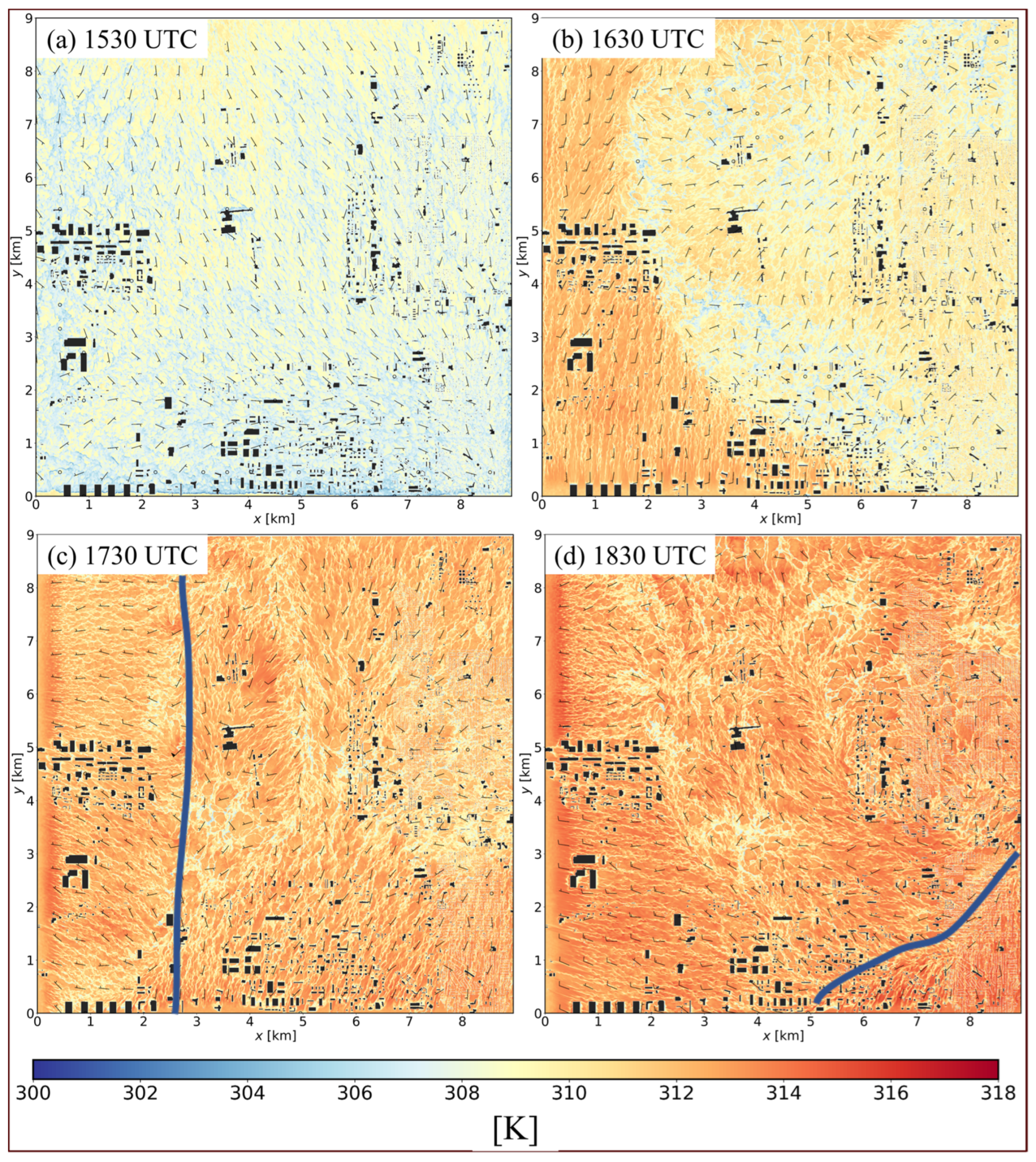
Figure 6 illustrates the temporal evolution of WRF 2 m potential temperature (θ) and 10 m winds within the 30 km inset outlined in Figure 1. At 15:30 UTC (08:30 LST, Figure 6a), the WRF wind field is characterized by 1–4 m s−1 southerly winds with θ ~309–310 K. One hour later (Figure 6b), surface heating during the morning and stronger southerly down-valley flow across the western sector of the FE domain leads to higher θ there. The influence of the lower lake temperature (19 °C) is evident by the lower θ and westerly–northwesterly flows preferentially pushing towards the southwest of the FE domain. The increased southerly winds to the west of the FE domain slowed the lake breeze’s eastward progression. By 17:30 UTC (10:30 LST), the lake breeze front enters the western FE domain, characterized by westerly to northwesterly flow and wind speeds between 1 and 4 m s−1 (Figure 6c). The WRF simulation indicates a slower progression of the lake breeze front through the FE domain, with the front crossing the Airport region by 18:30 UTC instead of that observed (17:55 UTC).
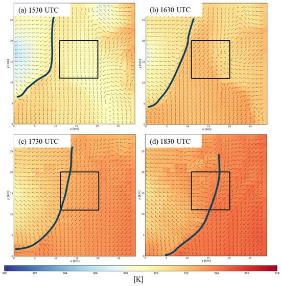
Figure 6.
WRF 10 m wind barbs and 2 m θ within the 30 km domain shown in Figure 1 at: (a) 15:30 UTC; (b) 16:30 UTC; (c) 17:30 UTC); and (d) 18:30 UTC. Wind speeds of 1 m s−1 (5 m s−1) are denoted by half (full) barbs. The black box outlines the FE domain. The heavy blue line indicates the location of the lake breeze front.
For comparison to the output from the WRF simulation, Figure 7 shows θ at every grid point and 10 m winds plotted at every 100th grid point from the FE simulation. After the FE simulation evolves over the first 1.5 h (15:30 UTC, Figure 7a), the FE environment is characterized by 1 to 4 m s−1 southeasterly flow and θ values 4 K lower than WRF. By 16:30 UTC (Figure 7b), surface heating and down-valley flow result in higher θ along the western edge of the domain with fine-scale turbulent features evident in the θ field. The FE simulation develops northeasterly winds and sustains lower θ in the eastern half of the domain that was not observed or simulated by WRF. This anomalous pool of lower θ is exacerbated initially by weak easterly winds across the eastern boundary (Figure 6a) and, as will be shown later, maintained by underestimated surface sensible heat fluxes in this region.
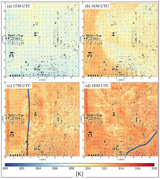
By 17:30 UTC (Figure 7c), the lake breeze front was advancing across the western third of the domain, the timing of which was influenced by the evolving boundary conditions imposed by the WRF simulation. Note that θ along the western boundary imposed by the WRF at this time is higher than that simulated further inside the FE domain. Stronger turbulence is evident by the θ streaks in both the prefrontal southerly flow and postfrontal westerly flow. Light and variable winds persist over the residential area east of the airport. The lake breeze front simulated by FE progresses faster across the domain than WRF (compare Figure 6d and Figure 7d). FE’s faster frontal speed may have resulted from the weaker flows opposing its progression across the domain. The lower θ in the FE simulation relative to WRF continues, as evident by the FE’s “warm” streak imposed along the western boundary, with turbulent streaks resulting from flow interactions with structures throughout the model domain.
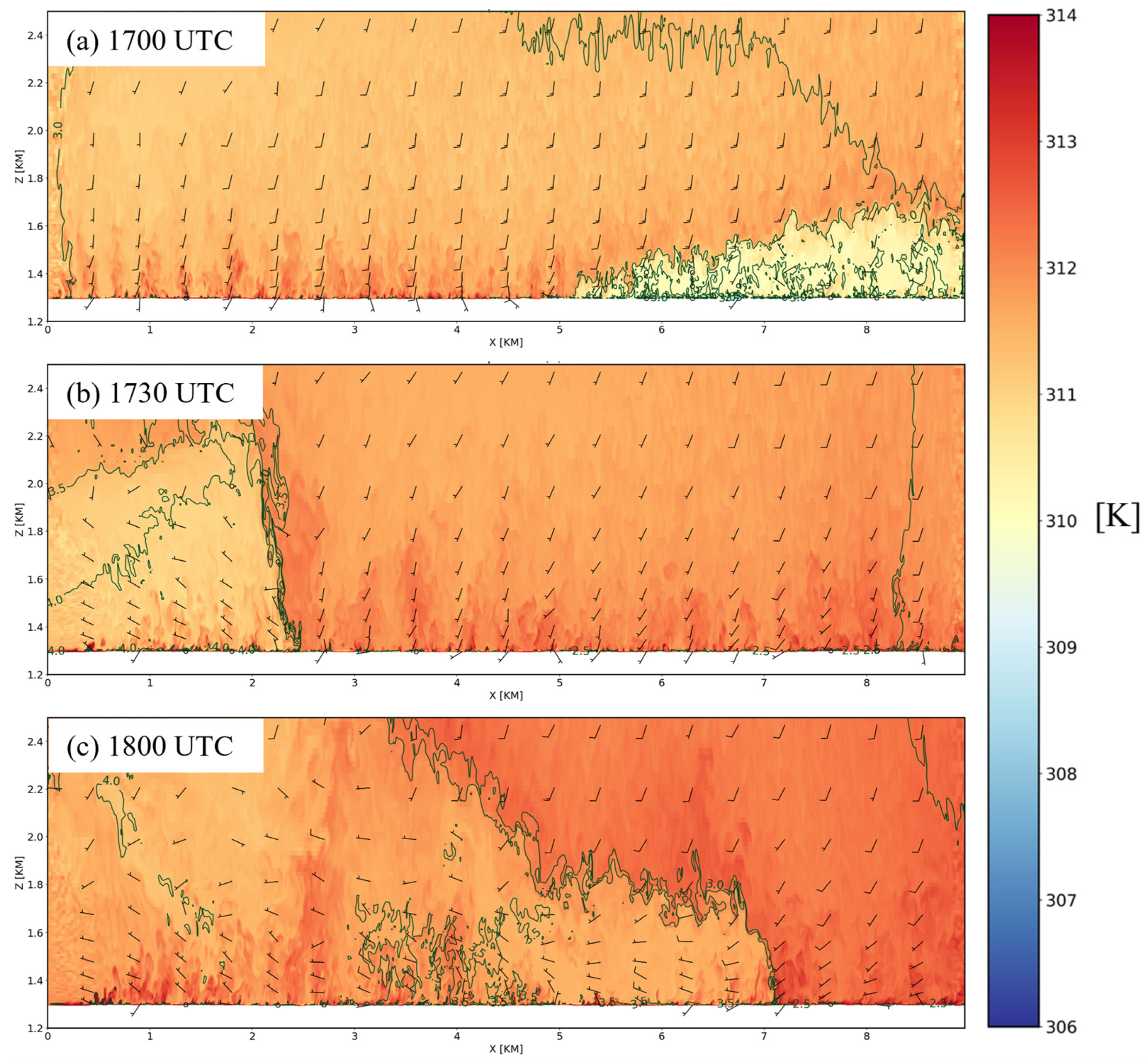
Figure 8 illustrates the WRF-simulated vertical structure and progression of the lake breeze within the east–west cross-section outlined in Figure 7a. At 17:00 UTC (10:00 LST), a well-mixed adiabatic environment is evident across the domain. As surface heating imposed by the WRF skin temperature increases during this hour, θ increases by several K throughout the boundary layer ahead of the lake breeze. The simulated lake breeze’s slower than observed eastward progression is evident by the wind shift to northwesterly flow, slightly lower θ, and increases in mixing ratio to 3.5–4.0 g kg−1.
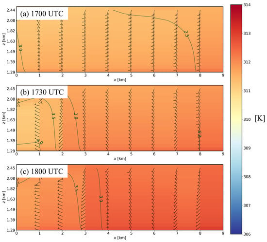
Figure 8.
WRF θ along the Y = 2 km east–west cross-section denoted in Figure 7a (shading in K), mixing ratio (green contours in g kg−1), and 10 m horizontal wind vectors at: (a) 17:00 UTC; (b) 17:30 UTC; and (c) 18:00 UTC. Wind speeds of 1 m s−1 (5 m s−1) are denoted by half (full) barbs.
The lake breeze structure simulated by FE within the east–west cross-section is shown in Figure 9. At 17:00 UTC (10:00 LST), the morning stable layer persisted over the eastern sector with 2 K lower θ compared to those aloft and within the well-mixed adiabatic environment across the rest of the domain. The surface heating imposed by the WRF skin temperature wherever buildings are absent contributed to buoyant thermal plumes rising in the western portion of the domain, while plumes and rising motion are much weaker within the eastern stable layer. Mixing ratios within the stable layer ranged from 3 to 3.5 g kg−1 in contrast to ~2.5 g kg−1 in nearly all of the rest of the cross-section. As will be shown later, the lower near-surface θ in the eastern sector may result from weaker surface sensible heat fluxes in this region despite the imposed higher WRF-imposed skin temperatures.

Figure 9.
As in Figure 8, except for the FE simulation with every 100th horizontal wind vector plotted, at (a) 1700 UTC, (b) 1730 UTC, and (c) 1800 UTC.
By 17:30 UTC (Figure 9b), the stable layer mixes out due to continued surface heating and buoyant thermals extend upwards across much of the domain in advance of the lake breeze front. The pronounced lake breeze front’s head [30,33] extends upwards ~900 m, evident in the sharp horizontal gradients in θ and the mixing ratio between 2 and 2.5 km. A turbulent plume of higher θ extends upwards immediately ahead of the front as a result of upward vertical motion exceeding 3 m s−1. Behind the lake breeze front, θ is 1–2 K lower, winds shift to westerly at 1–4 m s−1, and the mixing ratio transitions rapidly from 2.5 to 4 g kg−1.
The front progresses eastward at a speed of ~2.5 m s−1 during the next 30 min, which is consistent with the advective speed of FE’s westerly component of the postfrontal flow (Figure 9c). The front’s head decreases in depth, the leading upward wind speeds drop to ~1 m s−1, and the gradients in θ and mixing ratio across the front weaken during this period. The weakening of the front as it progressed across the domain is likely strongly influenced by the ongoing surface heating imposed by the WRF skin temperature boundary condition wherever buildings are not present.
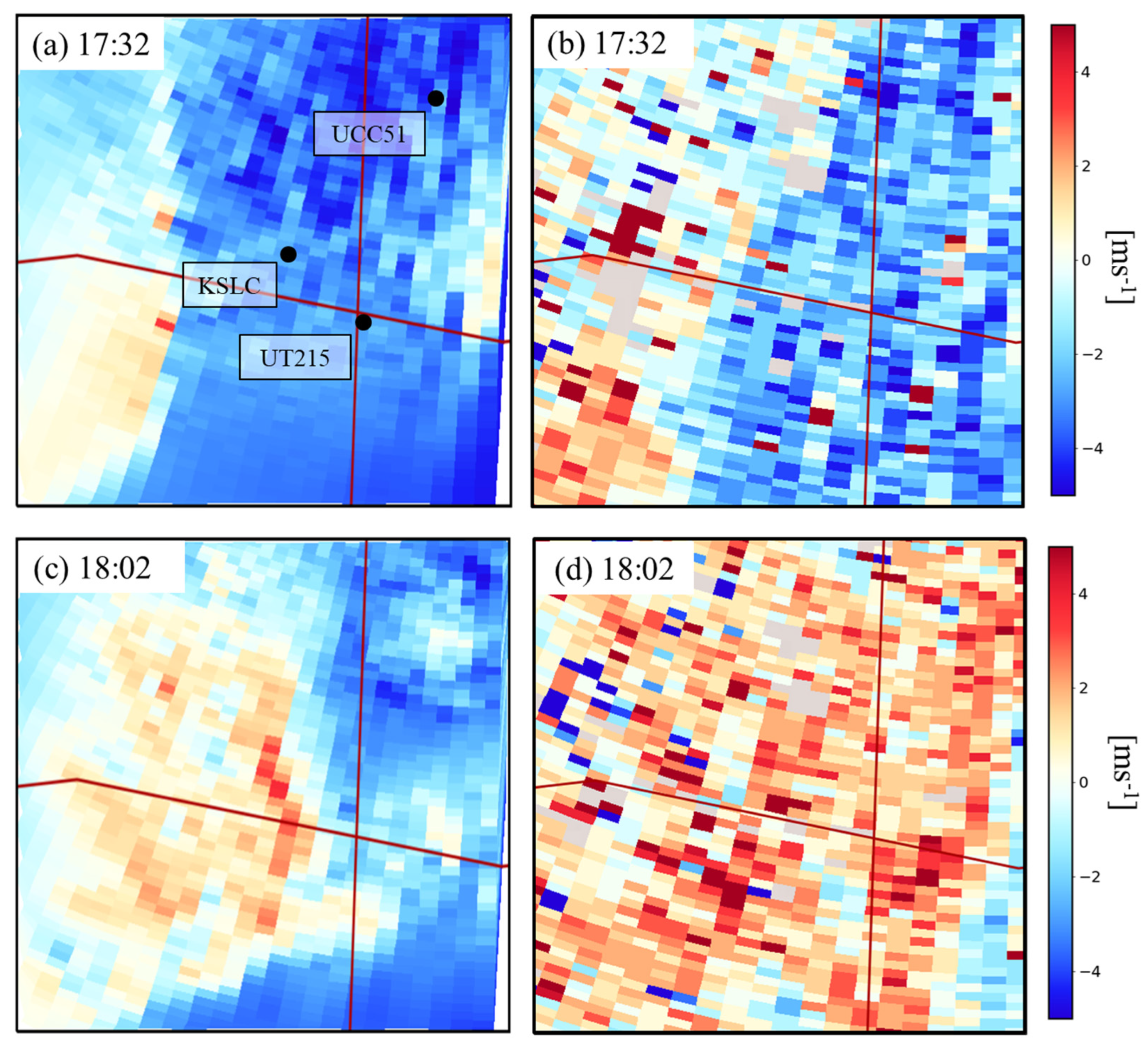
5 m resolution FE winds are mapped in Figure 10 to the TSLC radar’s polar coordinate 0.5° elevation angle radial wind reference frame. That transformation of the three-dimensional FE wind field enables validating the FE winds relative to those observed from the TSLC radar. While the observed radial scans contain clutter from vehicles and aircraft, the dominant signal at 17:32 UTC (Figure 10a) is inbound (southerly) winds ahead of the front and outbound or weak inbound speeds behind it. By 18:02 UTC (Figure 10b), the front is evident only in the extreme southeast corner of the figure’s domain, with more substantial outbound velocities in its wake. The FE simulation captures the general sense of the progression of the lake breeze front across the domain (Figure 10a,c). However, the slower eastward speed of the front in the WRF simulation affects details in the FE simulation. For example, the continued inbound flow at 18:02 UTC imposed by WRF on the southern boundary impedes frontal progression in that area with more rapid frontal movement near the airport and along the I-80 corridor (i.e., the east–west-oriented red line in Figure 10c).

Figure 10.
Radial wind speed at 0.5° elevation angle within the FE 9 km × 9 km domain according to the colorbar: (a) FE-simulated speeds at 17:32 UTC; (b) as in (a) except for TSLC-observed speeds; (c) as in (a) except at 18:02 UTC; (d) as in (c) except for TSLC-observed speeds. The red lines denote the east–west and north–south interstates (I-80 and I-215, respectively). Labels denote locations of stations in Figure 11.
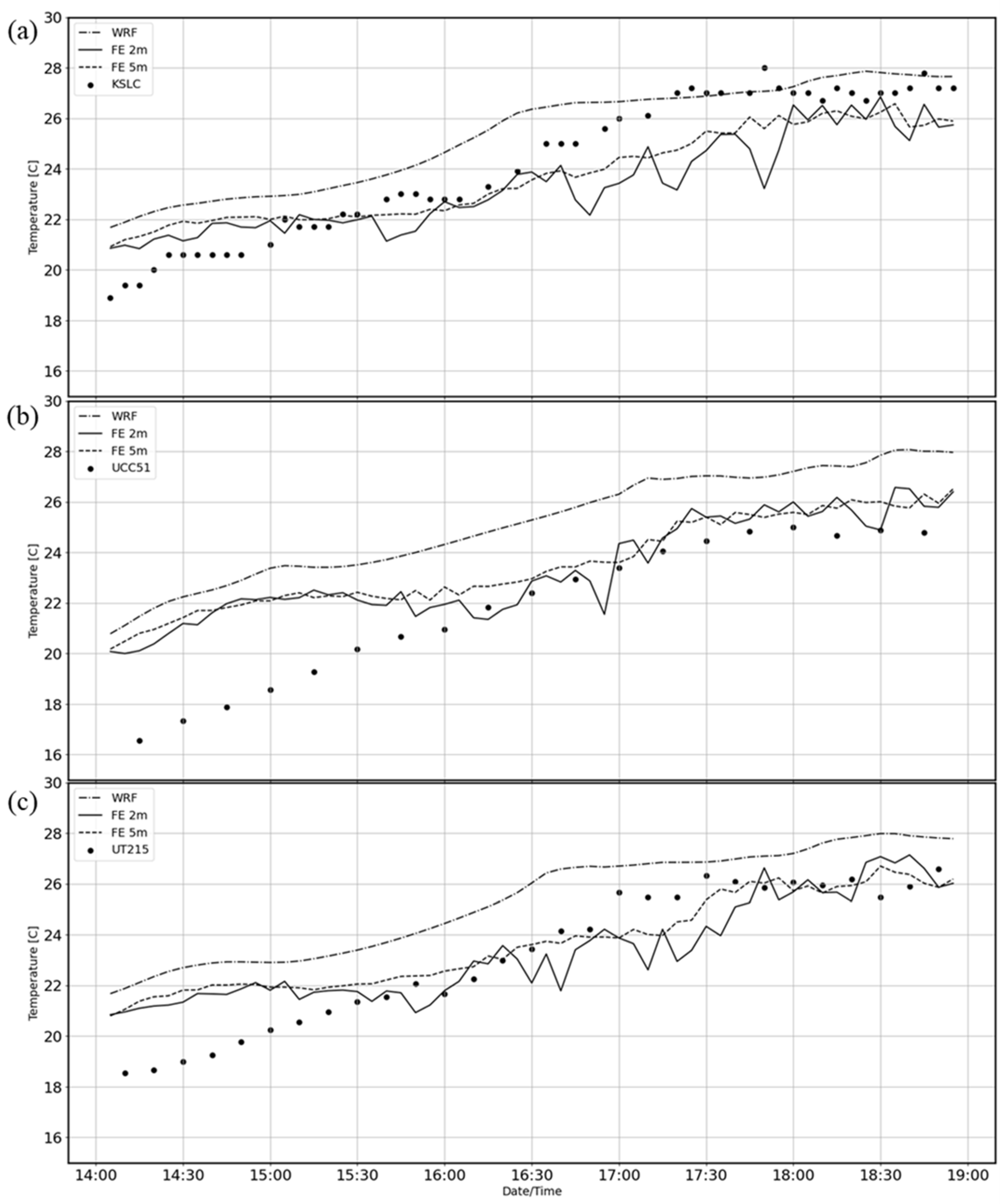
As shown in Figure 11a, the WRF 2 m temperatures are consistently higher than those observed at the SLC Airport (KSLC) in the initial hours of the simulation. The high observed temperatures after 17:30 UTC at this site are partly due to its location over a gravel surface surrounded by extensive concrete and pavement. Other observations within the FE domain remain lower than the WRF throughout the simulation (e.g., Figure 11b,c). UCC51 is located in a city park with extensive grass and trees. UT215 is located at the intersection of I-15 and I-215 near the airport. The FE 2 m temperatures are comparable to those observed after 15:00 UTC, while those at 5 m approach those simulated by WRF.
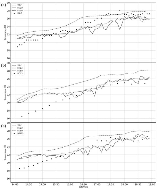
Figure 11.
Observed 2 m air temperature (°C, dots) between 14:00 and 19:00 UTC at: (a) KSLC; (b) UCC51; and (c) UT215. Also shown are time series of WRF air temperature and FE 2 m and 5 m air temperature at these locations by dash-dot, long dash and short dash lines, respectively.
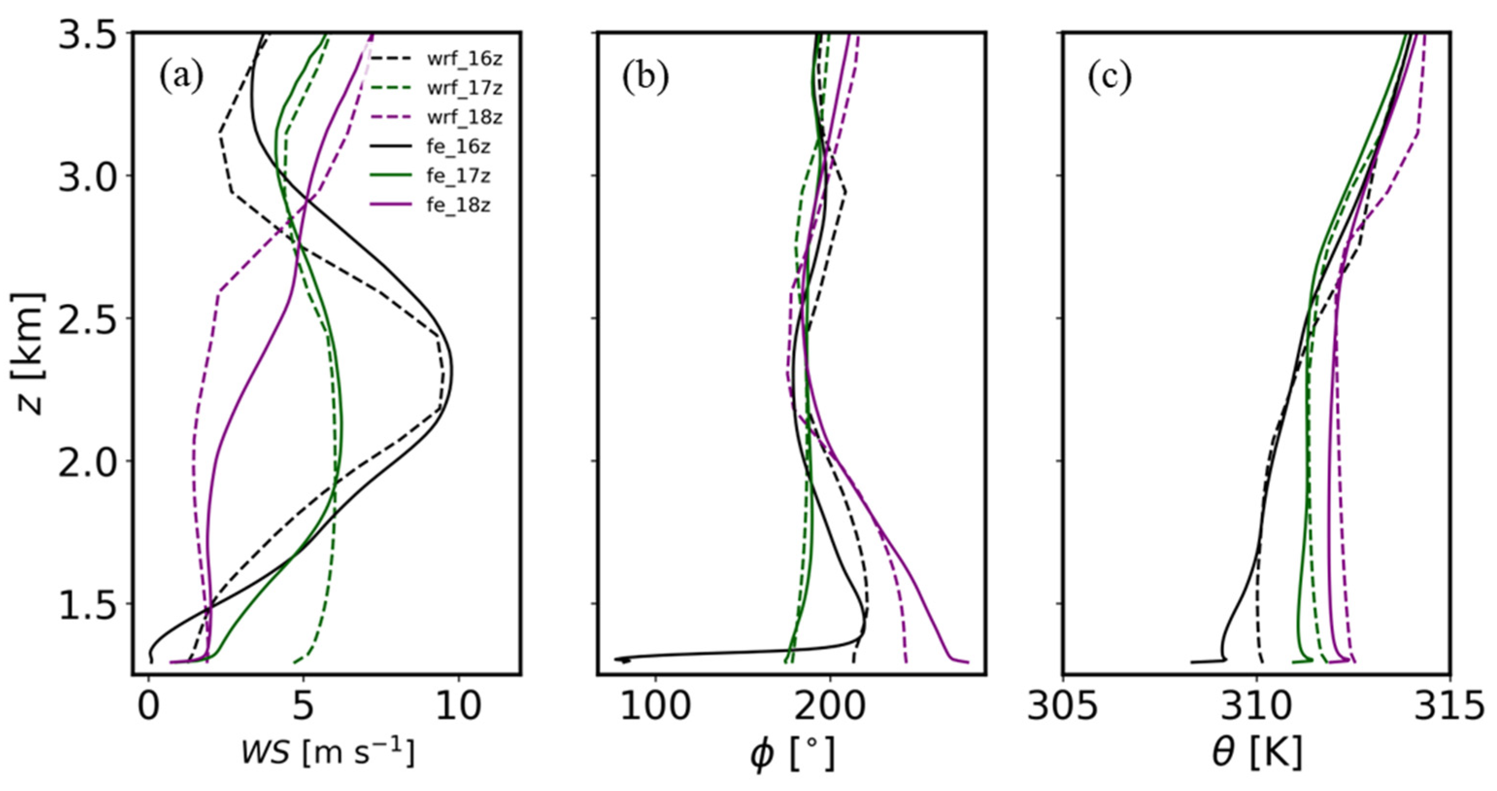
Figure 12 compares the vertical profiles of θ, wind speed, and wind direction averaged across non-building points within the 9 km × 9 km domain in both the WRF and FE simulations. While the FE and WRF southerly wind speeds aloft above 2 km MSL tend to be comparable, the FE domain-averaged near-surface winds are easterly and weaker relative to the WRF’s southerly winds. The WRF’s increase in southerly flow from 16:00 to 17:00 UTC near the ground is less evident in the FE simulation. Also, the faster progression of the front in the FE simulation, which aligned with TDWR observations, leads to more westerly winds by 18:00 UTC than simulated by WRF across the domain.
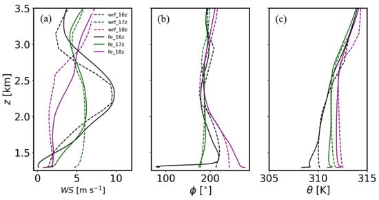
Figure 12.
As in Figure 4, except from the WRF (dashed) and FE (solid) simulations at 16:00 UTC (black), 17:00 UTC (green), and 18:00 UTC (purple), for (a) wind speed, (b) wind direction, and (c) potential temperature.
The θ vertical profiles in Figure 12c highlight the impact of surface heating in both the WRF and FE simulations. The WRF skin temperature averaged over the FE domain increases from 13 °C to 38 °C from 12:00 to 18:00 UTC, which leads to an 8 K increase in 2 m θ during the same period. (Pavement temperatures at UT215 near the Airport increased from 17 °C to 34 °C during this period.) As seen also in Figure 4c and Figure 8, the WRF’s initial stable vertical profile in the early morning becomes by 18:00 UTC adiabatic to nearly 3 km MSL. The domain-average FE profiles of θ evolve similarly to those evident from the WRF simulation, except that they have lower θ near the ground. A distinctive 0.5–1 °C increase in θ develops between the two lowest model layers (2–5 m AGL) in the FE simulation during all three time periods. Hence, given the very high skin temperatures, the model’s 2 m air temperature and θ are lower than expected. The thermal plumes evident in the cross-sections in Figure 9 punch through this thin artificial inversion.
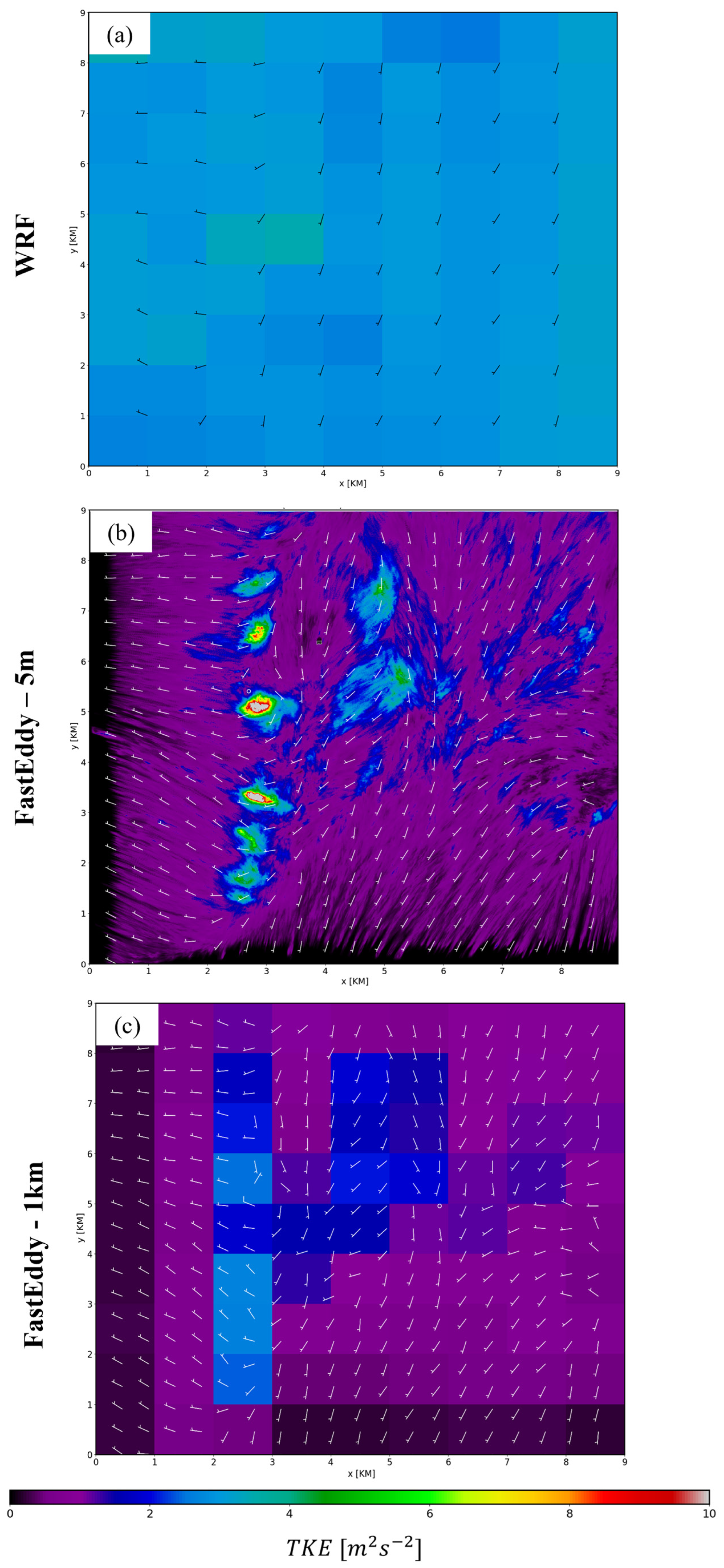
Comparing Figure 6 and Figure 7, there is a general tendency for 10 m AGL FE horizontal wind speeds to be lower than those simulated by WRF. The weaker wind field and the possible influence of the 2–5 m inversion layer may help to explain the lower production of TKE in the FE simulation compared to WRF (Figure 13). WRF TKE values of ~3–3.5 m2s⁻2 at 30 m AGL shown in Figure 13a represent the sub-1 km parameterized estimate of TKE over the 15 min period centered at 17:30 UTC. Figure 13b shows the sum of FE resolvable scale TKE (5 m–1 km scales) and FE sub-5 m parameterized TKE. FE has lower TKE than WRF over much of the domain, with large FE TKE limited primarily to the north–south-aligned frontal zone at this time. The very low TKE along the FE’s inflow boundaries reflects the spatial scales required to spin up the turbulence [44,45,46,47]. Upscaling the FE TKE to the same 1 km resolution of WRF (Figure 13c) reinforces the differences between TKE in FE and WRF. It should be noted that WRF exhibited higher surface temperatures relative to station observations (Figure 11), which could lead to increased buoyant thermal production and, consequently, higher TKE. Irrespective of the likely overall underestimate of TKE in this FE simulation, the very large TKE values along the front in excess of 10 m2 s⁻2 indicate the types of situations that would hamper UAS operations.

Figure 13.
TKE (m2 s−2, shaded) at 30 m AGL at 17:30 UTC: (a) WRF; (b) FE; and (c) FE upscaled to 1 km. Vector winds plotted as in earlier figures.
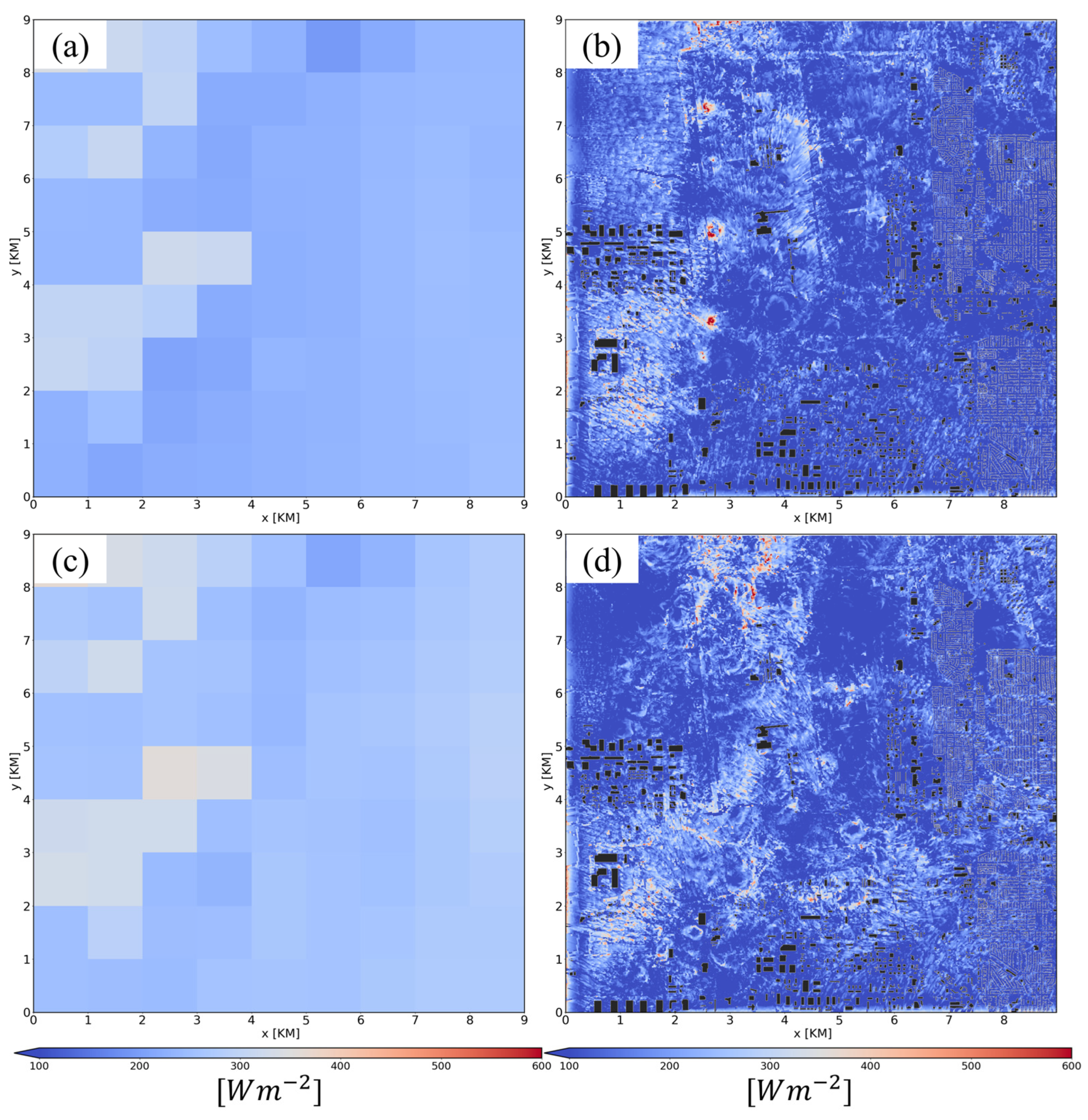
The potential causes for the FE’s inversion layer between 2 and 5 m and reduced TKE prompted us to consider the user-assigned thermal roughness parameter and its impacts on surface sensible heat flux. Late morning summer sensible heat fluxes in arid open [56] and urban areas [57] can be expected to be greater than 200 W m−2. The WRF heat flux at 17:30 and 18:00 UTC (Figure 14a and Figure 14c, respectively) typically exceeds that threshold, particularly in the areas with low roughness lengths in WRF. FE sensible heat flux is similarly higher (>300 W m−2) in the areas specified as having low roughness length (Figure 2d). The FE heat flux tends to be substantively lower in wetland regions (upper left of Figure 2b,d) but also unexpectedly low in urban areas with high roughness lengths (center left and right of Figure 2b,d). In addition, the sensible heat flux is zero where buildings are present. These characteristics have not been explicitly recognized previously as affecting other FE simulations since sensible heating has been less dominant than dynamical forcing during those simulations.
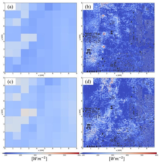
Figure 14.
Sensible heat flux (W m−2) shaded according to the colorbars: (a) WRF heat flux at 17:30 UTC; (b) as in (a) except for FE heat flux; (c) as in (a) except at 18:00 UTC; (d) as in (c) except for FE heat flux.
The sensible heat flux derived from the MOST-based FE surface layer parametrization scheme is affected by the treatment of surface roughness. The bulk transfer coefficients are computed using z0m from the NLCD reference list and user-prescribed z0h. These coefficients are then applied in the Noah land surface model bulk heat transfer equation to compute sensible heat flux. Given this setup, it is likely that the reduced heat flux was due to the weak user-prescribed z0h that induces negative feedbacks that tend to maintain lower near-surface temperatures, enhanced near-surface stability, and reduced near-surface wind speeds and TKE.
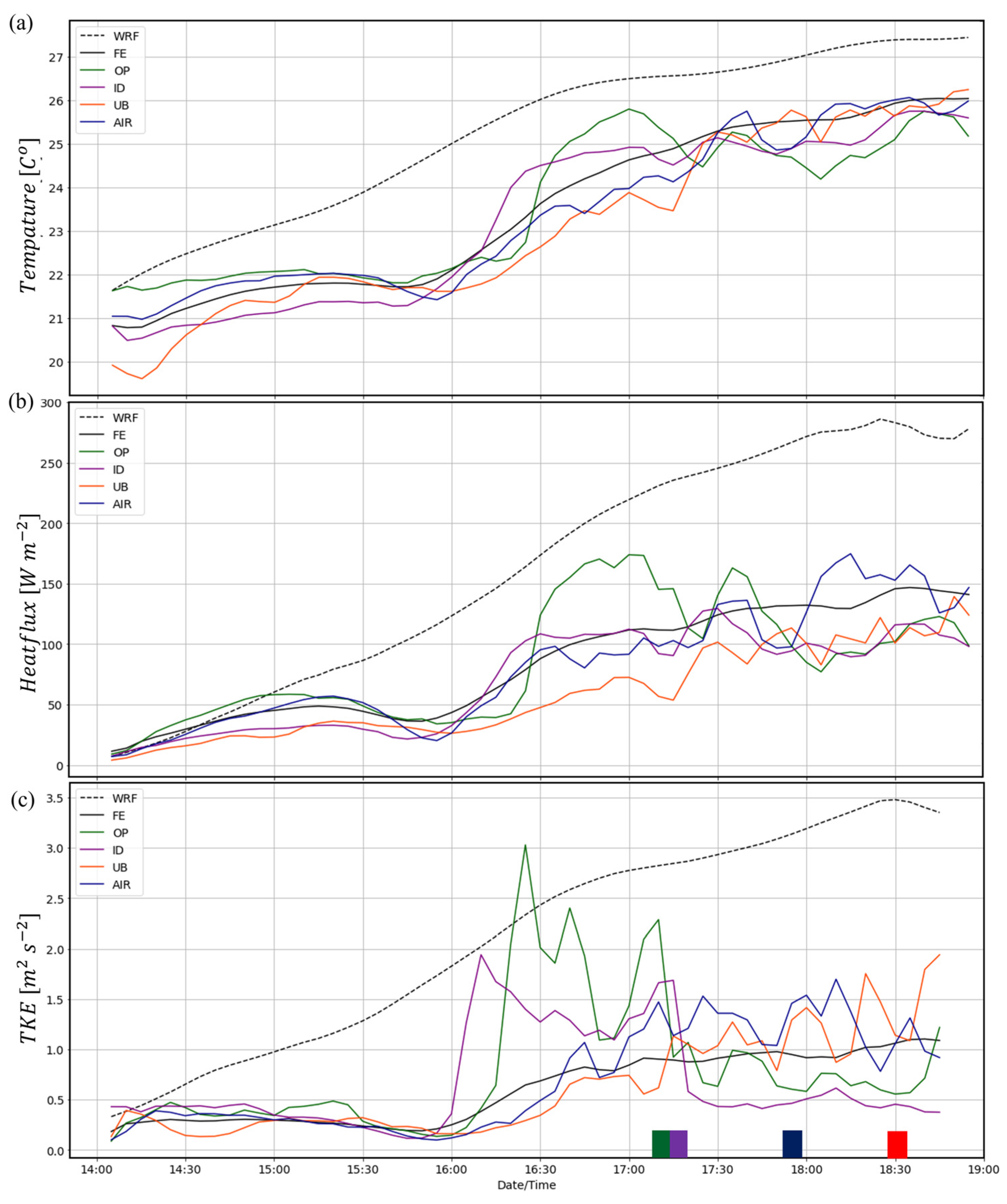
Figure 15 summarizes critical aspects of the FE simulation across the entire domain as well as in the subdomains shown in Figure 3. The 2 m air temperature (Figure 15a), heat flux (Figure 15b), and TKE (Figure 15c) remained relatively unchanged and lower than simulated by WRF between 14:00 and 16:00 UTC. As mentioned earlier, the underestimated specification of thermal roughness, z0h, reduces heat transfer efficiency and likely delays the destruction of the near-surface cold pool simulated during the morning. This reduction results in less sensible heat flux and provides insufficient energy to warm the near-surface air and increase turbulence during this period. After 16:00 UTC, lower FE 2 m air temperatures remain relative to WRF across the entire domain and within each subdomain (Figure 15a). As shown in Figure 15b, WRF sensible heat flux exceeds 200 W m−2 by 16:45 UTC (09:45 LST). Higher FE southerly wind speeds in advance of the lake breeze front at 16:30 UTC (Figure 7b) lead to sharp increases in air temperature, sensible heat flux, and TKE between 16:00 and 17:00 UTC in the Open (OP) and Industrial (ID) subdomains near the western edge of the FE domain (Figure 15). As indicated by the westerly wind shift in Figure 7c and increase in mixing ratio, the front crosses those areas by 17:30 UTC, after which the changes in temperature, sensible heat flux, and TKE tend to flatten (Figure 15). The temporary spikes in TKE, which were evident in these two areas between 17:15 and 17:30 UTC, resulted from the frontal passage. Since prefrontal southerly winds did not develop as strongly in the AP and UB subdomains (Figure 7), and the front weakens as it progresses further east (Figure 9), smaller peaks in sensible heat flux and TKE are present in those areas after 17:30 UTC.
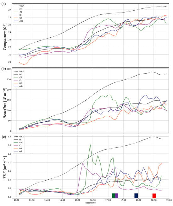
Figure 15.
Time series from 14:00 to 19:00 UTC: (a) 2 m air temperature (°C); (b) heat flux (W m−2); and (c) 30 m TKE (m2 s−2). Values are shown for domain-averaged WRF (dashed black line), domain-averaged FE (black line), and within the subdomains (OP, green; ID, purple; UB, red/orange; AP blue). The frontal passage in each subdomain (OP, ID, UB, AP) is indicated by the respective colored boxes along the x-axis.
4. Summary
This research uses the FE LES model to investigate the impact of an urban environment on boundary layer dynamics, temperature, wind, and turbulence. The GPU-based FE model is forced by one-way nested modeling simulations during which a lake breeze front traverses the SLC International Airport during the late morning LST on 3 June 2022. This study is the first application of FE to focus on boundary layer responses to strong surface heating and is configured to examine a GSL lake breeze frontal passage at a higher resolution than has been possible before. Using 64 GPUs (16 GPU nodes) on NCAR’s Derecho compute system, a 5 h FE simulation was completed in 18 h for an 81 km2 domain at Δ = 5 m horizontal resolution with 122 vertical levels. The level of resources required to complete such simulations is reasonable for sensitivity tests and for potentially developing improved microscale parameterizations relevant to other modeling systems.
The environment surrounding the SLC International Airport provides a rich mix of land surface and building types relevant to many other urban centers, including a nearby major water body, undeveloped wetlands, semi-arid fields, large commercial buildings, and neighborhoods encompassing homes and small commercial buildings. Our study is motivated by the need to examine the sensitivity of UAS flights to turbulence en route from distribution points near a major hub, such as the SLC Airport, to diverse locations within commercial and residential areas. Decisions to curtail flights when wind speeds exceed aircraft design thresholds are not likely to require fine-scale urban wind estimates from LES models such as FE. However, understanding how turbulence might affect flight operations, particularly on takeoff and landing, when the ambient mean wind is under such thresholds is not well understood. Much is being learned by flight reports from the ever-increasing number of UAS operations underway [17]. However, model simulations may help inform why many hazardous UAS flight situations develop and how to plan for them.
While this study presents results from only one FE simulation, many were completed as part of testing and evaluation in order for it to perform well in a relatively high elevation (~1230 m MSL), semi-arid environment. Intense surface heating transpires during a clear-sky, low-humidity summer morning. The skin temperature estimated from the WRF simulation increased from 13 to 38 °C during the morning, which appears reasonable relative to that observed on highway surfaces in the FE domain. In contrast, the GSL temperature during the morning likely only increased by 0.5 °C from the constant 19 °C specified in the WRF simulation based on remote sensing temperature estimates for that day, prior remote sensing studies (e.g., Crosman and Horel [58]), and unpublished 5 min buoy temperatures during earlier summers developed by the United States Geological Survey. This lake temperature is slightly lower than what is expected for 3 June 2022, which may have resulted in a more robust lake breeze front in the WRF simulation. The nocturnal and early morning down-valley winds observed through the Salt Lake Valley arise from mountain–valley and lake–land temperature differences that reverse to up-valley during late morning LST. The meteorological situation on 3 June 2022, with a well-defined lake breeze front traversing the FE domain in roughly one hour, is relatively common [30,33]. Observed station reports and TDWR radial wind speeds suggest that the FE simulation captures the general evolution underway during this period. However, the slower progression of the lake breeze front imposed by the WRF lateral boundary conditions on both the western and southern boundaries constrains details within the small FE domain. Several earlier FE studies examined mesoscale situations where strong external dynamical forcing was directed primarily in one direction such that the simulations were less affected by boundary forcing opposing the primary flow direction [24].
Lower TKE than expected during the FE simulation across much of the domain likely arose from underestimates of surface sensible heat flux, resulting from an assignment of thermal roughness lower than optimal. In this study, the user-prescribed FE surface thermal roughness length, z0h, was set to 10% of the surface roughness length, z0m. While this assumption appears appropriate in low roughness length areas within the FE domain, it leads to underestimates of the efficiency of heat transfer between the surface and the atmosphere and sensible heat flux in urban areas where z0m is higher. This reduced heat transfer leads to lower temperatures near the surface and enhances near-surface stability at the outset of the FE model simulation that is difficult to overcome since dynamical forcing then is weak. A later study will present additional simulations for this case in which increasing z0h leads to higher surface sensible heat flux.
In addition, the FE version used in this study does not consider direct radiative heating of buildings, which leads to substantial heating adjacent to the buildings [35,36,59]. Adding such building radiative effects would increase sensible heat fluxes wherever buildings are present.
Despite the underestimated TKE, the FE simulation captures turbulent interactions with the mean flow and buildings, highlighting physical processes that must be understood for UAS operations and air-quality studies [60,61]. Buoyant plumes develop in favored areas in response to the surface sensible heating that helps establish adiabatic mixing of momentum, heat, moisture, and pollutants with increasing depth as the morning progresses. Turbulent θ streaks illustrate the interaction between the ambient flow and structures, with wakes often evident in the lee of larger buildings. With over 20,000 buildings within the FE domain, the cumulative effect of these structures on the flow is, as expected, substantial.
The simulated structure of the lake breeze frontal head provides more detail than has been possible from observations [30,33] or WRF simulations at lower resolution [33]. Sharp horizontal gradients observed and simulated across the front and vertical velocities in excess of 3 m s−1 immediately in advance of it in the lowest km are capable of both increasing ozone concentrations at its leading edge and lofting them throughout the boundary layer [33]. As the simulated lake breeze front moves further away from the GSL, its depth and intensity weaken in a realistic fashion, partly due to the aforementioned imposed slower WRF frontal speed along the FE southern boundary.
A manuscript is being developed to assess the sensitivity of FE simulations for this case to removing all buildings, lowering the internal building temperature, and increasing the thermal surface roughness length so that the surface sensible heat flux is increased. In addition, work is underway to “fly” typical UAS package delivery drones along routes likely to be undertaken in the future using the turbulent wind fields available from the FE simulation in this study. The extent to which the drones would be affected by the turbulence along the flight path will be assessed.
Author Contributions
Conceptualization, B.M.W., J.D.H., and J.A.S.; methodology, B.M.W., J.D.H., and J.A.S.; software, J.A.S.; validation, B.M.W.; formal analysis, B.M.W.; investigation, B.M.W., J.D.H., and J.A.S.; computing resources, J.A.S.; writing—original draft preparation, B.M.W.; writing—review and editing, B.M.W., J.D.H., and J.A.S.; visualization, B.M.W. All authors have read and agreed to the published version of the manuscript.
Funding
This work was supported in part by the National Weather Service through the NOAA Collaborative Science, Technology, and Applied Research (CSTAR) Program Grant NA20NWS4680046 and the National Science Foundation Award 2330582. Sauer’s contributions to this work were unfunded.
Institutional Review Board Statement
Not applicable.
Informed Consent Statement
Not applicable.
Data Availability Statement
The NCAR Fasteddy® GPU model is open source [42] and the version used in this manuscript can be made available upon request to the following email: fasteddy@ucar.edu. The data presented in this study are available on request from the corresponding author due to the size of the data files. FastEddy is being actively developed at: https://github.com/NCAR/FastEddy-model (accessed on 10 January 2023). Lidar data (USGS LPC UT Wasatch L4 2013 LAS 2016) obtained from the United States Geological Survey archived on the OpenTopography webpage [48], and Salt Lake City building footprints obtained from Utah Geospatial Resource Center [49] were used in the creation of the three-dimensional buildings. Meteorological observations in the region used in this study were accessed through the Synoptic Data API services (https://synopticdata.com/mesonet-api [accessed on 8 August 2022]). Figures were made with Matplotlib version 3.4.3 [62,63], available under the Matplotlib license at https://matplotlib.org/ (accessed on 8 August 2022). Buildings used in the FastEddy simulation were generated in ArcGIS Pro version 3.2.1, available at https://www.esri.com/en-us/arcgis/products/arcgis-pro/overview (27 May 2021).
Acknowledgments
We would like to thank Aaron McCutchan for supplying the TDWR images and Amanda Siems-Anderson for her invaluable contributions. This research arose through the lead author’s participation in the NCAR ASP Graduate Visitor Program under the mentorship of Amanda Siems-Anderson and co-author Sauer. The University of Utah Center for High Performance Computing (CHPC) provided computational hardware and software necessary to analyze model simulations.
Conflicts of Interest
The authors declare no conflicts of interest.
References
- Pinto, J.O.; O’Sullivan, D.; Taylor, S.; Elston, J.; Baker, C.B.; Hotz, D.; Marshall, C.; Jacob, J.; Barfuss, K.; Piguet, B.; et al. The Status and Future of Small Uncrewed Aircraft Systems (UAS) in Operational Meteorology. Bull. Am. Meteorol. Soc. 2021, 102, E2121–E2136. [Google Scholar] [CrossRef]
- Klipp, C.L.; Measure, E. Urban Turbulence and Wind Gusts for Micro Air Vehicle Bio-Inspired Designs; Defense Technical Information Center: Fort Belvoir, VA, USA, 2011. [Google Scholar] [CrossRef]
- Glasheen, K.; Pinto, J.; Steiner, M.; Frew, E.W. Experimental Assessment of Local Weather Forecasts for Small Unmanned Aircraft Flight. In AIAA Scitech 2019 Forum; AIAA SciTech Forum; American Institute of Aeronautics and Astronautics: Reston, VA, USA, 2019. [Google Scholar] [CrossRef]
- Dudhia, J. A history of mesoscale model development. Asia-Pac. J. Atmos. Sci. 2014, 50, 121–131. [Google Scholar] [CrossRef]
- Benjamin, S.G.; Weygandt, S.S.; Brown, J.M.; Hu, M.; Alexander, C.R.; Smirnova, T.G.; Olson, J.B.; James, E.P.; Dowell, D.C.; Grell, G.A.; et al. A North American Hourly Assimilation and Model Forecast Cycle: The Rapid Refresh. Mon. Weather Rev. 2016, 144, 1669–1694. [Google Scholar] [CrossRef]
- Dowell, D.C.; Alexander, C.R.; James, E.P.; Weygandt, S.S.; Benjamin, S.G.; Manikin, G.S.; Blake, B.T.; Brown, J.M.; Olson, J.B.; Hu, M.; et al. The High-Resolution Rapid Refresh (HRRR): An Hourly Updating Convection-Allowing Forecast Model. Part I: Motivation and System Description. Weather Forecast. 2022, 37, 1371–1395. [Google Scholar] [CrossRef]
- Rai, R.K.; Berg, L.K.; Kosović, B.; Haupt, S.E.; Mirocha, J.D.; Ennis, B.L.; Draxl, C. Evaluation of the Impact of Horizontal Grid Spacing in Terra Incognita on Coupled Mesoscale–Microscale Simulations Using the WRF Framework. Mon. Weather Rev. 2019, 147, 1007–1027. [Google Scholar] [CrossRef]
- Wyngaard, J.C. Toward Numerical Modeling in the “Terra Incognita”. J. Atmos. Sci. 2004, 61, 1816–1826. [Google Scholar] [CrossRef]
- Chrit, M.; Majdi, M. Improving Wind Speed Forecasting for Urban Air Mobility Using Coupled Simulations. Adv. Meteorol. 2022, 2022, e2629432. [Google Scholar] [CrossRef]
- Honnert, R.; Efstathiou, G.A.; Beare, R.J.; Ito, J.; Lock, A.; Neggers, R.; Plant, R.S.; Shin, H.H.; Tomassini, L.; Zhou, B. The Atmospheric Boundary Layer and the “Gray Zone” of Turbulence: A Critical Review. J. Geophys. Res. Atmos. 2020, 125, e2019JD030317. [Google Scholar] [CrossRef]
- Kealy, J.C. Probing the ‘grey zone’ of NWP—Is higher resolution always better? Weather 2019, 74, 246–249. [Google Scholar] [CrossRef]
- Kochanski, A.K.; Pardyjak, E.R.; Stoll, R.; Gowardhan, A.; Brown, M.J.; Steenburgh, W.J. One-Way Coupling of the WRF–QUIC Urban Dispersion Modeling System. J. Appl. Meteorol. Climatol. 2015, 54, 2119–2139. [Google Scholar] [CrossRef]
- Li, Q.; Yang, J.; Yang, L. Impact of Urban Roughness Representation on Regional Hydrometeorology: An Idealized Study. J. Geophys. Res. Atmos. 2021, 126, e2020JD033812. [Google Scholar] [CrossRef]
- Ronda, R.J.; Steeneveld, G.J.; Heusinkveld, B.G.; Attema, J.J.; Holtslag, A. a. M. Urban Finescale Forecasting Reveals Weather Conditions with Unprecedented Detail. Bull. Am. Meteorol. Soc. 2017, 98, 2675–2688. [Google Scholar] [CrossRef]
- Singh, B.; Hansen, B.S.; Brown, M.J.; Pardyjak, E.R. Evaluation of the QUIC-URB fast response urban wind model for a cubical building array and wide building street canyon. Environ. Fluid Mech. 2008, 8, 281–312. [Google Scholar] [CrossRef]
- Wagenbrenner, N.S.; Forthofer, J.M.; Lamb, B.K.; Shannon, K.S.; Butler, B.W. Downscaling surface wind predictions from numerical weather prediction models in complex terrain with WindNinja. Atmos. Chem. Phys. 2016, 16, 5229–5241. [Google Scholar] [CrossRef]
- Pinto, J.O.; Jensen, A.A.; Jiménez, P.A.; Hertneky, T.; Muñoz-Esparza, D.; Dumont, A.; Steiner, M. Real-time WRF large-eddy simulations to support uncrewed aircraft system (UAS) flight planning and operations during 2018 LAPSE-RATE. Earth Syst. Sci. Data 2021, 13, 697–711. [Google Scholar] [CrossRef]
- Mi, L.; Han, Y.; Shen, L.; Cai, C.; Wu, T. Multi-Scale Numerical Assessments of Urban Wind Resource Using Coupled WRF-BEP and RANS Simulation: A Case Study. Atmosphere 2022, 13, 1753. [Google Scholar] [CrossRef]
- Roseman, C.A. Targeted Weather Forecasts for Small Unmanned Aircraft Systems; AMS: Perth, Australia, 2019. [Google Scholar]
- Wiersema, D.J.; Lundquist, K.A.; Mirocha, J.D.; Chow, F.K. Evaluation of Turbulence and Dispersion in Multiscale Atmospheric Simulations over Complex Urban Terrain during the Joint Urban 2003 Field Campaign. Mon. Weather Rev. 2022, 150, 3195–3209. [Google Scholar] [CrossRef]
- Sauer, J.A.; Muñoz-Esparza, D. The FastEddy® Resident-GPU Accelerated Large-Eddy Simulation Framework: Model Formulation, Dynamical-Core Validation and Performance Benchmarks. J. Adv. Model. Earth Syst. 2020, 12, e2020MS002100. [Google Scholar] [CrossRef]
- Muñoz-Esparza, D.; Sauer, J.A.; Jensen, A.A.; Xue, L.; Grabowski, W.W. The FastEddy® Resident-GPU Accelerated Large-Eddy Simulation Framework: Moist Dynamics Extension, Validation and Sensitivities of Modeling Non-Precipitating Shallow Cumulus Clouds. J. Adv. Model. Earth Syst. 2022, 14, e2021MS002904. [Google Scholar] [CrossRef]
- Muñoz-Esparza, D.; Sauer, J.A.; Shin, H.H.; Sharman, R.; Kosović, B.; Meech, S.; García-Sánchez, C.; Steiner, M.; Knievel, J.; Pinto, J.; et al. Inclusion of Building-Resolving Capabilities into the FastEddy® GPU-LES Model Using an Immersed Body Force Method. J. Adv. Model. Earth Syst. 2020, 12, e2020MS002141. [Google Scholar] [CrossRef]
- Muñoz-Esparza, D.; Shin, H.H.; Sauer, J.A.; Steiner, M.; Hawbecker, P.; Boehnert, J.; Pinto, J.O.; Kosović, B.; Sharman, R.D. Efficient Graphics Processing Unit Modeling of Street-Scale Weather Effects in Support of Aerial Operations in the Urban Environment. AGU Adv. 2021, 2, e2021AV000432. [Google Scholar] [CrossRef]
- Sagaut, P.; Lee, Y.-T. Large Eddy Simulation for Incompressible Flows: An Introduction. Scientific Computation Series. Appl. Mech. Rev. 2002, 55, 115. [Google Scholar] [CrossRef]
- Lilly, D.K. On the numerical simulation of buoyant convection. Tellus 1962, 14, 148–172. [Google Scholar] [CrossRef]
- Lilly, D.K. On the application of the eddy viscosity concept in the inertial sub-range of turbulence. NCAR Manuscript 1966, 123, 2–15. [Google Scholar]
- Ranquist, E. Exploring the Range of Weather Impacts on UAS Operations; AMS: Ann Arbor, MI, USA, 2017. [Google Scholar]
- Wang, B.H.; Wang, D.B.; Ali, Z.A.; Ting Ting, B.; Wang, H. An overview of various kinds of wind effects on unmanned aerial vehicle. Meas. Control. 2019, 52, 731–739. [Google Scholar] [CrossRef]
- Zumpfe, D.E.; Horel, J.D. Lake-Breeze Fronts in the Salt Lake Valley. J. Appl. Meteorol. Climatol. 2007, 46, 196–211. [Google Scholar] [CrossRef]
- Crosman, E.T.; Horel, J.D. Idealized Large-Eddy Simulations of Sea and Lake Breezes: Sensitivity to Lake Diameter, Heat Flux and Stability. Bound. -Layer Meteorol. 2012, 144, 309–328. [Google Scholar] [CrossRef]
- Crosman, E.T.; Horel, J.D. Large-eddy simulations of a Salt Lake Valley cold-air pool. Atmos. Res. 2017, 193, 10–25. [Google Scholar] [CrossRef]
- Blaylock, B.K.; Horel, J.D.; Crosman, E.T. Impact of Lake Breezes on Summer Ozone Concentrations in the Salt Lake Valley. J. Appl. Meteorol. Climatol. 2017, 56, 353–370. [Google Scholar] [CrossRef]
- Skamarock, C.; Klemp, B.; Dudhia, J.; Gill, O.; Liu, Z.; Berner, J.; Wang, W.; Powers, J.G.; Duda, M.G.; Barker, D.; et al. A Description of the Advanced Research WRF Model Version 4.1. Technical Note NCAR/TN-556+STR; The National Center for Atmospheric Research: Boulder, CO, USA, 2019. [Google Scholar] [CrossRef]
- Kusaka, H.; Kondo, H.; Kikegawa, Y.; Kimura, F. A Simple Single-Layer Urban Canopy Model for Atmospheric Models: Comparison with Multi-Layer and Slab Models. Bound. -Layer Meteorol. 2001, 101, 329–358. [Google Scholar] [CrossRef]
- Martilli, A.; Clappier, A.; Rotach, M.W. An Urban Surface Exchange Parameterisation for Mesoscale Models. Bound. -Layer Meteorol. 2002, 104, 261–304. [Google Scholar] [CrossRef]
- Chen, F.; Kusaka, H.; Bornstein, R.; Ching, J.; Grimmond, C.S.B.; Grossman-Clarke, S.; Loridan, T.; Manning, K.W.; Martilli, A.; Miao, S.; et al. The integrated WRF/urban modelling system: Development, evaluation, and applications to urban environmental problems. Int. J. Climatol. 2011, 31, 273–288. [Google Scholar] [CrossRef]
- Mughal, M.O.; Li, X.-X.; Norford, L.K. Urban heat island mitigation in Singapore: Evaluation using WRF/multilayer urban canopy model and local climate zones. Urban Clim. 2020, 34, 100714. [Google Scholar] [CrossRef]
- Salamanca, F.; Martilli, A.; Tewari, M.; Chen, F. A Study of the Urban Boundary Layer Using Different Urban Parameterizations and High-Resolution Urban Canopy Parameters with WRF. J. Appl. Meteorol. Climatol. 2011, 50, 1107–1128. [Google Scholar] [CrossRef]
- Sharma, A.; Fernando, H.; Hellmann, J.; Chen, F. Sensitivity of WRF Model to Urban Parameterizations, with Applications to Chicago Metropolitan Urban Heat Island; American Society of Mechanical Engineers, Fluids Engineering Division (Publication) FEDSM: Anaheim, CA, USA, 2014; Volume 1D. [Google Scholar] [CrossRef]
- Sharma, A.; Fernando, H.J.S.; Hamlet, A.F.; Hellmann, J.J.; Barlage, M.; Chen, F. Urban meteorological modeling using WRF: A sensitivity study. Int. J. Climatol. 2017, 37, 1885–1900. [Google Scholar] [CrossRef]
- Sauer, J.; Muñoz-Esparza, D.; Prestopnik, J. FastEddy-Model Software Release; NSF National Center for Atmospheric Research: Boulder, CO, USA, 2024. [Google Scholar] [CrossRef]
- Computational and Information Systems Laboratory. Derecho: HPE Cray EX System (University Community Computing); National Center for Atmospheric Research: Boulder, CO, USA, 2023. [Google Scholar] [CrossRef]
- Muñoz-Esparza, D.; Kosović, B.; Mirocha, J.; van Beeck, J. Bridging the Transition from Mesoscale to Microscale Turbulence in Numerical Weather Prediction Models. Bound. -Layer Meteorol. 2014, 153, 409–440. [Google Scholar] [CrossRef]
- Muñoz-Esparza, D.; Kosović, B.; van Beeck, J.; Mirocha, J. A stochastic perturbation method to generate inflow turbulence in large-eddy simulation models: Application to neutrally stratified atmospheric boundary layers. Phys. Fluids 2015, 27, 035102. [Google Scholar] [CrossRef]
- Muñoz-Esparza, D.; Lundquist, J.K.; Sauer, J.A.; Kosović, B.; Linn, R.R. Coupled Mesoscale-LES Modeling of a Diurnal Cycle during the CWEX-13 Field Campaign: From Weather to Boundary-Layer Eddies. J. Adv. Model. Earth Syst. 2017, 9, 1572–1594. [Google Scholar] [CrossRef]
- Mirocha, J.; Kirkil, G.; Bou-Zeid, E.; Chow, F.K.; Kosović, B. Transition and Equilibration of Neutral Atmospheric Boundary Layer Flow in One-Way Nested Large-Eddy Simulations Using the Weather Research and Forecasting Model. Mon. Weather Rev. 2013, 141, 918–940. [Google Scholar] [CrossRef]
- USGS 3DEP—USGS LPC UT Wasatch L4 2013 LAS 2016. Available online: https://portal.opentopography.org/usgsDataset?dsid=USGS_LPC_UT_Wasatch_L4_2013_LAS_2016 (accessed on 17 October 2023).
- UGRC—Utah Building Footprints. Available online: https://gis.utah.gov/products/sgid/location/building-footprints/ (accessed on 24 April 2024).
- Chan, S.T.; Leach, M.J. A Validation of FEM3MP with Joint Urban 2003 Data. J. Appl. Meteorol. Climatol. 2007, 46, 2127–2146. [Google Scholar] [CrossRef]
- Shin, H.H.; Muñoz-Esparza, D.; Sauer, J.A.; Steiner, M. Large-Eddy Simulations of Stability-Varying Atmospheric Boundary Layer Flow over Isolated Buildings. J. Atmos. Sci. 2021, 78, 1487–1501. [Google Scholar] [CrossRef]
- Mahrt, L. The bulk aerodynamic formulation over heterogeneous surfaces. Bound. -Layer Meteorol. 1996, 78, 87–119. [Google Scholar] [CrossRef]
- Chen, Y.; Yang, K.; Zhou, D.; Qin, J.; Guo, X. Improving the Noah Land Surface Model in Arid Regions with an Appropriate Parameterization of the Thermal Roughness Length. J. Hydrometeorol. 2010, 11, 995–1006. [Google Scholar] [CrossRef]
- Zheng, D.; Velde, R.; van der Su, Z.; Booij, M.J.; Hoekstra, A.Y.; Wen, J. Assessment of Roughness Length Schemes Implemented within the Noah Land Surface Model for High-Altitude Regions. J. Hydrometeorol. 2014, 15, 921–937. [Google Scholar] [CrossRef]
- Weston, M.; Chaouch, N.; Valappil, V.; Temimi, M.; Ek, M.; Zheng, W. Assessment of the Sensitivity to the Thermal Roughness Length in Noah and Noah-MP Land Surface Model Using WRF in an Arid Region. Pure Appl. Geophys. 2019, 176, 2121–2137. [Google Scholar] [CrossRef]
- Massey, J.D.; Steenburgh, W.J.; Hoch, S.W.; Jensen, D.D. Simulated and Observed Surface Energy Fluxes and Resulting Playa Breezes during the MATERHORN Field Campaigns. J. Appl. Meteorol. Climatol. 2017, 56, 915–935. [Google Scholar] [CrossRef]
- Rios, G.; Ramamurthy, P. A novel model to estimate sensible heat fluxes in urban areas using satellite-derived data. Remote Sens. Environ. 2022, 270, 112880. [Google Scholar] [CrossRef]
- Crosman, E.T.; Horel, J.D. MODIS-derived surface temperature of the Great Salt Lake. Remote Sens. Environ. 2009, 113, 73–81. [Google Scholar] [CrossRef]
- Boppana, V.B.L.; Xie, Z.-T.; Castro, I.P. Large-Eddy Simulation of Heat Transfer from a Single Cube Mounted on a Very Rough Wall. Bound. -Layer Meteorol. 2013, 147, 347–368. [Google Scholar] [CrossRef]
- Allwine, K.J.; Shinn, J.H.; Streit, G.E.; Clawson, K.L.; Brown, M. OVERVIEW OF URBAN 2000: A Multiscale Field Study of Dispersion through an Urban Environment. Bull. Am. Meteorol. Soc. 2002, 83, 521–536. [Google Scholar] [CrossRef]
- Horel, J.; Crosman, E.; Jacques, A.; Blaylock, B.; Arens, S.; Long, A.; Sohl, J.; Martin, R. Summer ozone concentrations in the vicinity of the Great Salt Lake. Atmos. Sci. Lett. 2016, 17, 480–486. [Google Scholar] [CrossRef]
- Caswell, T.A.; Droettboom, M.; Lee, A.; Sales De Andrade, E.; Hunter, J.; Hoffmann, T.; Firing, E.; Klymak, J.; Stansby, D.; Varoquaux, N.; et al. Matplotlib/Matplotlib: REL, Zenodo, v3.4.0. 2021; [Software]. [CrossRef]
- Hunter, J.D. Matplotlib: A 2D Graphics Environment. Comput. Sci. Eng. 2007, 9, 90–95. [Google Scholar] [CrossRef]
Disclaimer/Publisher’s Note: The statements, opinions and data contained in all publications are solely those of the individual author(s) and contributor(s) and not of MDPI and/or the editor(s). MDPI and/or the editor(s) disclaim responsibility for any injury to people or property resulting from any ideas, methods, instructions or products referred to in the content. |
© 2024 by the authors. Licensee MDPI, Basel, Switzerland. This article is an open access article distributed under the terms and conditions of the Creative Commons Attribution (CC BY) license (https://creativecommons.org/licenses/by/4.0/).

