Improvements and Extension of the Linear Carbon Sink Model

Abstract

While the simple model of the total atmospheric carbon sink effect as a linear function of concentration has provided excellent prediction results, several problems remained to be investigated and solved. The most obvious open issue is the correct treatment of land use change emissions. It turns out that the model improves by mostly neglecting these emissions after 1950. This effectively implies that land use change emissions have been constant and small since then. The key investigation starts with the observation that the total carbon sink has a short-term component that can be explained by temperature changes. The apparent paradox, why contrary to the short-term changes no temperature-caused trend can be detected, despite the fact that several contributing processes exhibit clear temperature dependency, is analyzed and explained. The result of this analysis leads to the model extension, where the total effect of absorptions and natural emissions are a linear function of concentration and temperature. This extended model not only explains current measurements but also paleo-climate data from ice core time series.

1. Introduction

When a complex system is analyzed, there are two possible approaches. The bottom-up approach investigates the individual components, studies their behaviour, creates models of these components, and puts them together in order to simulate the complex system. The top-down approach looks at the complex system as a whole and studies the way that the system responds to external signals, in the hope to find known patterns that allow conclusions to be drawn about the inner structure.

This paper aims at deepening the understanding of the relation between anthropogenic carbon emissions, ${\mathrm{CO}}_2$ concentration, and the carbon cycle by extending a previously constructed top-down model.

The relation between anthropogenic carbon emissions, ${\mathrm{CO}}_2$ concentration, and the carbon cycle has in the past mainly been investigated with the bottom-up approach. The focus of interest are carbon sinks, the processes that reduce the atmospheric ${\mathrm{CO}}_2$ concentration considerably below the level that would have been reached, if all ${\mathrm{CO}}_2$ remained in the atmosphere. There are three types of sinks that absorb ${\mathrm{CO}}_2$ from the atmosphere: physical oceanic absorption, the photosynthesis of land plants, and the photosynthesis of phytoplankton in the oceans. Although the mechanisms of carbon uptake are well understood in principle [1], there are model assumptions that cause divergent results.

The foundations of the best-known and widely used modelling concept, the Bern model, were laid by Oeschger and Wiesenthaler [2], where they use a box-diffusion model for the ocean carbon sink and a model for the land sink with plant growth and decay. They did not include phytoplankton in their model. Their carbon cycle model has been applied for predicting ${\mathrm{CO}}_2$ concentration as early as 1978 [3] and 1983 [4]. It has been integrated into a oceanic circulation model [5]. The concept has been further developed into what is now known as the Bern model [6], the technical details of which are described in the documentation of its public domain implementation [7]. The model is a four-box system based on impulse response functions with seven parameters. The box of the deep ocean is a diffusion model. The number and values of the parameters have changed in the past, up until 2013. Other authors, who are considered to be leading in the climate discussion, refer to the Bern model [8,9]. Due to the diffusion model of the deep ocean, the uptake potential for ${\mathrm{CO}}_2$ of the deep ocean is rather limited, implying that 20% of all anthropogenic emissions will remain in the atmosphere without being absorbed. Whether the transport into the deep ocean is really as restricted as the Bern model claims is a serious open question. Newer findings on ocean influx [10] and phytoplankton [11] suggest a less restrictive transport model. According to [12] the carbon concentration (DIC) of the mixed layer is between 1800 and 2300 $\mathsf{\mu }$mol/kg, on average 2050 $\mathsf{\mu }$mol/kg, and in the deep ocean there is a higher concentration of appr. 2350 $\mathsf{\mu }$mol/kg [13], combined with upwelling ocean currents. This raises serious doubts about a simple diffusion mechanism as a model for the deep ocean. Furthermore, the Bern model does not include dependence on temperature, as it is embedded in climate models where there is a predefined causal relation from ${\mathrm{CO}}_2$ concentration to temperature, but not in the other direction.

There are only few investigations of the carbon cycle taking a top-down approach. Prior to the preceding paper, where the linear carbon sink model was formulated [14], to my knowledge only three publications have applied the top-down approach. In [1] three key sink mechanisms are investigated in a formal way, explaining why these absorptions can be linearized in relation to atmospheric ${\mathrm{CO}}_2$ concentration, and the overall absorption coefficient is computed from measured concentration and emission time series. The publication [15] is not just a top-down approach, because all aspects of the carbon cycle are treated. Harde deviates from the other approaches by focussing more on the short residence time, which incorporates all emissions, rather than the adjustment time after anthropogenic emissions. But he includes temperature as one driving factor of natural emissions. Finally, ref. [16] derived the linear model intuitively from observations of concentration growth and anthropogenic emissions, and the dependency of the sink effect on temperature fluctuations are described and are attributed to El Ni$\tilde{\mathrm{n}}$o. Also, the effect of Pinatubo and other volcanoes is described as an absorption pulse distributed over a few years.

The top-down models are built upon the assumption that all sink effects, land photosynthesis as well as ocean sink and phytoplankton photosynthesis, are linearly dependent on ${\mathrm{CO}}_2$ concentration, with the consequence that the atmospheric carbon can be modelled by a single linear first-order system. The underlying assumption is only the linearity; the actual absorption rate is estimated from measured data of high quality. Apart from the fact that this linearity assumption leads to consistent results over a more than 70-year period, additionally, the underlying processes have been analyzed to justify from first principles that they can be linearized within the range of realistically expected parameter values [1,14].

Recently, two more publications applied the linear sink model in their work. One interesting study [17] relates atmospheric ${\mathrm{CO}}_2$ concentration to the pH value of the ocean surface, and applies the linear sink model to this ${\mathrm{CO}}_2$ proxy. The key result of the study is that no saturation of the sink effect can be found in the mixed ocean layer. In [18], the linear sink model is presented as a didactic tool to understand atmospheric ${\mathrm{CO}}_2$ concentration in relation to anthropogenic emissions.

The strength of the top-down approach is that it is guided by measurements and statistical analysis of measured data series, with up to now only two model parameters. The implicit necessary consequence of this simple model is, that the uptake capacity of the deep ocean is large enough and sufficiently turbulent that no saturation effect will be noticeable in the foreseeable future. A significant increase in the upper ocean concentration would reduce the sink effect. Therefore, in our previous paper we investigated whether any significant deviation from the strict linearity can be detected by means of statistical tests. Based on emission and concentration data of the last 70 years, not the slightest deviation from the linear relation between the total carbon sink effect and ${\mathrm{CO}}_2$ concentration could be detected [14].

With current knowledge and data, it cannot be finally decided yet which approach makes more reliable predictions for the future. We know that the Bern model makes rather pessimistic predictions about future ${\mathrm{CO}}_2$ concentration, so its estimation can be used as an upper limit, whereas the linear sink model may be considered as an optimistic lower limit.

The Need for Extending the Linear Carbon Sink Model

The purpose of this paper is to take a closer look at the linear sink model, derive some conclusions from it, relax a previous assumption, and gain a deeper understanding of the underlying physical mechanisms.

In the previous paper, we established a simple robust approach on how to relate anthropogenic emissions and atmospheric ${\mathrm{CO}}_2$ concentration from the constraints given by physics [14]: The conservation of mass, leading to the continuity equation of the atmospheric carbon concentration, and the linearity between the sink processes and concentration.

The third assumption of constant average natural emissions has been a pragmatic choice, which will be questioned in this article.

While the simple model of the total atmospheric carbon sink effect as a linear function of concentration has provided excellent prediction results, several problems remain to be investigated and solved.

The most obvious open issue is the correct treatment of land use change emssions. These are emissions caused by changes in the natural carbon cycle such as deforestation and urban growth. A comprehensive introduction into the meaning of this type of emissions is given in [19]. It turns out, however, that prediction results of the model improve by mostly neglecting emissions caused by land use change after 1959.

Furthermore, a deeper analysis implies that the total sink effect can be explained by short-term temperature changes commonly known as El Ni$\tilde{\mathrm{n}}$o [16]. Why a long-term trend caused by temperature cannot be detected, despite the fact that several contributing processes exhibit temperature dependency, is analyzed and explained. Consequently, the sink model is extended to take care the effects of concentration and temperature correctly.

Apart from explaining the short-term variability of the current ${\mathrm{CO}}_2$ concentration growth the carbon sink model extended by temperature dependence also explains the relation between temperature and ${\mathrm{CO}}_2$ concentration of the Vostok ice core data quite convincingly.

All data sets used in this publication are well-known and undisputed standard data series, all of them referenced in the data availability statement. The carbon emission data, including the land use change emissions, are from the Global Carbon Budget [20], the ${\mathrm{CO}}_2$ concentration data are from Maona Loa [21], and the temperature time series is the global yearly sea surface temperature data set HadSST4 [22]. The historic ice core data are referenced and described in the section where they are used.

2. The Components of the Carbon Cycle

For understanding the mechanism of the total sink effect, it is necessary to understand the components of the carbon cycle and their dependencies [23]. Apart from the anthropogenic emissions and the human-caused land use change emissions, the two main sink systems communicating with the atmosphere are the ocean and the terrestrial sink system, whereby the ocean can be regarded as two separate systems, the deep ocean sink and the marine biota sink [1,24]. The sink systems consist of both emissions and absorption processes in relation to the atmosphere.

The oceans have both an emission process, upwelling in the warm ocean, as well as an absorption process, downwelling in the cold ocean. Both processes are governed by Henry’s law [25], whereby ${\mathrm{CO}}_2$ transport between atmosphere and water depends linearly on temperature [26] and on the concentration difference of ${\mathrm{CO}}_2$ between atmosphere and the top ocean layer, the mixed layer. Henry’s law applies to the state of equilibrium. Whereas the system as a whole is not in equilibrium, the relevant subsystem mixed layer (top 75 m of ocean) and atmosphere can be regarded to be in a state of equilibrium due to the known small relaxation time of appr. 1–2 years (compared to the time ranges relevant for climate changes). Some authors (e.g., [1]) treat the mixed layer as an extension of the atmosphere.

The concentration of ${\mathrm{CO}}_2$ in the mixed layer follows the concentration of the atmosphere, but the carbon transport into the ocean shows no indication of saturation yet [17].

In the net primary production process via photosynthesis, land plants as well as marine biota extract carbon from the atmosphere or the mixed layer of the ocean, respectively. Photosynthesis depends on the ${\mathrm{CO}}_2$ concentration, given enough water and other required nutrients, but also on temperature [27].

The respiration and decay processes directly depend on the available material and on the time constants of decay. They may also depend on temperature. Respiration and decay processes return carbon from land plants to the atmosphere and partly to the soil. Soil decay also returns carbon to the atmosphere.

The linear model assumes that all natural changes of ${\mathrm{CO}}_2$ concentration, including both emissions and absorptions, depend linearly on the total atmospheric ${\mathrm{CO}}_2$ concentration or can be linearized without a significant error. It is not necessary to know any of the individual emission or absorption parameters, because in a linear model they are all added up into a single parameter, which is estimated from the measured data. The formal justification for the linearity assumption of the key processes can be found in [1].

3. The Original Linear Carbon Sink Model

This description is a simplified version of the model described in [14]. When $C_i$ is atmospheric ${\mathrm{CO}}_2$ concentration at the end of year i, the increase in ${\mathrm{CO}}_2$ in the atmosphere $G_i$ during year i is

$$G_i=C_i-C_{i-1}.$$

(1)

For setting up the equation for mass conservation of ${\mathrm{CO}}_2$ in the atmosphere, we split the total yearly emissions into anthropogenic emissions $E_i$ during year i, and all other, predominantly natural emissions $N_i$ during year i. With all absorptions $A_i$ during year i the balance due to mass conservation becomes

$$G_i=E_i+N_i-A_i.$$

(2)

This means that atmospheric concentration growth is the difference between all emissions and all absorptions. Obviously emissions, absorptions, and concentration must be measured with the same unit. The natural unit for evaluating mass conservation would be Pg, but atmospheric masses are usually measured as concentration, relative to the total mass of the atmosphere. For emissions and absorption their masses translate into potential concentration change. Therefore, ppm is used here consequently, where 1 ppm (parts per million) is equivalent to 2.12 PgC (Petagram Carbon). This conversion factor is also used by IPCC [28].

We put the measurable properties to the left side of the equation, leaving the unknowns on the right side:

$$E_i-G_i=A_i-N_i$$

(3)

For simplification, more unknown than known emissions caused by land use change [20] are included in the unknown natural emissions $N_i$. This way of treating land use change emissons differs from the previous paper, the reason for which is explained in the next section.

The difference between the unknown absorptions and the unknown natural emissions is defined as the the sink effect $S_i$ during year i:

$$\begin{array}{ccc}\hfill S_i& =& \hfill A_i-N_i\hfill \\ & =& \hfill E_i-G_i.\hfill \end{array}$$

While the absorption and natural emission components are unknowns, the sink effect is known from measurements of anthropogenic emissions and the concentration growth. $S_i$ is modelled linearly with a constant absorption coefficient $a^0$ expressing the proportionality of the absorptions $A_i$ to concentration $C_{i-1}$ and a constant $n^0$ representing the annual natural emissions

$$\begin{array}{ccc}\hfill {\widehat{S}}_i^0& =& \hfill a^0·C_{i-1}-n^0\hfill \end{array}$$

(4)

$$\begin{array}{ccc}& =& \hfill a^0·(C_{i-1}-C^0)\hfill \end{array}$$

(5)

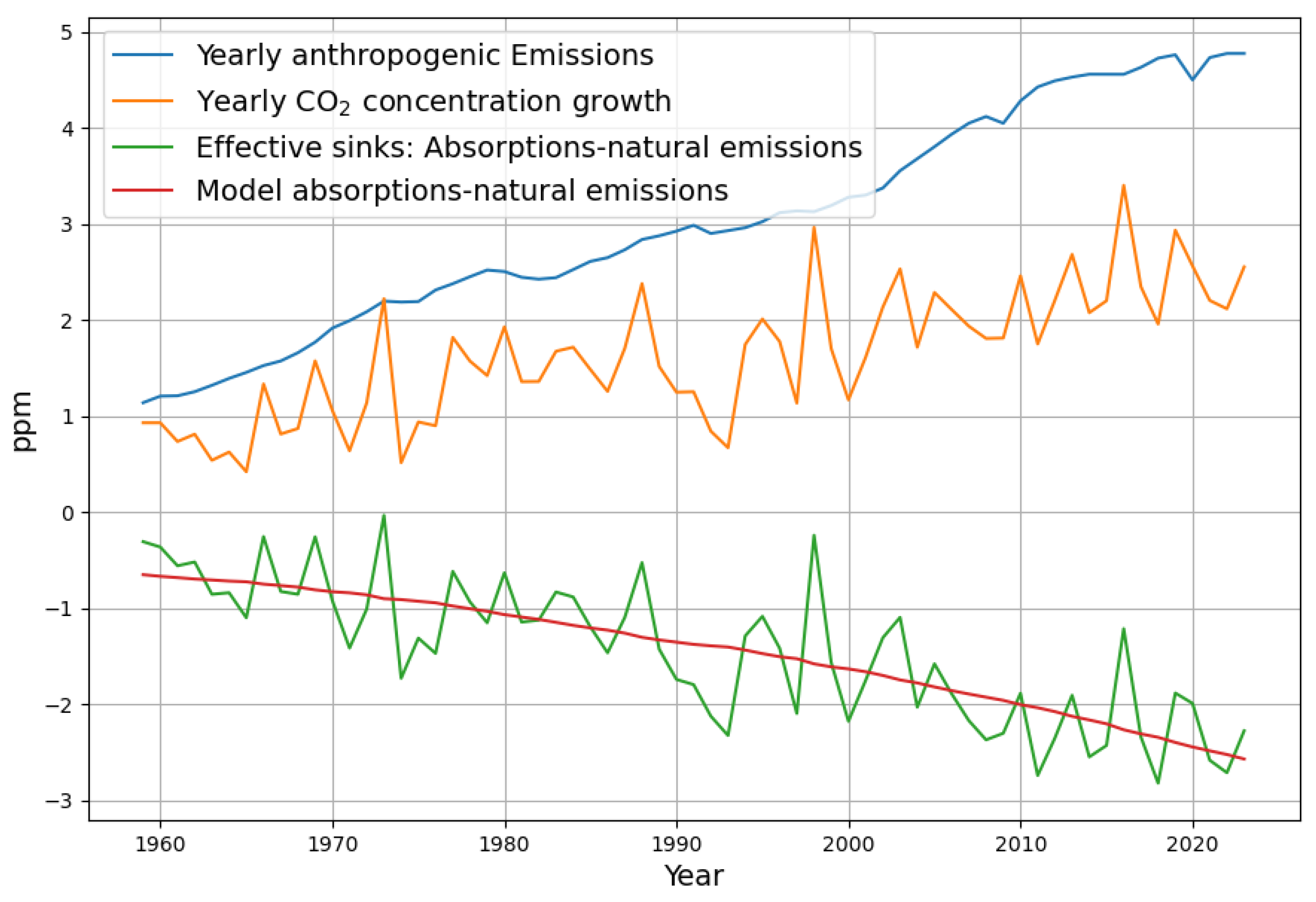
with $C^0=\frac{n^0}{a^0}$ as the equilibrium concentration which is eventually reached when anthropogenic emissions are zero. The estimated parameters of the least squares fit with annual data from 1959 to 2023 are $a^0=0.0183$, $n^0=5.2$ ppm, $C^0=284$ ppm. The time series of anthropogenic emissions, concentration growth, and the sink effect and its model are illustrated in Figure 1 (the sink effect and the sink model are drawn with a negative sign in order to keep the graphs visually separated).

When reconstructing or predicting modelled ${\mathrm{CO}}_2$ concentrations $\widehat{C_i}$, it is carried out by initiating

$${\widehat{C}}_{-1}=C_{-1}$$

where $C_{-1}$ is the measured concentration at the end of the year before the first year of the modelled time interval. The other items of the modelled concentration time series are determined by a recursion, derived from Equations (1), (3) and (4):

$${\widehat{C}}_i={\widehat{C}}_{i-1}+E_i-{\widehat{S}}_i^0$$

(6)

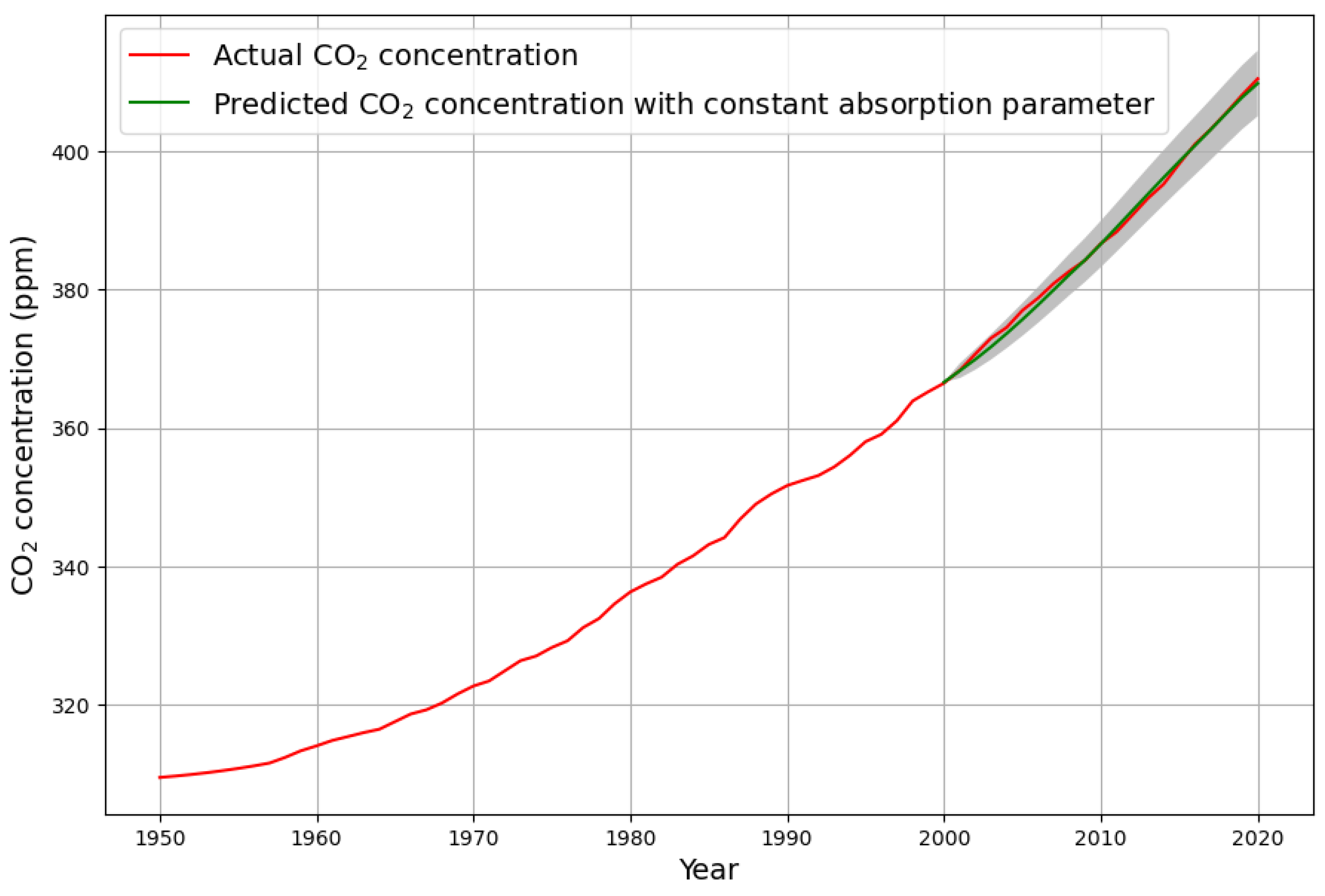
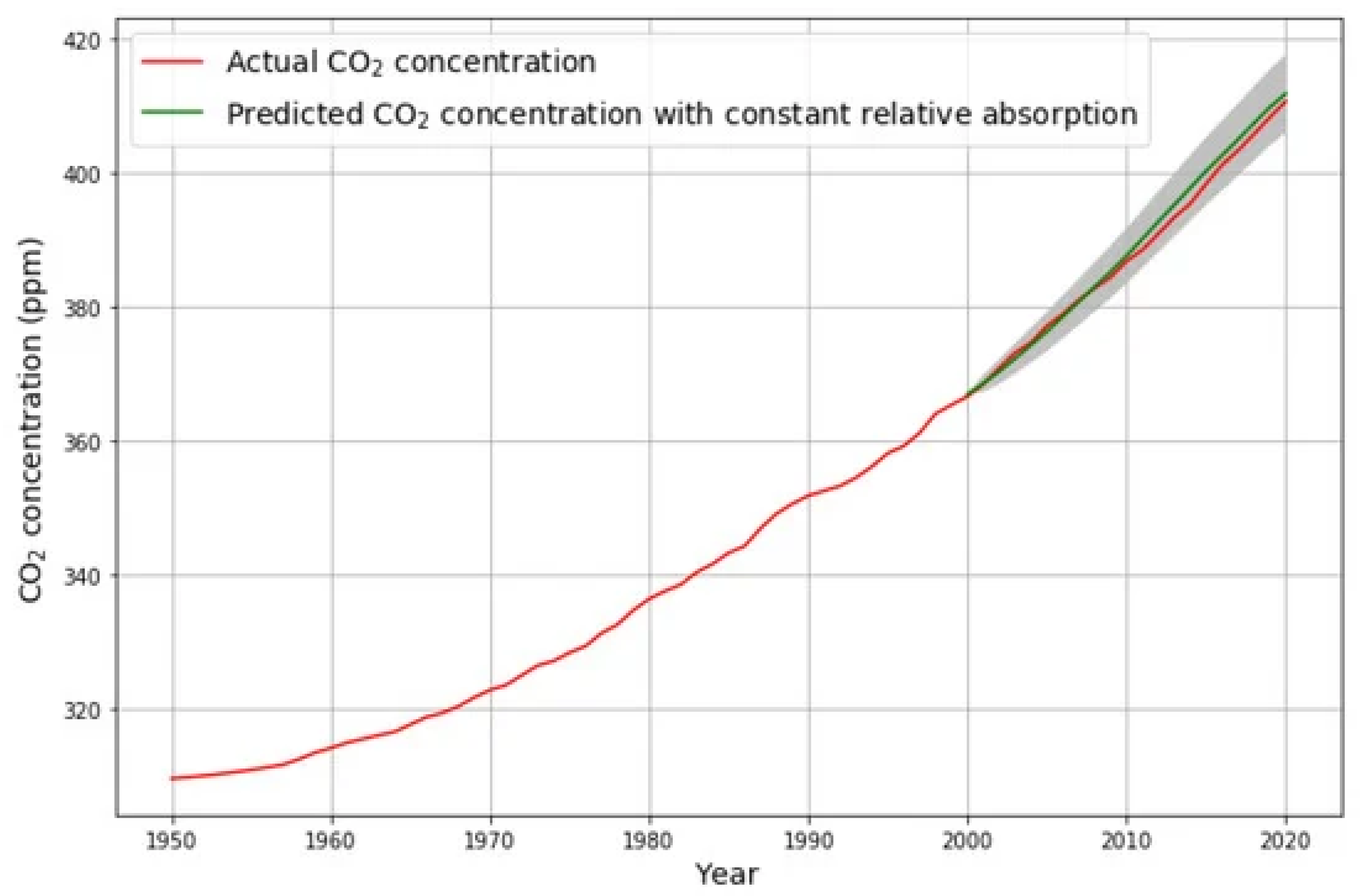
Figure 2 shows the comparison of the actual measured ${\mathrm{CO}}_2$ concentration with the predicted concentration data 2000–2020, using only data from 1950–1999 for the estimation of the model parameters. This shows the high quality of the prediction based on the linear model, using only data before the prediction time interval for estimating the model parameters. The 95% confidence interval of the prediction error, displayed as the grey shaded area, is extremely small.

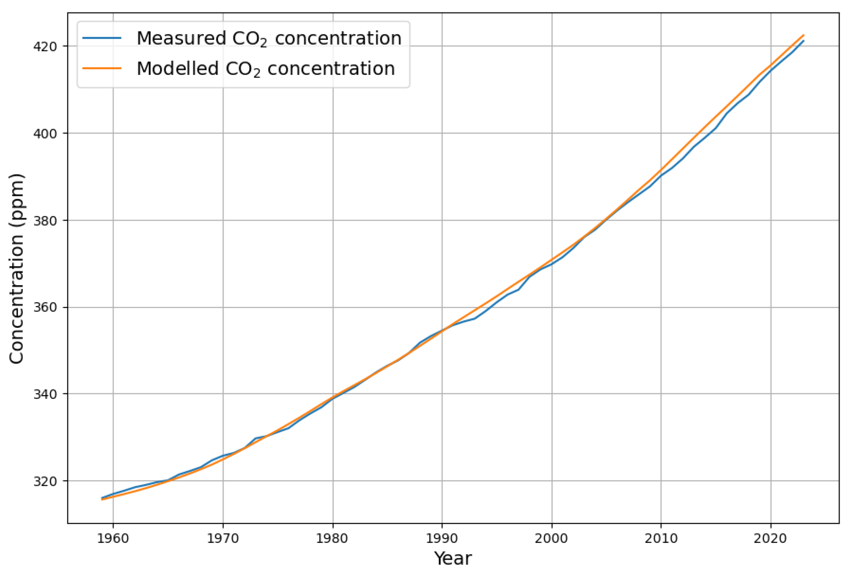
Another way of getting a sense for the quality of a model is to compare the model reconstruction with the original data within the range, from which the model was built. Figure 3 displays the comparison of the actual ${\mathrm{CO}}_2$ concentration data with their model reconstruction based on the linear model over the whole time range from 1959 to 2023. Attention is drawn to the deviation of the actual data from the model after 1990. This is one of the points that motivate the extension of the simple linear model. Surprisingly, the actual concentration is a bit smaller than the one predicted by the model. This suggests that no saturation of the sink effect is to be expected in the near future.

Identifying the Inflection Point in the ${\mathrm{CO}}_2$ Concentration

An important consequence of the linear sink model needs to be mentioned. When we look again at Figure 1, we clearly see that the large variability of the concentration growth is reflected in the sink effect. This variability is removed in the sink model, without changing the trend of the data. Therefore, the reconstructed concentration growth also does not exhibit its original short-term and random variability; its only “noise” is from the anthropogenic emission data.

From the recent publication of the CarbonBrief Project, we know that global emission data have been constant for more than 10 years [29]. From Equation (6), it follows that the estimated concentration growth is

$${\widehat{G}}_i=E_i-{\widehat{S}}_i^0$$

(7)

This means that with constant $E_i$ and a simultaneously increasing sink effect ${\widehat{S}}_i^0$ we expect declining concentration growth.

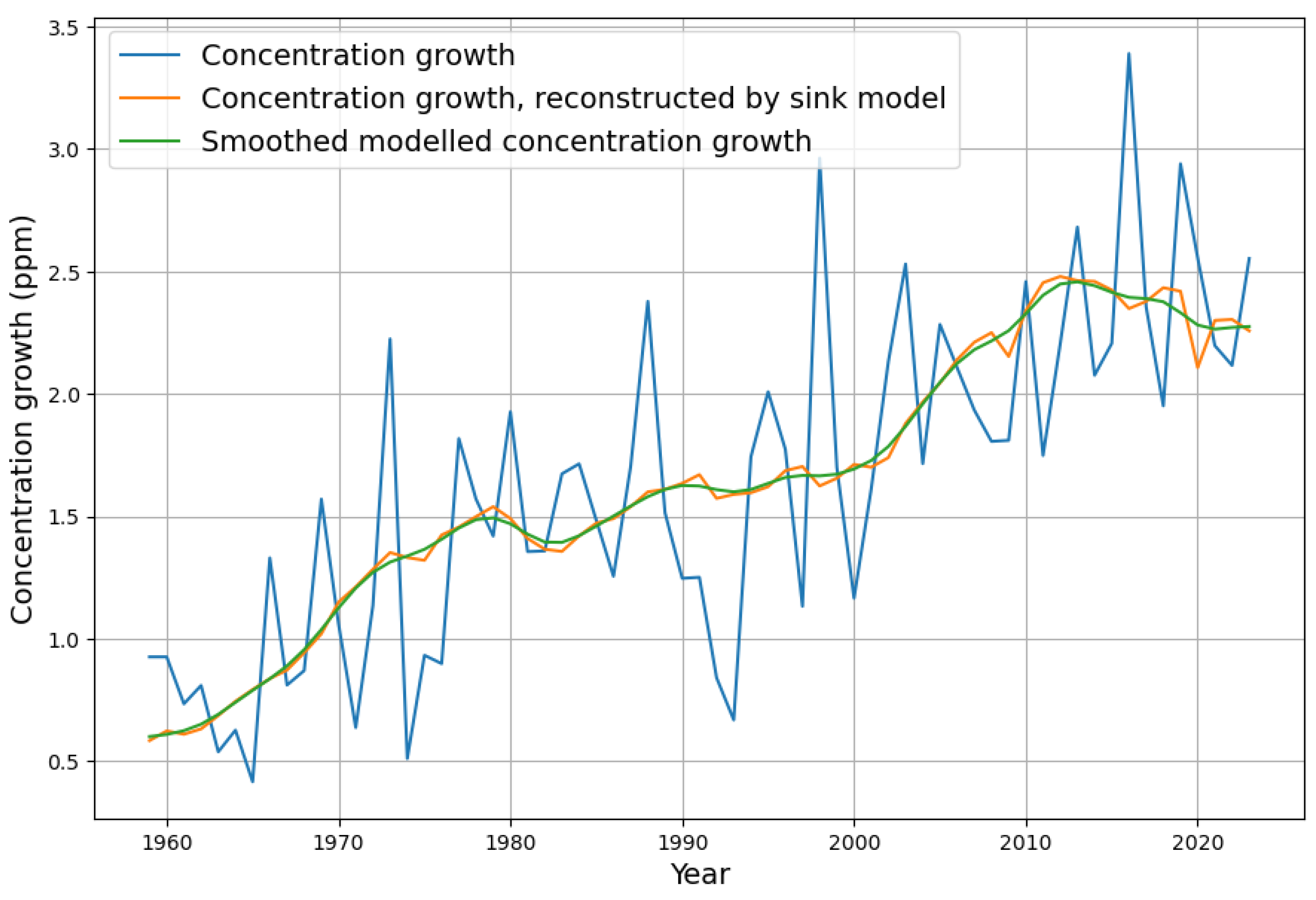
Figure 4 shows that the measured yearly concentration growth data have an absolute maximum in 2016 and a declining trend afterward. But the concentration growth data, when stripped of short-term and random effects, have their maximum already in 2013 and are declining since then. This means that the concentration graph has an inflection point in 2013, turning from concave to convex behaviour. The effect appears even clearer when emission data are also smoothed. This is a remarkable validation of a model prediction, and the fact that atmospheric carbon concentration growth is declining since 2013 has not been published before.

Figure 4 also explains why the significant drop in anthropogenic emissions in 2020 did not have any visible effect on concentration growth. The reconstructed “noise-free” concentration growth clearly shows the drop in emissions. But it so happens that this coincided with a positive spike in the “random” component of the concentration growth.

4. Making Land Use Change Emissions Consistent

When comparing the ex-post prediction in Figure 5 of 2000–2020 concentrations using the linear model with data from 1950–1999, where emissions caused by land use change were included (copied from [14]), with the new prediction in Figure 2 without explicit land use change emissions, it is obvious that the predictive quality has become considerably better when discarding explicit land use change emission data for estimating the model parameters.

This does not mean that there are no land use change emissions; it rather means that the best assumption is that they have been constant between 1950 and 2000 and beyond. It is a direct consequence of Equation (2) that constant annual land use change emissions ($LUC$) are interchangeable with natural emissions, so we can substitute the assumed “real” natural emissions $N_i^{\prime }$ and constant land use change emissions $LUC$ for $N_i$:

$$N_i=N_i^{\prime }+LUC$$

(8)

The most likely annual value of the land use change emissions during this specific time interval can be inferred from the assumption about the equilibrium ${\mathrm{CO}}_2$ concentration by postulating an equilibrium concentration value without land use change emissions, and let land use change account for the difference. This obviously assumes that the ocean and land sink mechanisms have remained rather stable over the time of observation.

We assume that the “real” equilibrium ${\mathrm{CO}}_2$ concentration value should be the same as the preindustrial assumed value of 280 ppm. Our estimate of the equilibrium based on anthropogenic emissions is $C^0=284$ ppm; therefore, from Equation (5) we can infer that between 1950 and 2020 the most likely annual value of the $LUC$ is

$$LUC=(284\mathrm{ppm}-280\mathrm{ppm})·a^0=4\mathrm{ppm}\times 0.0183=0.07\times 2.12\mathrm{PgC}=0.15\mathrm{PgC}$$

(9)

The measured data constrain the possible range of the land use change emissions. Increasing their assumed value implies lowering the equilibrium ${\mathrm{CO}}_2$ concentration. With the most likely equilibrium concentration of 280 ppm the best estimate for land use change emissions, they are a constant 0.15 PgC per annum.

This claim of land use change emissions contradicts the state-of-the-art findings in [20]. We see, however, no other possibility to reconcile the four constraints of anthropogenic emission measurements, concentration growth measurements, consistent sink coefficient, and equilibrium concentration consistent with preindustrial value of 280 ppm. The consistency of these constraints is reflected in the quality of prediction, as shown with the ex-post prediction of the 2000–2020 concentration data in Figure 2.

5. Extension of the Linear Sink Model

While the proportionality between absorption and concentration by means of an absorption constant $a^0$ is physically very well founded, the assumption of constant natural emissions appears arbitrary. Effectively, this assumed constant contains the sum of all emissions except the explicit anthropogenic ones and also all sinks that are balanced during the year. Therefore, it is enlightening to calculate the estimated natural emissions $\widehat{N_i}$ from the measured data and the mass balance equation with the estimated absorptison constant $a^0=0.0183$, see Equations (3) and (4):

$$\widehat{N_i}=G_i-E_i+a^0·C_{i-1}$$

(10)

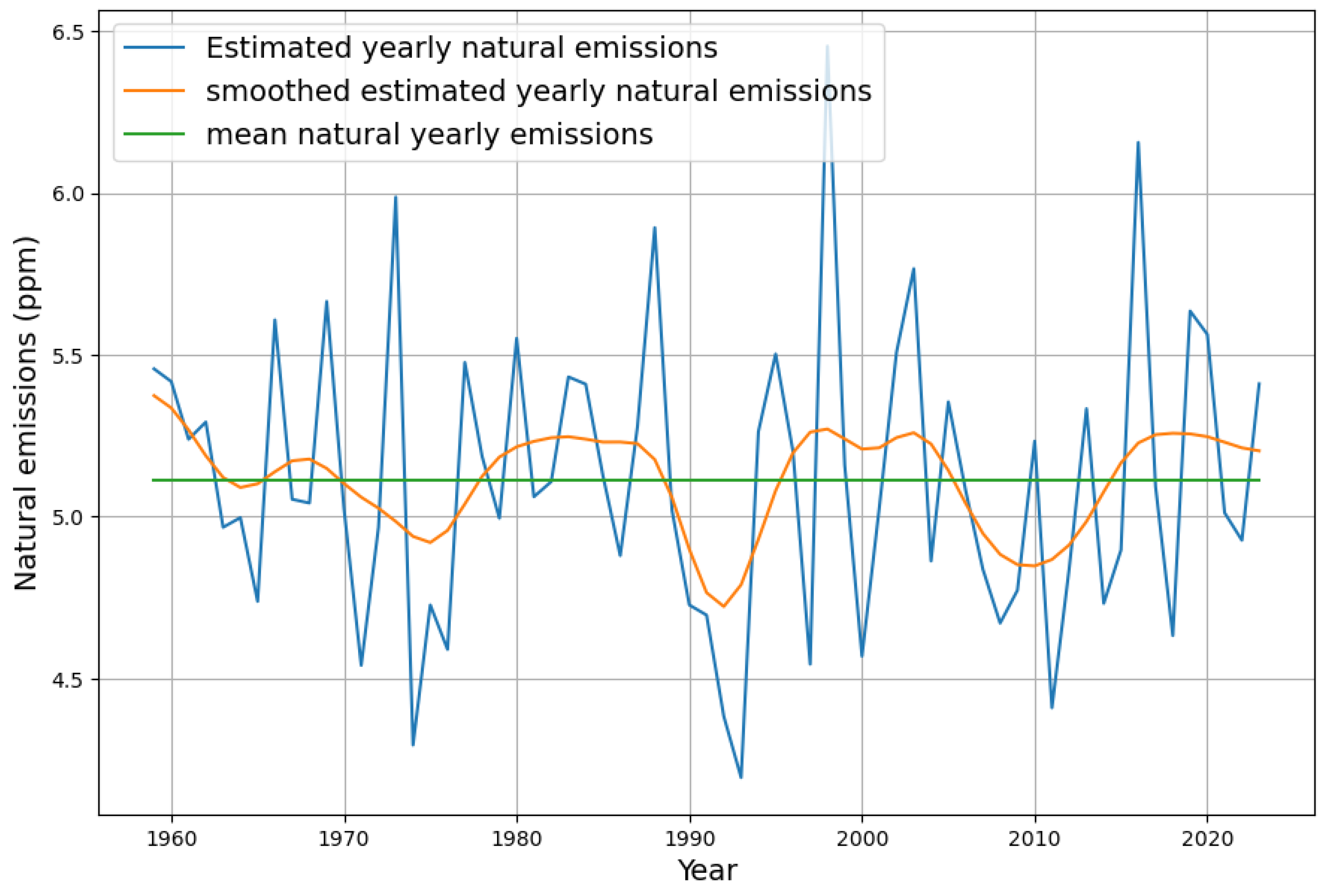
This is shown in Figure 6. The mean value of $\widehat{N_i}$ results in the constant model term $n^0$. Slight smoothing results in a periodic curve. Roy Spencer has attributed these fluctuations to El Ni$\tilde{\mathrm{n}}$o [16]. Questions arise: why and how are sources or sinks dependent on El Ni$\tilde{\mathrm{n}}$o? Why are short-term temperature dependencies present, but long-term global temperature trends do not appear to have any correspondence in the model? Furthermore, it is not obvious whether the fluctuations are attributable to the absorptions $A_i$ or to the natural emissions $N_i$. In order to find out more, we introduce a linear temperature dependence into the model.

The sink model is extended by a temperature term $T_i$, and the sign of the constant c is changed compared with the previous $n^0$:

$$\widehat{S_i}=a·C_{i-1}+b·T_i+c$$

(11)

These three regression parameters could be estimated directly, but in order to understand how the resulting numbers relate to the calculation without temperature dependence, we will motivate and build this model extension in an intuitive way.

5.1. ${CO}_2$ Concentration Is a Proxy for Temperature

Why can the undeniable long term temperature trend not be seen in the simple linear model? Why is there no trend in the estimated natural emissions? The answer has to do with the fact that ${\mathrm{CO}}_2$ concentration and temperature are highly correlated.

Therefore, any long term trend dependent on temperature would be attributed to ${\mathrm{CO}}_2$ concentration in a model based on concentration. Usually, in order to estimate the greenhouse effect, the relation between yearly average temperature $T_i$ and $log$ of yearly average ${\mathrm{CO}}_2$ concentration $log\left(C_i\right)$ is determined, but here we are interested in the linear relation between $T_i$ and $C_i$.

As a result, an approximation ${\widehat{T}}_i$ of the temperature anomaly can be derived from the concentration using a least squares fit of the linear function

$${\widehat{T}}_i=d·C_{i-1}+e$$

(12)

with $d=0.0083$°/ppm, $e=-2.72$°. Furthermore, the residual temperature $T_i^R$ is defined as

$$T_i^R=T_i-{\widehat{T}}_i$$

(13)

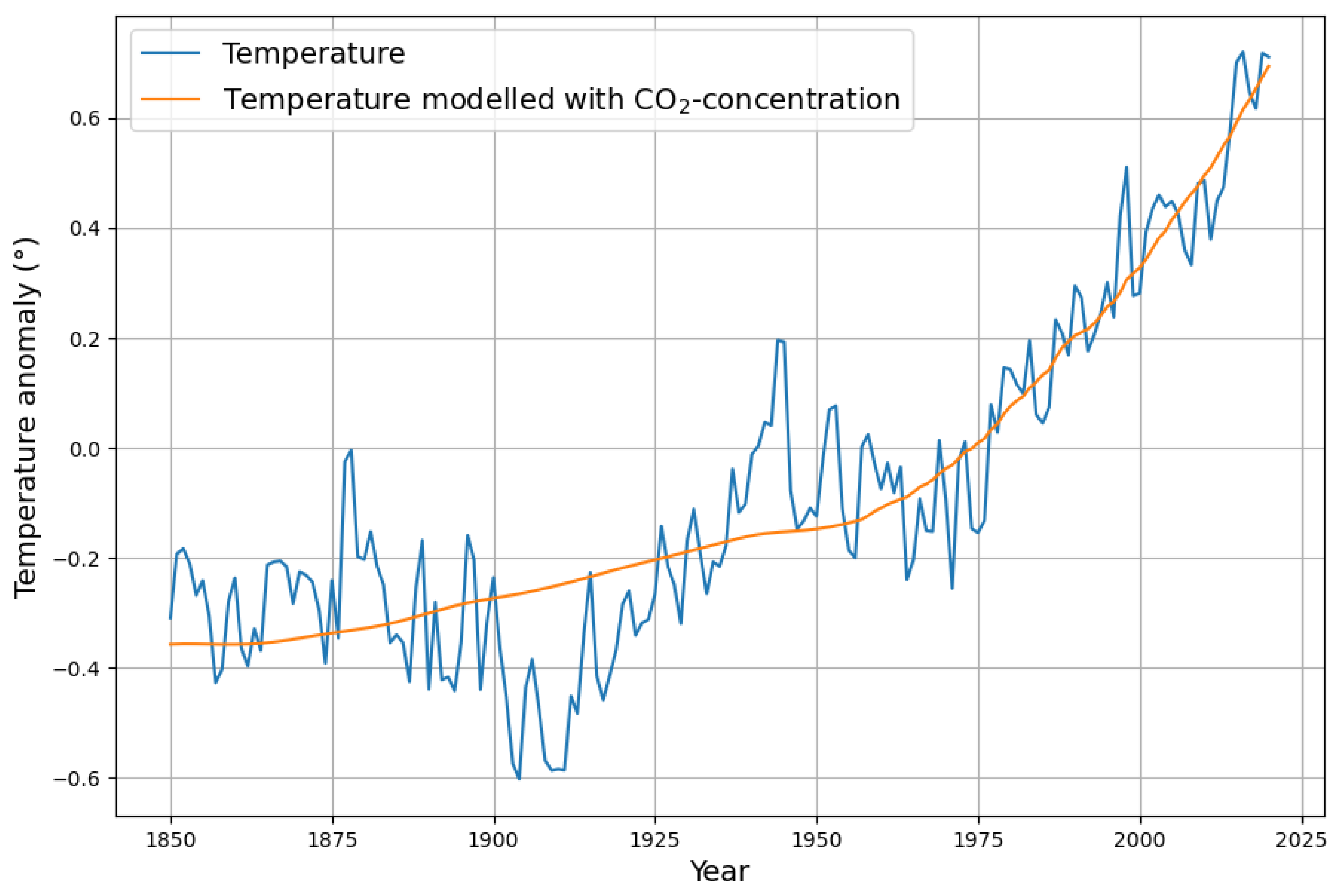
We make no claim of causality nor any other dependence between ${\mathrm{CO}}_2$ concentration and temperature, in either direction, but just recognize their strong correlation for the last 70 years. The optimal linear ${\mathrm{CO}}_2$ modelling for temperature anomaly based on the HadSST4 temperature data [22] is displayed in Figure 7.

5.2. Consequences of the ${CO}_2$ Temperature Proxy

The actual temperature $T_i$ is the sum of the modelled Temperature ${\widehat{T}}_i$ and the residual Temperature $T_i^R$. Therefore, the model equation becomes

$${\widehat{S}}_i=a·C_{i-1}+b·({\widehat{T}}_i+T_i^R)+c$$

(14)

Replacing ${\widehat{T}}_i$ with its ${\mathrm{CO}}_2$-concentration proxy

$${\widehat{S}}_i=a·C_{i-1}+b·(d·C_{i-1}+e+T_i^R)+c$$

(15)

and re-arrangement leads to

$${\widehat{S}}_i=(a+b·d)·C_{i-1}+b·T_i^R+(c+b·e).$$

(16)

Now, the temperature dependent part of the model depends by definition only on the residual zero mean variations of $T_i^R$, i.e., without any trend. All temperature trend information is covered by the coefficients of $C_i$. This model corresponds to Roy Spencer’s observation that much of the short-term variability is explained by El Ni$\tilde{\mathrm{n}}$o [16], which is closely related to the residual temperature $T_i^R$.

With $b=0$ we would have the temperature independent model, and the coefficients of $C_i$ and the constant term correspond to the known estimated parameters of the simple linear model. Due to the fact that $T_i^R$ does not contain any trend, the inclusion of this particular temperature-dependent term does not change the coefficients $a^0$ and $-n^0$.

The estimated parameters of the last equation are (in order to not confuse anomalies with actual standardized temperature, the anomaly measurement unit is written here as $°$ instead of $°$C)

$$\begin{array}{ccc}\hfill a+b·d& =& 0.0183=a^0\hfill \\ \hfill b& =& -2.9\mathrm{ppm}{/}^{\circ }\hfill \\ \hfill c+b·e& =& -5.2\mathrm{ppm}=-n^0.\hfill \end{array}$$

The first and last parameter correspond to those of the temperature-independent model. But now, from the estimated b coefficient, we can evaluate the contribution of temperature $T_i$ to the sinks and the natural emissions. The final model parameters are

$$\begin{array}{ccc}\hfill a& =& a_0-b·d=0.0436\hfill \\ \hfill b& =& -2.9\mathrm{ppm}{/}^{\circ }\hfill \\ \hfill c& =& -n^0-b·e=-13.6\mathrm{ppm}\hfill \end{array}$$

This means that the concentration-related assumed “true” annual absorption rate of 4.36% is much more than the 1.83% of the simple linear model. This higher absorption is compensated by temperature-dependent emissions, the annual base level of which (13.6 ppm) is also much larger than the 5.2 ppm of the simple linear model. Therefore this extended model reflects both the downwelling absorption in cold oceans as well as the upwelling emission in the warm oceans. An important question is whether we have any indication that this rather high absorption rate can be justified by measurements. Due to the nuclear bomb tests in the 1950s, which stopped in 1963, we have a close-to-ideal identifiable carbon emission pulse that has been thoroughly investigated for more than 40 years [30]. The resulting decreasing atmospheric${ }^{14}C$-concentration shows, over a 30-year time period, that the contributing absorption sink processes exhibit an undistorted exponential decay of a first order linear differential equation. The decay time of the resulting concentration curve has been determined to be 15 years [31], implying a yearly downwelling rate of $1/15\approx 6.7\%$. Although a small part (<$0.5\%/a$) of the${ }^{14}C$ concentration reduction in the atmosphere is due to the dilution effect of concentration increase through anthropogenic emissions [32], this indeed confirms that a yearly absorption rate of 4.36% is within a realistic range.

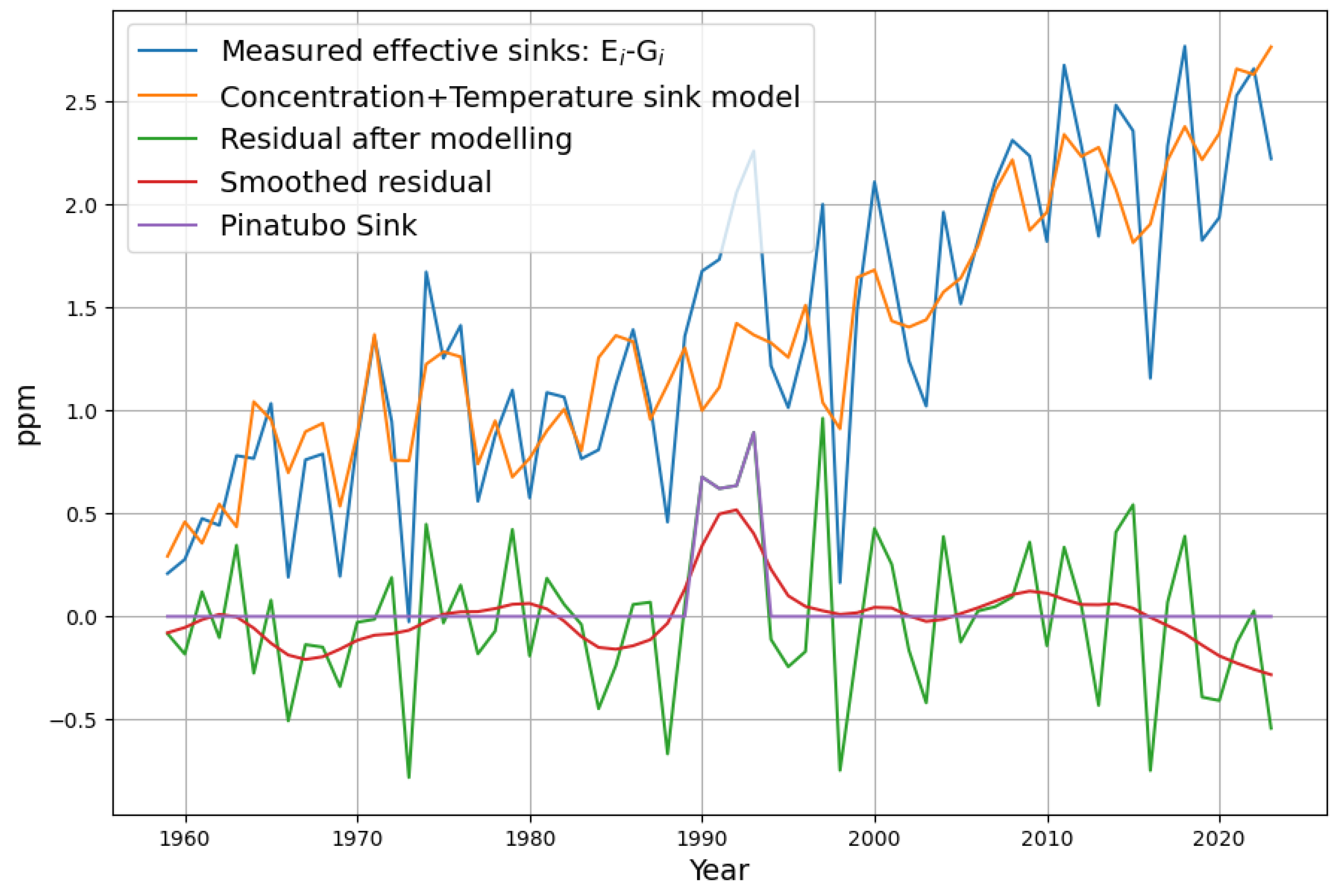
Figure 8 shows how closely the variations of temperature match the variations of the measured sinks.

The model reconstruction of the concentration is now using a sink term containing temperature as well as concentration:

$$\begin{array}{ccc}\hfill {\widehat{C}}_{-1}& =& \hfill C_{-1}\hfill \end{array}$$

(17)

$$\begin{array}{ccc}\hfill {\widehat{C}}_i& =& \hfill {\widehat{C}}_{i-1}+E_i-{\widehat{S}}_i\hfill \end{array}$$

(18)

The smoothed residual is now mostly close to 0, with the exception of the Pinatubo eruption (after 1990), which is the most dominant not-accounted-for signal after application of the model.

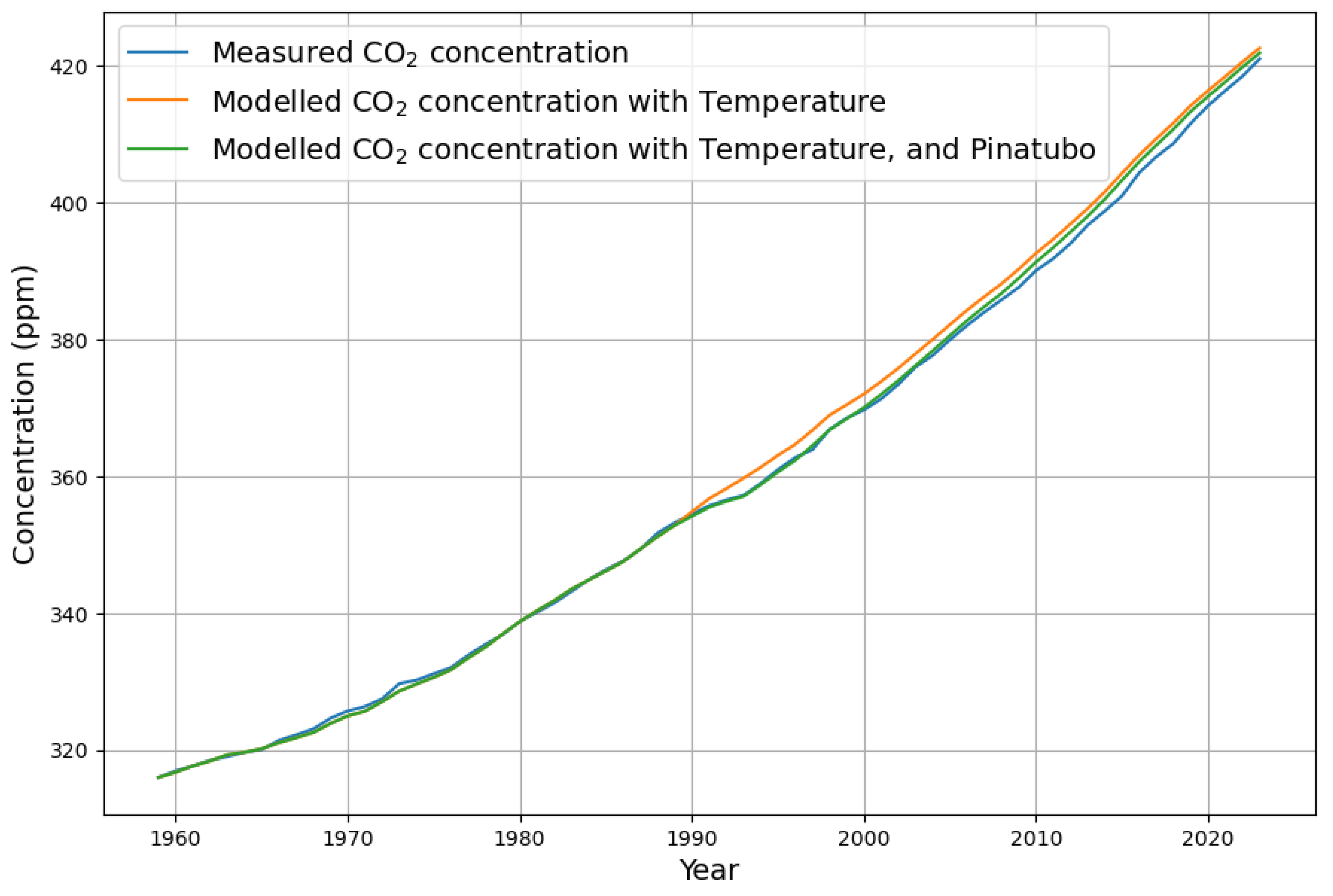
This evaluation is confirmed when looking at the reconstruction in Figure 9. The reconstruction only deviates at 1990 due to the missing sink contribution from the Pinatubo eruption, but follows the shape of the concentration curve precisely. This is an indication that the Concentration+Temperature model is better suited to model the ${\mathrm{CO}}_2$-concentration. In order to compensate the deviations after 1990, the sink effect due to Pinatubo ${\mathrm{A}}_i^P$ must be considered. It is introduced as a negative emission signal, i.e., an additional sink into the recursive modelling equation:

$${\widehat{C}}_i={\widehat{C}}_{i-1}+E_i-A_i^P-{\widehat{S}}_i$$

(19)

This reduces the deviations of the model from the measured concentration significantly according to the green graph in Figure 9. And the understanding of the processes shaping concentration is greatly enhanced. Nevertheless, the model overestimates the ${\mathrm{CO}}_2$ concentration slightly after 2005. It looks that if the natural sinks have a trend at all, it must be a trend to increase the sink effect in recent years rather than saturation.

5.3. Consequences of the Temperature Dependent Model

The concentration-dependent absorption parameter is now in fact more than twice as large as the original absorption parameter of the temperature-independent model, and increasing temperature increases natural emissions. As long as temperature is correlated to ${\mathrm{CO}}_2$ concentration, the two trends cancel each other out, and the sink effect coefficient appears invariant with respect to temperature.

The extended model becomes relevant when temperature and ${\mathrm{CO}}_2$ concentration diverge.

If temperature rises faster than according to the described ${\mathrm{CO}}_2$ proxy relation in Equation (12), then we can expect a reduced sink effect, while with temperatures below the expected value of the proxy the sink effect will increase.

As a first hint for further research, we can estimate the temperature equilibrium concentration based on current measurements. This is given by (anthropogenic emissions and concentration growth at 0 by definition)

$$\begin{array}{ccc}\hfill a·C+b·T+c& =& \hfill 0\hfill \end{array}$$

(20)

$$\begin{array}{ccc}\hfill C& =& \hfill \frac{-b·T-c}{a}\hfill \end{array}$$

(21)

For temperature anomaly $T=0^{\circ }$ (=14 °C worldwide average temperature), the no-emissions equilibrium concentration would be

$$C^{T=0}=\frac{-c}{a}=\frac{13.6}{0.0436}\mathrm{ppm}=312\mathrm{ppm}$$

(22)

The temperature sensitivity is the Change of the zero-emissions equilibrium concentration for 1° temperature change:

$$\frac{\Delta C}{\Delta T}=\frac{-b}{a}=\frac{2.9}{0.0436}\frac{\mathrm{ppm}}{°}=66.5\frac{\mathrm{ppm}}{°}$$

(23)

Rewriting the sink model as

$$\widehat{S_i}=a·(C_{i-1}-C^0)+b·(T_i-T^0)$$

(24)

and taking $C^0=280\mathrm{ppm}$ as the pre-industrial reference concentration, the corresponding reference temperature anomaly $T^0$ was, according to Equation (23),

$$T^0=\frac{a·C^0+c}{b}=-0.{48}^{\circ }.$$

(25)

Obviously, this corresponds very well to the measured data. It must be stated, however, that we derived this result from a time series that is very short in relation to the time constants involved in the underlying processes. All we know about the temperature dependence for sure is that it explains very nicely the short time variability (2.5 years) of the sink effects. From the sign of the temperature coefficient b, we know that it characterizes an emission process, most likely the upwelling advection in warm ocean water. Assuming that the downwelling advection in the cold ocean experiences smaller amplitudes of short term temperature changes but the same longterm trend, then on a short time scale there would be a temperature discrepancy between upwelling and downwelling advection, but not on a long time scale. This is subject to further investigation.

5.4. Does Temperature Dependence Help for Predictions?

When making predictions with a model, it is necessary to know or assume the input data in order to compute a predicted outcome. With the simple linear model only, an emission scenario was required. But with the temperature-dependent model, an assumed temperature is also required. The fact is that temperature is less predictable than ${\mathrm{CO}}_2$ emissions. The best guess we can currently make is that temperature approximately follows the ${\mathrm{CO}}_2$ concentration as it has done for the last 70 years. But then, we know that we cannot discriminate the temperature dependence of concentration growth from concentration dependence. And the remaining zero mean cyclic temperature changes are neither known for the future nor do they have significant influence on the concentration trend.

Therefore, we conclude that there is no point in including temperature explicitly in a prediction of future concentration. The simple linear model without temperature dependence has the same predictive quality.

5.5. Future Emission Scenarios

In order to make predictions, assumptions about future ${\mathrm{CO}}_2$ emissions have to be made. Obviously there are the standard scenarios of IPCC AR6 as a possible first choice [33]. They have, however, severe handicaps. Originating from the time of exponential emission growth, at least 2 IPCC scenarios (SSP5-8.5 named “Avoid at all costs” and SSP3-7 named “Dangerous”) are so far from reality and even from the availability of fossil fuel resources that it is not meaningful to discuss them. For more than the last 10 years, global emissions have been constant within the range of error [29]. This knowledge is not yet reflected adequately in official emission statistics, but also in these statistics there are no significant global emission changes since 2018.

Therefore, approximately constant emissions have to be considered as the worst-case scenario in the real world. This is slightly above the IPCC scenario SSP2-4.5 named “Middle of the road” during the second half of this century.

At the other end of the scale, the IPCC scenario SSP1-1.9 named “Most optimistic” is equally in denial of reality, because it assumes global emissions will to be cut to zero by 2050. None of the large countries that dominate global emissions has any plans to reduce missions to zero [34,35]. Also, SSP1-2.6 named “Next best”, with zero emissions after 2050, ignores industrial transition times, even if there was the political will. Both these scenarios ignore the stabilizing effect of natural carbon sinks, which is the key message of this paper.

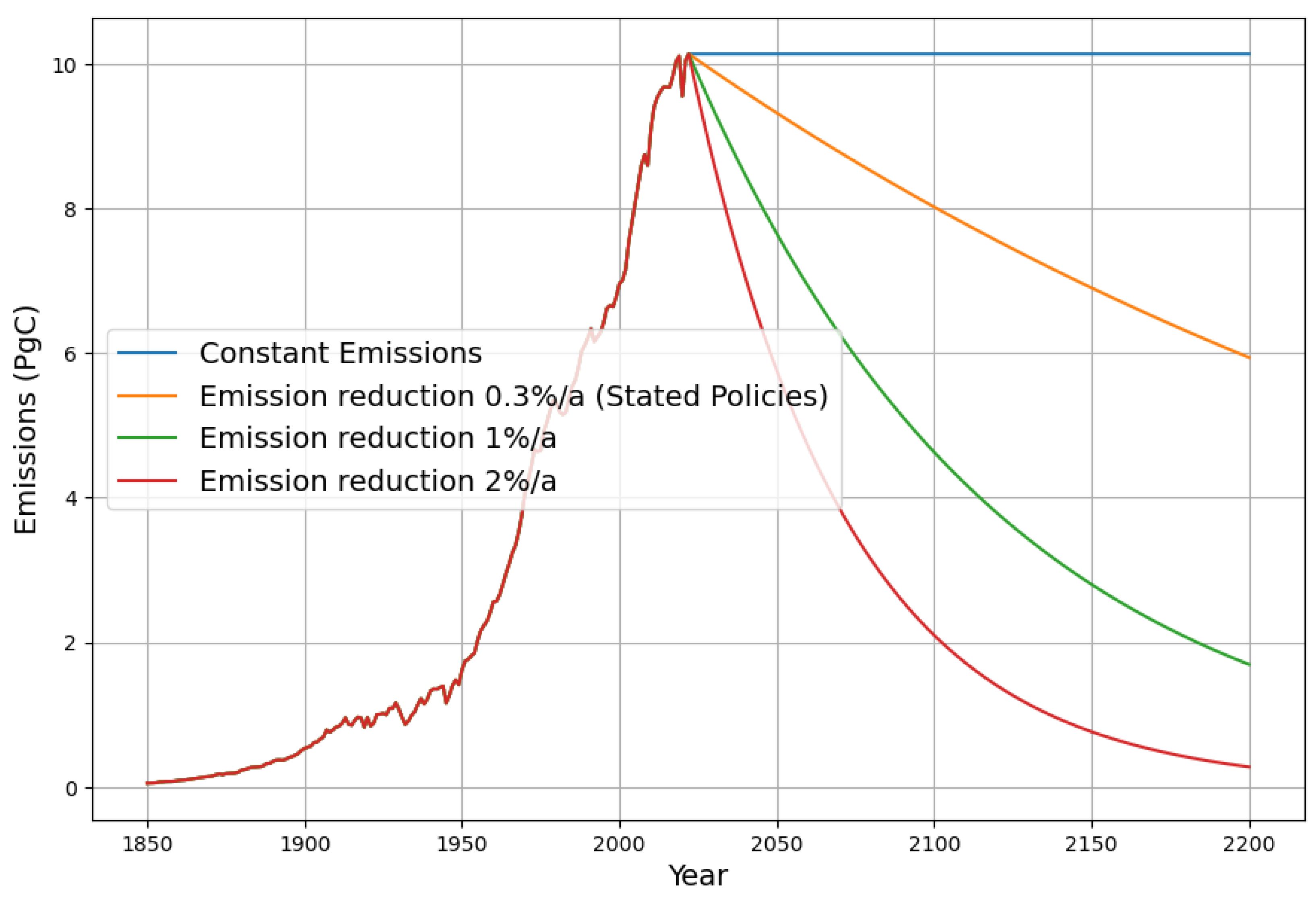
Therefore, I want to focus on four scenarios, displayed in Figure 10, which are less restrictive than SSP1-2.6. First, the mentioned worst-case reference scenario with constant future emissions, extrapolating the recent 5 years.

Then, the IEA “Stated Policies” scenario [36], which is the most likely future emission scenario according to extensive research about existing policy decisions, approximately reducing worldwide carbon emission by 0.3% per annum after 2040. This, in fact, corresponds closely to the IPCC SSP2-4.5 emission scenario.

A more severe emission reduction scenario would be 1% per annum, reducing worldwide emissions by 50% every 70 years, and finally the most aggressive reduction scenario with 2% reduction per annum, reducing emissions by 50% every 35 years. This comes close to the SSP1-2.6 “Next best” scenario without reducing to zero completely.

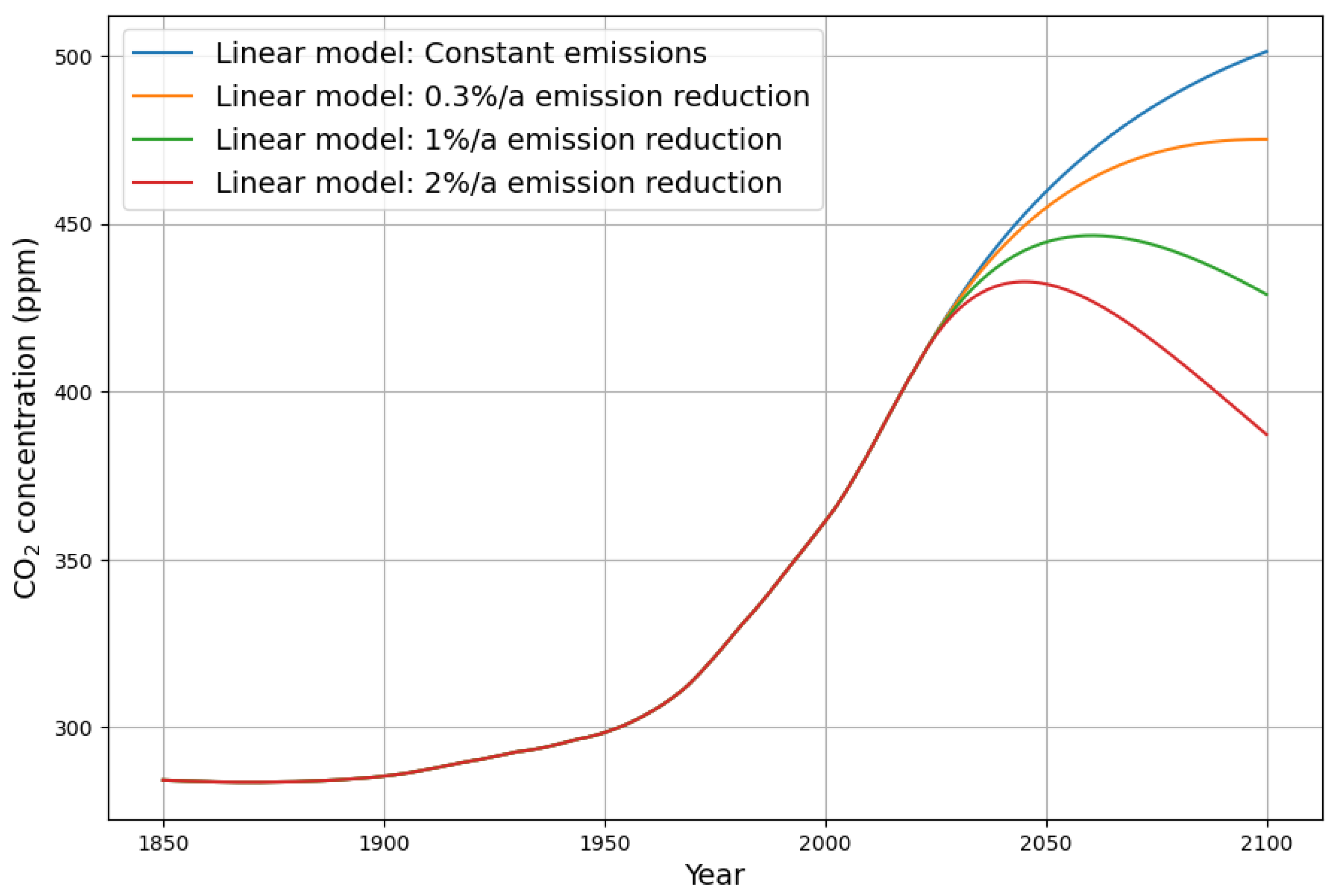
The predictions on the basis of the discussed linear carbon sink model for all four scenarios are shown in Figure 11. With the linear model, all four emission scenarios will not raise the ${\mathrm{CO}}_2$ concentration beyond 520 ppm, and the three emission reduction scenarios will reach the peak concentration within this century. I do not draw conclusions about consequences for global temperature here, because the difficult question of climate sensitivity is clearly beyond the scope of this paper.

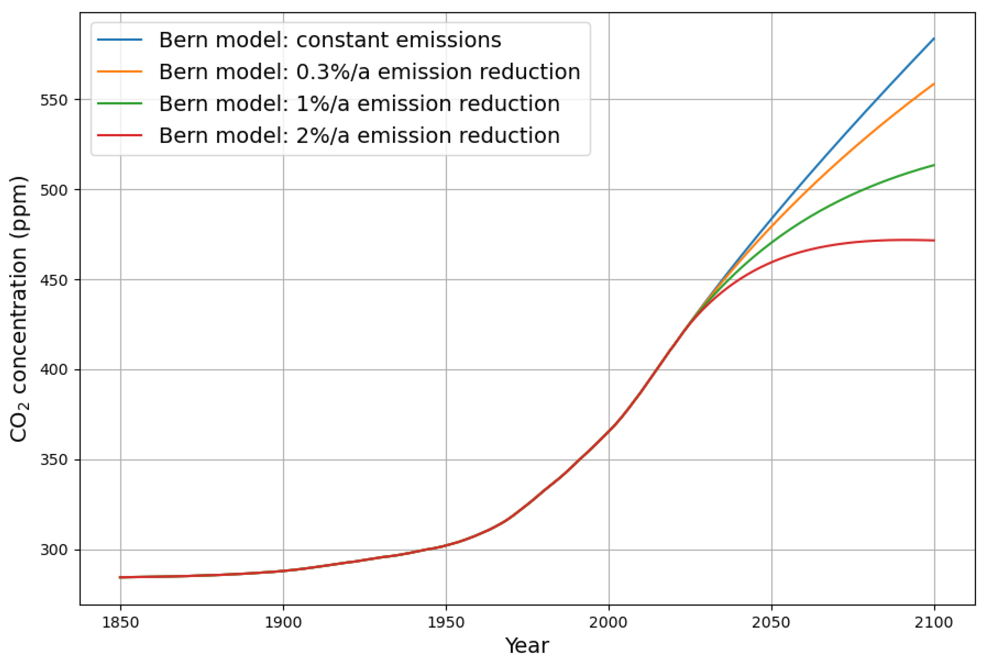
For future historians, I include Figure 12 in order to be able to compare the same scenarios, when the ${\mathrm{CO}}_2$ concentration predictions after 2022 are from the Bern model with the model parameters of 2013 [6]. The IPCC predictions are based on similar models to the Bern model, with comparable outcomes.

The prediction result of the 1% per annum reduction scenario from the Bern model corresponds to the constant emissions prediction scenario result from the linear sink model, and the 2% per annum reduction scenario from the Bern model corresponds to the 0.3% reduction scenario from the linear sink model. Therefore, the question of which model is correct greatly affects future policy decisions.

Within the next 10 to 20 years, it will be easier to see which model will come closest to reality. Until then, the prediction results are similar.

6. A Computational Model for the Vostok Ice Core Data

The Vostok ce core data [37] provide a more than 400,000-year view into climate history, with several cycles between ice ages and warm periods.

Most researchers agree that ${\mathrm{CO}}_2$ data are lagging temperature data by several centuries. One difficulty arises from the necessity that ${\mathrm{CO}}_2$ is measured in gas bubbles, whereas temperature is determined from a deuterium proxy in the ice. Therefore, there is a different way of determining the age for the two parameters—for ${\mathrm{CO}}_2$, there is a “gas age”, whereas the temperature series is assigned an “ice age”. There are estimates of how much older the “ice age” is in comparison to the gas age. But, there is uncertainty, so we will have to tune the relation between the two time scales.

In 2005, several teams made attempts to provide a model of the Vostok data [38]. There was no clear final result, not even about the causality question between temperature and ${\mathrm{CO}}_2$ concentration, although seven of the eight teams preferred temperature to be the cause of ${\mathrm{CO}}_2$ concentration changes, rather than the other way round.

It is difficult to assess the quality of their ${\mathrm{CO}}_2$ reconstruction from the provided figures, and no statistical quality assessment is given. And, from the description, it can be assumed that only the team proposing ${\mathrm{CO}}_2$ to be the cause of temperature changes used a similar model to the one used for investigating the current climate.

6.1. Preprocessing the Vostok Data Sets

In order to perform model-based computations with the two data sets, the original data must be converted into equally sampled data sets. This is done by means of linear interpolation. The sampling interval is chosen as 100 years, which is approximately the sampling interval of the temperature data set. Apart from this, the data sets must be reversed, and the sign of the time axis must be set to negative values.

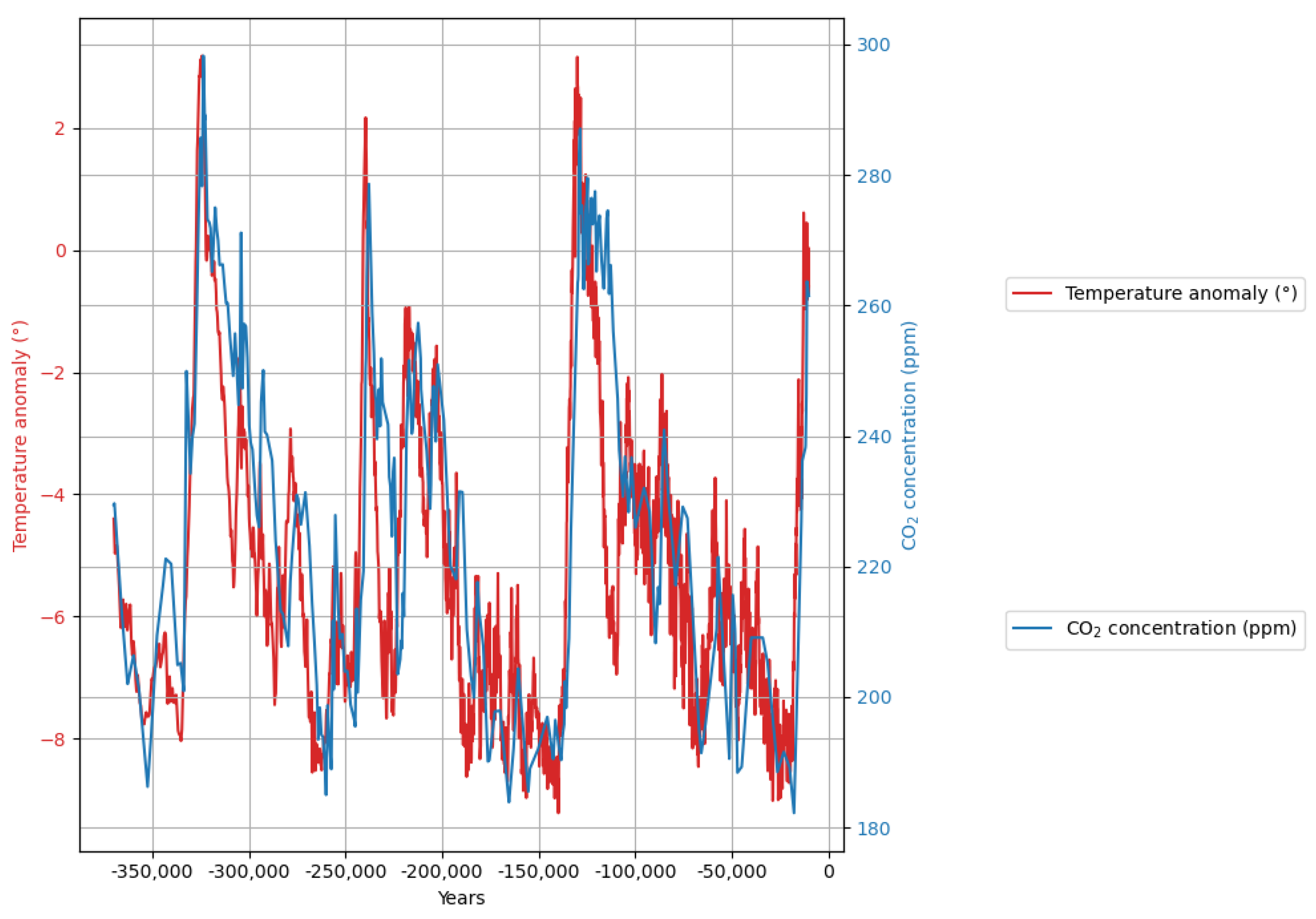
The two re-sampled data sets are shown superimposed in Figure 13.

6.2. Data Model

Due to the fact of the very good predictive quality of the temperature-dependent sink model for current emissions, concentration, and temperature data according to Equation (11), we will use the same model based on ${\mathrm{CO}}_2$ mass balance, and the possible linear dependence of ${\mathrm{CO}}_2$ changes on concentration and temperature, but obviously without any anthropogenic emissions. Also, the time unit is no longer a single year, but a century.

$G_i$ is growth in ${\mathrm{CO}}_2$-concentration $C_i$ during century i given by Equation (1).

$T_i$ is the average temperature during century i. The model equation without anthropogenic emissions is with the estimated sink ${\widehat{S}}_i$ defined as in Equation (11)

$$-G_i={\widehat{S}}_i$$

(26)

After estimating the three parameters a, b, and c from $G_i$, $C_i$, and $T_i$ by means of ordinary least squares, the modelled ${\mathrm{CO}}_2$ data $\widehat{C_i}$ are recursively reconstructed by means of the model, the first actual concentration value of the data sequence $C_0$, and the temperature data:

$$\begin{array}{ccc}\hfill {\widehat{C}}_{-1}& =& \hfill C_{-1}\hfill \end{array}$$

(27)

$$\begin{array}{ccc}\hfill {\widehat{C}}_i& =& \hfill {\widehat{C}}_{i-1}-{\widehat{S}}_i\hfill \end{array}$$

(28)

6.3. Reconstructed ${CO}_2$ Data

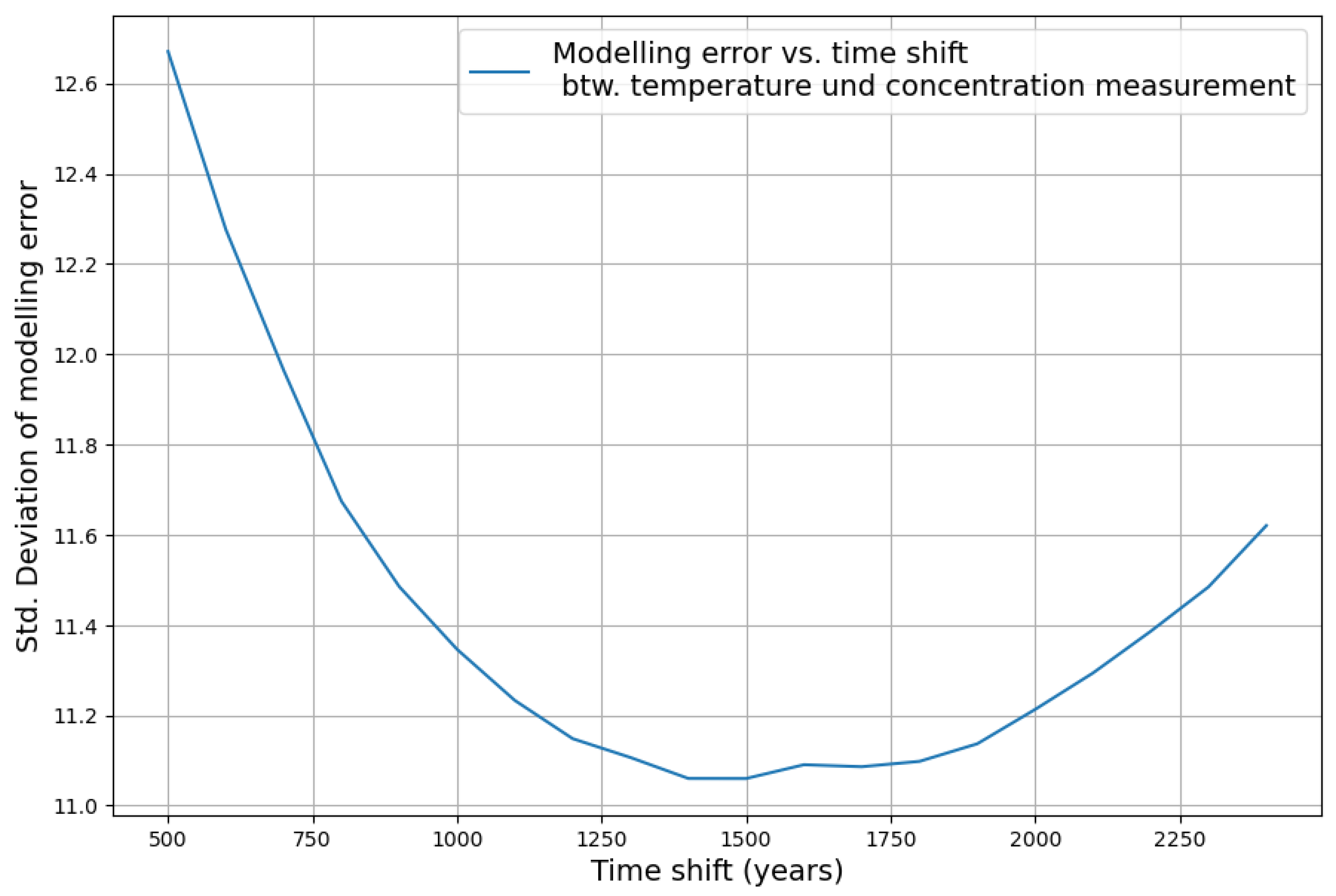
The standard deviation of $\{\widehat{C_i}-C_i\}$ measures the quality of the reconstruction. The standard deviation is minimized, when the temperature data is shifted 1450–1500 years to the past as displayed in Figure 14.

The corresponding estimated model parameters with their significance measures and value range are calculated with the Python OLS package and displayed in

Table 1. Estimated model parameters with significance measures for VOSTOK ice core time series.

	Coef.	Std. Err.	t	$\mathit{P}>\left|\mathit{t}\right|$	[0.025	0.975]
a	0.0133	0.0009	15.3	0.0000	0.0116	0.0149
b	−0.1799	0.0086	−20.8	0.0000	−0.1968	−0.1630
c	−3.8965	0.2298	−17.0	0.0000	−4.3471	−3.4458

.

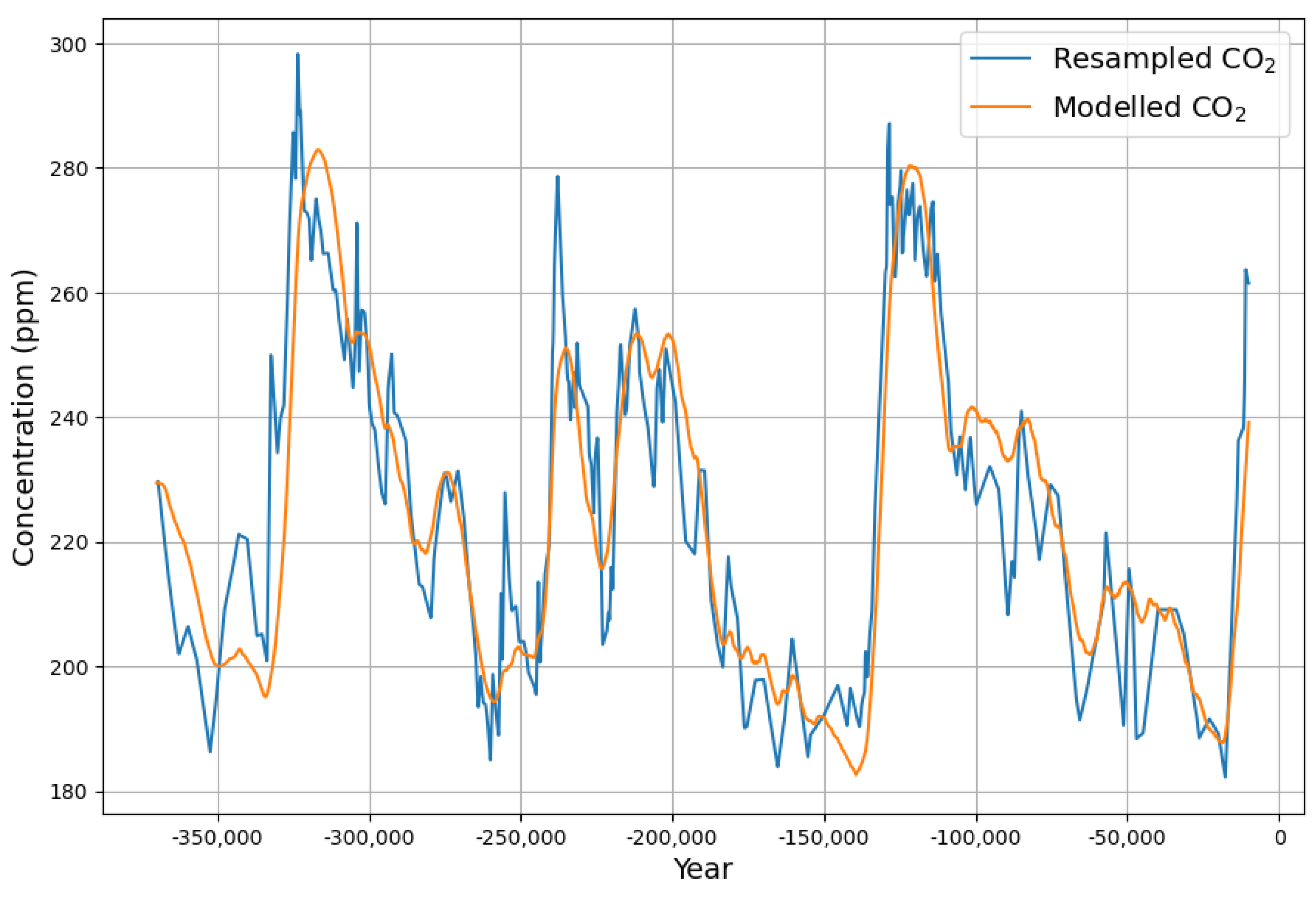
The interpretation is that there is a carbon sink of 1.3% per century, an emission increase of 0.18 ppm per century, and a 1 degree temperature increase. The reconstruction of ${\mathrm{CO}}_2$ data from the temperature-extended sink model looks quite remarkable, as displayed in Figure 15.

6.4. Equilibrium Relations

The equilibrium states are more meaningful than the incremental changes for such “distant” data. The equlibrium is defined by equality of ${\mathrm{CO}}_2$ sources and sinks, resulting in $G_i=0$. This creates a linear relation between ${\mathrm{CO}}_2$ concentration C and Temperature T:

$$C=\frac{0.1799·T+3.8965}{0.0133}\mathrm{ppm}$$

(29)

For the temperature anomaly $T=0$ we therefore obtain the ${\mathrm{CO}}_2$ concentration of

$$C_{T=0}=\frac{3.8965}{0.0133}\mathrm{ppm}=293\mathrm{ppm}$$

(30)

The difference of this to the modern data can be explained by different temperature references. Both levels are remarkably close, considering the very different environmental conditions.

And the temperature sensitivity of concentration at equilibrium is

$$\frac{dC}{dT}=13.5\frac{\mathrm{ppm}}{°\mathrm{C}}$$

(31)

This is considerably different from the modern data, where we obtained $66.5\frac{\mathrm{ppm}}{°\mathrm{C}}$. As stated above, it is possible that this high value is restricted to rather short time intervals of a few years and gets smaller when the data are integrated over time. This effect can be observed qualitatively when the measured data are smoothed. A reviewer of this paper pointed out that this discrepancy could have its cause in the added carbon in the atmosphere as well as in the mixed layer of the ocean. If the negative temperature dependency of the carbon sink effect is mainly from the upwelling advection, then it might be possible that the temperature-dependent changes are also dependent on the concentration and temperature of the mixed layer and their relation to these properties in the atmosphere, both of which have changed considerably since the rise in both temperature as well as ${\mathrm{CO}}_2$ concentration during the last 170 years. It must be stated, however, that we cannot simply attribute the high equilibrium value as a consequence of the greenhouse effect, because that would reverse the causal direction of the effect.

Therefore, we have reason to assume that the lower value of $13.5\frac{\mathrm{ppm}}{°\mathrm{C}}$ represents the true longterm sensitivity of ${\mathrm{CO}}_2$ concentration from temperature.

7. Conclusions

The purpose of this paper is to discover and evaluate more subtle aspects of the linear sink model published previously.

The apparent inconsistency between the sensitivity of the sink effects to short term temperature variations but invariance with respect to temperature trends has been resolved by identifying the collinearity between temperature trends and ${\mathrm{CO}}_2$ concentration. In particular, during the last 70 years the correlation between temperature and ${\mathrm{CO}}_2$ concentration has been very high. Consequently all temperature trend dependence has been attributed to ${\mathrm{CO}}_2$ concentration in the original linear model. By evaluating the measured data with a model, where the residual temperature is added, the actual temperature dependence can be measured. By this procedure, the model is extended to become truly temperature-dependent. Further research is needed to validate the results of the extended model with other measurements.

For future concentration predictions from emissions, however, the temperature-dependent model does not really help, because the most likely future temperature is already covered in the simple temperature-independent model. This will change, however, if temperature development will deviate from the pattern of the last 70 years.

The temperature-enhanced model also reproduces nicely the ${\mathrm{CO}}_2$ concentrations of the Vostok ice core data series. As a side effect, this confirms that in paleo-climate data series, temperature leads ${\mathrm{CO}}_2$ concentration.

With recent data, where there is a strong correlation between ${\mathrm{CO}}_2$ concentration and temperature, the temperature trend dependence is balanced; therefore, we have to accept that currently the anthropogenic emissions are the main visible driver of atmospheric ${\mathrm{CO}}_2$ concentration, while temperature effectively only adds some zero mean variability.