Article

Climate Classification for Major Cities in China Using Cluster Analysis

1
Shenzhen Institute of Advanced Technology, Chinese Academy of Sciences, Shenzhen 518055, China
2
University of Chinese Academy of Sciences, Shenzhen Institute of Advanced Technology Campus, Beijing 101408, China
3
Water Engineering Department, Faculty of Agricultural Sciences, University of Guilan, Rasht P.O. Box 41889-58643, Iran
*
Author to whom correspondence should be addressed.
Atmosphere 2024, 15(7), 741; https://doi.org/10.3390/atmos15070741
Submission received: 15 May 2024 / Revised: 7 June 2024 / Accepted: 17 June 2024 / Published: 21 June 2024
(This article belongs to the Section Climatology)

Abstract

:
Climate classification plays a fundamental role in understanding climatic patterns, particularly in the context of a changing climate. This study utilized hourly meteorological data from 36 major cities in China from 2011 to 2021, including 2 m temperature (T2), relative humidity (RH), and precipitation (PRE). Both original hourly sequences and daily value sequences were used as inputs, applying two non-hierarchical clustering methods (k-means and k-medoids) and four hierarchical clustering methods (ward, complete, average, and single) for clustering. The classification results were compared using two clustering evaluation indices: the silhouette coefficient and the Calinski–Harabasz index. Additionally, the clustering was compared with the Köppen–Geiger climate classification based on the maximum difference in intra-cluster variables. The results showed that the clustering method outperformed the Köppen–Geiger climate classification, with the k-medoids method achieving the best results. Our research also compared the effectiveness of climate classification using two variables (T2 and PRE) versus three variables, including the addition of hourly RH. Cluster evaluation confirmed that incorporating the original sequence of hourly T2, PRE, and RH yielded the best performance in climate classification. This suggests that considering more meteorological variables and using hourly observation data can significantly improve the accuracy and reliability of climate classification. In addition, by setting the class numbers to two, the clustering methods effectively identified climate boundaries between northern and southern China, aligning with China’s traditional geographical division along the Qinling–Huaihe River line.

1. Introduction

Climate classification is the process of categorizing different areas of the Earth based on meteorological factors, such as near-surface air temperature, precipitation, humidity, wind, and radiation [1,2,3,4]. Among these climate variables, near-surface air temperature and precipitation are the most widely used for climate classification due to their impact and relatively easy data availability [2,3,5]. This classification is crucial for understanding the climatic features of various regions and has significant implications in agriculture, ecology, industry, urban construction, species migration, and even virus spread [6,7].
The traditional Köppen–Geiger method, pioneered in 1900, is based on the knowledge of climatologists, who use statistical data of meteorological elements to manually define classification standards [2,3,8,9,10]. However, this method, with the aim of reflecting different surface vegetation distributions, has errors in expressing actual vegetation distribution boundaries [11]. Moreover, the Earth’s climate is constantly changing. Since the beginning of the industrial era, the global average surface temperature has risen by 1.1 °C, and the rise is uneven across all regions of the world [12]. Therefore, it is necessary to redefine the climate zones with a changing climate pattern.
China, a country spanning a large area, exhibits different environmental and climatic conditions in its northern and southern regions. In 1908, Zhang Xiangwen proposed the ‘Qinling–Huaihe River line’ as the geographic demarcation line between the two regions [13]. This line, characterized by an annual precipitation of 800 mm and serving as the 0 °C isotherm in January, has been widely adopted as a defining boundary due to the substantial differences in temperature, precipitation, drought occurrences, crop types, and terrain between northern and southern China, warranting separate analyses of these regions [14]. Over time, this division has been extensively utilized in studies related to agriculture, environment, and climate in China [14,15,16].
The Köppen–Geiger method divides climate zones according to fixed thresholds. For example, when a region experiences the climate that the average temperature of the hottest month exceeds 22 °C, the average temperature of the coldest month is at or below 0 °C, and the summer’s driest month receives less than one-tenth of the winter’s wettest month precipitation, the Köppen–Geiger method identifies the region as Dwa, representing a humid continental climate [2]. Unlike Köppen–Geiger method, unsupervised data-driven methods, such as k-means, do not require determining thresholds and have shown advantages in statistical performance [17]. Climate classification has begun to use clustering methods [18,19,20,21,22,23], which are particularly well-suited for testing temporal climate zones in the context of diverse climatic variations in different regions [24]. The use of cluster analysis, an unsupervised data-driven method, is highly valuable for research purposes.
Existing research on climate classification has employed various clustering methods, including non-hierarchical and hierarchical clustering. For example, a study in Alabama used three different hierarchical clustering methods, average, centroid, and ward, to cluster weather based on seven meteorological elements [25]. Similarly, the ward hierarchical clustering method and the partitioning around medoids method were applied for global climate clustering analysis and compared with the Köppen–Geiger climate classification [26]. Additionally, k-means and k-medoids have been utilized to develop numerical climate classifications [19]. Furthermore, based on long-term average climate behavior, non-hierarchical k-mean and hierarchical methods, such as single, complete, McQuitty, average, centroid, and median, and two ward methods, wardD and wardD2, were used to categorize the Borneo region into several homogeneous groups, identifying four main climate zones [22]. In a study on the climatic classification of Turkey, five hierarchical clustering methods were employed, demonstrating the likelihood of the ward method to produce acceptable results [27]. Moreover, a study utilized k-means clustering analysis to regionalize Europe based on climate change [28], defining regions with similar average climate and predicted changes in the context of climate change [29].
In China, research on climate classification using clustering methods has been conducted. Based on monthly average temperature and precipitation data from 753 national meteorological stations in China spanning from 1966 to 2005, Zhang et al. [24] used k-means clustering analysis to classify them into ten types. However, due to the unique climate characteristics of the 11 mountainous climate stations in southeastern China, they were classified as a special category. Therefore, this study actually defined nine climate regions [24]. In another study, Shi et al. [4] utilized k-nearest neighbor and sparse subspace representation, then applied spectral clustering to divide 661 meteorological stations in China into several regions. This study used five climate variables, i.e., daily average temperature, average relative humidity, sunshine hours, diurnal temperature range, and atmospheric pressure. The study provided insights into climate classification from both single and multiple perspectives [4]. Furthermore, Bai et al. [30] used three different clustering analysis methods, including k-means, average-linkage, and Ward’s clustering, to develop new thermal climate zones for building energy efficiency by using daily values. The analysis showed that average linkage clustering was more suitable for the study, resulting in higher accuracy for the new region compared with the existing regions, thereby providing more precise climate information [30].
Unlike the previous studies, this study employs hourly meteorological data and six clustering methods to classify the climate of 36 major cities in China. The clustering results are evaluated using two internal evaluation methods, the silhouette coefficient and the Calinski–Harabasz index [31], and are further compared with the traditional Köppen–Geiger method. In addition, the study utilizes a data-driven approach, employing a clustering method with k = 2, to investigate the relationship between the conventional north–south division and the data-driven north–south division. The research objectives are: (1) To investigate the impact of hourly sequences and daily sequences on climate classification; and (2) to examine the effects of utilizing three meteorological elements and two meteorological elements at different temporal resolutions with various clustering methods on climate classification.
The remaining part of the paper is as follows. The data and methods are introduced in the second section. The results and discussion are presented in the third section, and the conclusion is provided in the final section.

2. Materials and Methods

2.1. Study Area and Data

We selected 36 major cities in China as research sites, including 31 provincial capitals and five municipalities directly under the central government’s economic plan. These cities are characterized by high population density, extensive urban development, and advanced infrastructure. According to recent demographic statistics, these 36 cities accounts for approximately 26% of the national population, while their total area occupies only about 5% of the country. Given that these cities serve as the economic, cultural, and transportation hubs locally, understanding the climate characteristics is crucial for long-term regional sustainable development.
Figure 1 illustrates the locations of the 36 basic meteorological stations, revealing that these stations have covered all Chinese provinces, effectively representing the climate of the most densely populated area in each province. The names, abbreviations, provincial affiliations, geographical coordinates, and the altitude of these stations are listed in Table 1. The distribution of these stations, as shown in Figure 1 and Table 1, is uneven across China, with more stations located in eastern China than in the west. This distribution aligns with the demographic concentration highlighted by the Hu Huanyong Line, which delineates the significant population disparity between eastern and western China [32]. Furthermore, Figure 1 and Table 1 show that western China is characterized by rugged terrain, including mountain ranges and high plateaus, while eastern China is marked by low-lying areas, bordering the Bohai Sea (BHS), Yellow Sea (YLS), East China Sea (ECS), and South China Sea (SCS).
The data used in this study consist of hourly observations of 2 m temperature (T2), relative humidity (RH), and precipitation (PRE) from January 2011 to December 2021, provided by the China Meteorological Administration. These data have been quality controlled and are of high quality.

2.2. Methods

2.2.1. Köppen–Geiger Climate Classification

The Köppen–Geiger climate classification is based on calculating the average monthly temperatures and cumulative monthly precipitation over the 12 months of a year [9]. Global climate is divided into five major climate zones: A (Tropical), B (Arid), C (Temperate), D (Cold), and E (Polar), based on latitude, from low to high. Each major category can be subdivided into several subcategories. In this study, we used hourly temperature and precipitation data from the 36 stations from 2011 to 2021 to calculate the monthly average temperature and monthly average cumulative precipitation, following the approach as specified by Peel et al. [2].

2.2.2. Hourly Sequence and Daily Sequence

The original dataset comprises hourly T2, RH, and PRE observations from 1 January 2011 to 31 December 2021, resulting in a dataset with 96,432 × 3 data points. These elements are combined into a single-dimensional dataset, starting with an 11-year T2 series, followed by RH, and finally, hourly PRE. Due to the differing scales of these meteorological elements, we initially normalized them by applying min–max scaling across all stations. For example, we aggregated T2 data from 36 sites, identified the maximum and minimum values, and then normalized these data. The normalization process is described by the following formula [24]:
X i t p = X i t p min X i max X i min X i ,
where i = 1,2 , 3 represents hourly T2, RH, and PRE, respectively, and X i t p represents the observed value of a certain meteorological factor at time t   at p meteorological stations. X i represents all observed values of the i-th meteorological factor at all stations during the study period. Normalization ensures that different meteorological factors contribute equally to the clustering calculation, regardless of variations in their value ranges or magnitudes.
Previous studies typically rely on monthly averages derived from daily sequence values for climate classification, including daily maximum, minimum, and average values. In contrast, this study normalizes hourly data and directly uses clustering methods for climate classification, utilizing high-resolution time-series information. We compared the results directly derived from hourly data with the clustering results using daily sequences, obtained by calculating daily maximum, minimum, and average values from hourly data.

2.2.3. Clustering Method

Clustering, an unsupervised learning method, involves organizing unlabeled data points into groups based on their similarities, aiming to identify inherent structures or patterns within the data [33]. Hierarchical and non-hierarchical methods are two commonly used clustering methods [34,35,36]. In this study, four hierarchical clustering methods and two non-hierarchical clustering methods are employed to categorize the climate type for the 36 stations.
Non-hierarchical clustering methods include k-means clustering and k-medoids clustering. In the k-means algorithm, given a set of points, x 1 , x 2 , … x m , to be classified into k classes, C = C 1 , C 2 , , C k , the objective is to minimize the summation of squared errors within the same group, which is defined as follows [36]:
J = j = 1 k i = 1 m x i j μ j 2 ,
where μ j is the mass center of cluster C j , representing the average vector of all points within the cluster, and x i j indicates that point i belongs to cluster C j . In this study, where m   = 36, we employed the non-hierarchical clustering methods, including k-means and k-medoids clustering. The value of k, an external parameter in clustering algorithms, is determined by referring to the Köppen–Geiger climate classification result, which categorizes the meteorological stations into certain classes. For the initialization of cluster centers in the k-means algorithm, the enhanced k-means++ algorithm was utilized to stabilize the clustering outcome. The process begins by randomly selecting a point from the dataset as the first center. Subsequently, for each point in the dataset, the distance to the nearest center was calculated and a new center was selected with a probability proportional to the square of the distance to the already chosen center. This process was repeated until k centers were all selected [37].
The k-medoids clustering method, similar to k-means, is a prototype-based clustering approach that seeks representative points for each cluster. Unlike k-means that uses the mass center of a cluster, k-medoids employs an actual central point within the cluster, which is the point with the minimum total distance to all other points in the cluster [38]. While k-medoids offers better robustness against outliers, it requires significantly more computational effort compared with k-means, especially when dealing with a large number of points, as selecting actual central points is more time-consuming than calculating centroids. In our study, the distance metric employed is the Euclidean distance, the most commonly used distance measure in clustering algorithms [27].
In our study, we utilize the agglomerative clustering algorithm for hierarchical clustering, which operates from the bottom up. This method considers each sample as an initial cluster, resulting in m clusters for m samples. At each step, the algorithm identifies and merges the two nearest clusters, continuing this process until the predetermined number of clusters is reached. For the ‘linkage’ parameter in hierarchical clustering, our research selects four methods: ‘ward’, ‘average’, ‘complete’, and ‘single’ [39,40,41]. The ‘ward’ method aims to minimize the total variance in each cluster when merged with other clusters; ‘average’ calculates the mean distance from a point in one cluster to all points in another cluster; ‘complete’ uses the maximum distance between points in two clusters; and ‘single’ calculates the minimum distance from a point in one cluster to all points in another cluster and then takes the minimum of these distances [39,40,41]. In hierarchical clustering, once the points are classified into a particular cluster, they will not be reassigned and will always remain in that cluster. In contrast, non-hierarchical clustering allows for the reassignment of points to different clusters during each iteration, making it more flexible.

2.2.4. Clustering Evaluations

Evaluating clustering performance is crucial for clustering analysis, providing insights into the effectiveness and optimization of clustering algorithms. However, a clustering evaluation without pre-existing labels remains a challenging problem [42]. Typically, there are two types of clustering evaluation methods: an external evaluation, which relies on external information, such as predefined labels or classifications, and internal evaluation, which assesses clustering results independently. This research has no strict and unified definition for climate classification, so an external evaluation is not feasible. Consequently, this study focuses on the internal evaluation, utilizing two common indices, the silhouette coefficient and Calinski–Harabasz index. These indices mainly consider intra-class compactness and inter-class separation for clustering, assessing the samples’ proximity within the same class and the distinction between different classes [31].
The calculation method for the silhouette coefficient is as follows. For a sample point, j, belonging to class C i , its silhouette coefficient is calculated using the following formula [43]:
S j = b j a j max b j , a j ,
where a ( j ) represents the average distance between the sample point, j, and other points in the class, C i ,
a j = 1 n i l = 1,2 , , n i ; l j d x j , x l .
Here, d x j , x l refers to the distance between sample point x j and x l ; n i is the number of samples of class C i . The minimum average distance from sample point j to all other classes of C h ( h = 1,2 , , k ; h i ) is expressed as [43]:
b j = min h = 1,2 , , k ; h i 1 n h x l C h d x j , x l .
Here, n h is the number of samples of class C h . After calculating all the sample points, the average silhouette coefficient ( S C ) of clustering is [43]:
S C = j = 1 N S j N ,
where N is 36 in this study, and the SC ranges from −1 to 1, with values closer to 1 indicating better clustering, greater compactness within the class, and better separation between classes.
The calculation formula for the Calinski–Harabasz index is as follows [43]:
C H = T r S B k 1 T r S w n k ,
where T r S B is a covariance matrix between classes; T r S w is a covariance matrix of in-class data, and they can calculated as follows [43]:
T r S B = i = 1 k n i × d v i , v ¯ ,
T r S w = i = 1 k j = 1 n d x j , v i ,
where n i is the sample’s class number, i ; v i is the center of each class; v ¯ is the center of all samples; and the range of the CH index is (0, +∞). A larger CH index indicates better clustering.

3. Results and Discussions

3.1. Köppen–Geiger Climate Classification

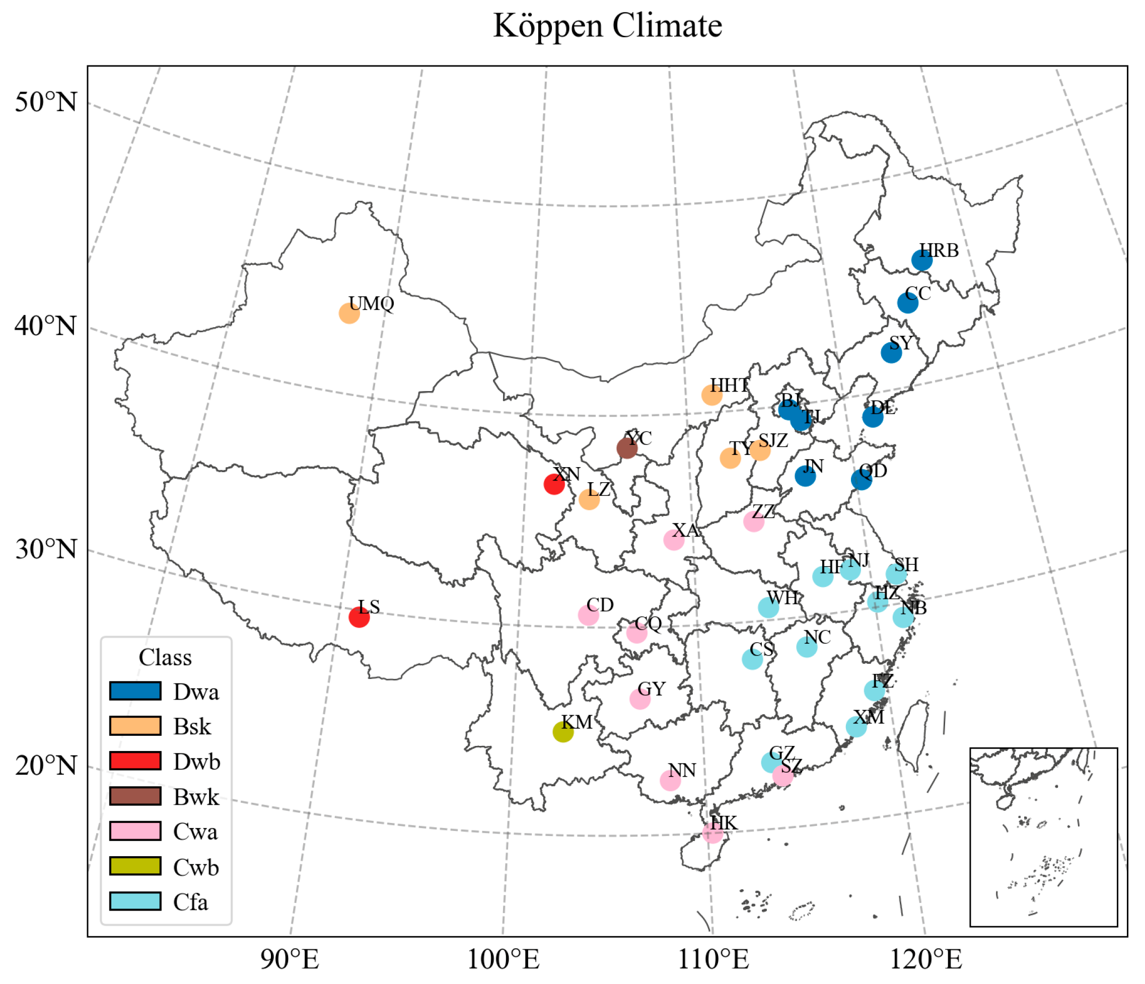
Based on the hourly meteorological data from 2011 to 2021, average monthly T2 and monthly cumulative PRE are calculated to classify the climate type in the 36 major cities in China using the Köppen–Geiger climate classification method. This results in classifying these cities into seven distinct climate types, as shown in Figure 2. As mentioned in the Methodology Section, 7 is therefore utilized as an external parameter for subsequent clustering computing.
China is divided geographically by the Qin Mountains and the Huai River line [13], forming 15 northern and 19 southern provinces and municipalities directly under the central government. Figure 2 shows that most of the northern cities exhibit Dwa and Bsk climate types, representing humid continental and continental semiarid climates, respectively. Notably, Yinchuan, the capital city of Ningxia province, is classified as Bwk, referring to a cold desert climate due to its desert location and wide temperature range. In contrast, southern cities are mainly characterized by a humid subtropical climate (Cfa) or a monsoon-influenced humid subtropical climate (Cwa). Kunming (the capital city of Yunnan province) stands out as a subtropical highland climate (Cwb), and Lhasa, located on the Tibet Plateau, has a complex climate classified as a warm-summer humid continental climate (Dwb).
However, the Köppen–Geiger climate classification method has some limitations. For instance, it classifies the climates of Haikou and Shenzhen as the same as those of Zhengzhou and Xi’an (Figure 2), which is not in line with people’s perceptions. Xi’an and Zhengzhou have four distinct seasons, while Haikou and Shenzhen have very long summers and almost no winter.

3.2. Non-Hierarchical Clustering Results Based on the Hourly Sequence

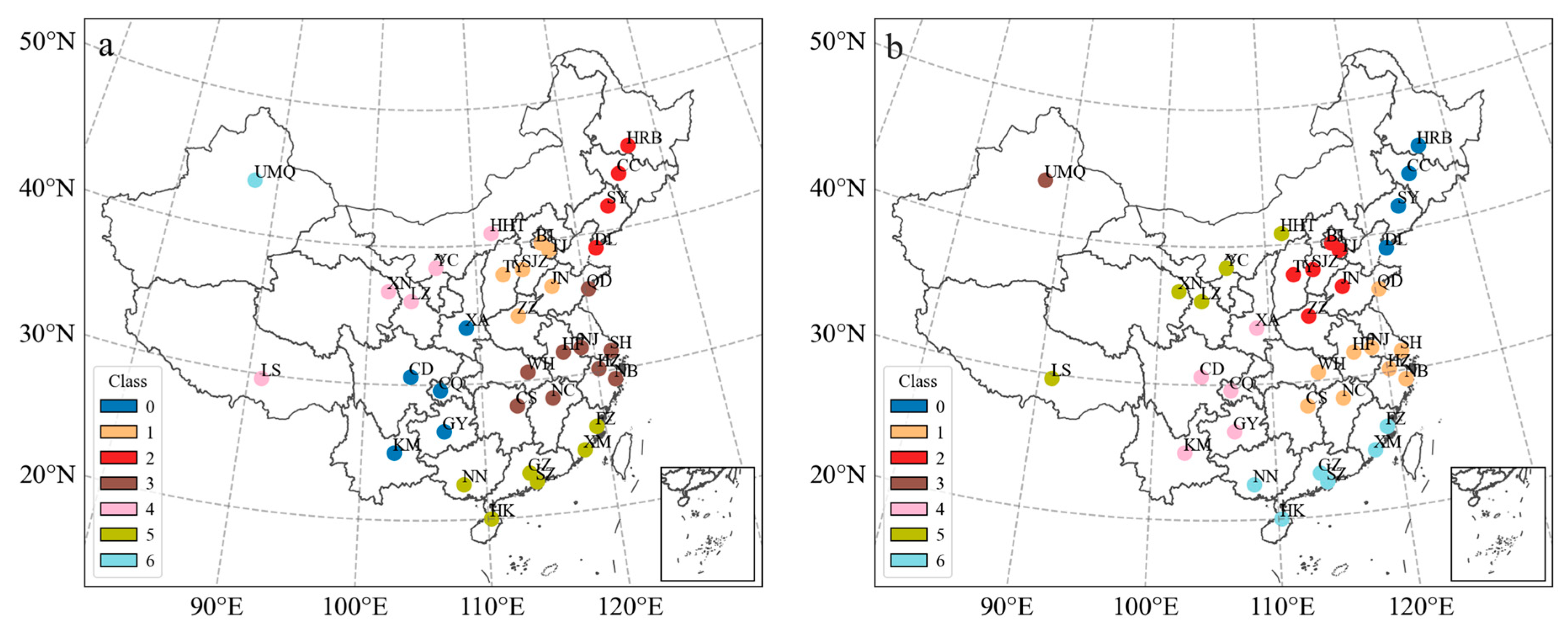
Based on the non-hierarchical clustering k-means and k-medoids methods by using hourly T2, RH and PRE observations from 2011 to 2021, the clustering results for the 36 stations are shown in Figure 3. The categories are denoted by ordinal numbers 0, 1, …, 6, consistent with all later clustering results in this study.
The results in Figure 3 show that k-means and k-medoids clustering methods achieve identical results when applied to the hourly data. Non-hierarchical clustering groups Lhasa and several cities in the northwest region, such as Xining, Lanzhou, Yinchuan, and Hohhot, are placed into one category, while cities in the Northeast region (Harbin, Changchun, Shenyang, and Dalian) are classified together. Urumqi is segregated into a separate category, demonstrating its unique climate characteristics.
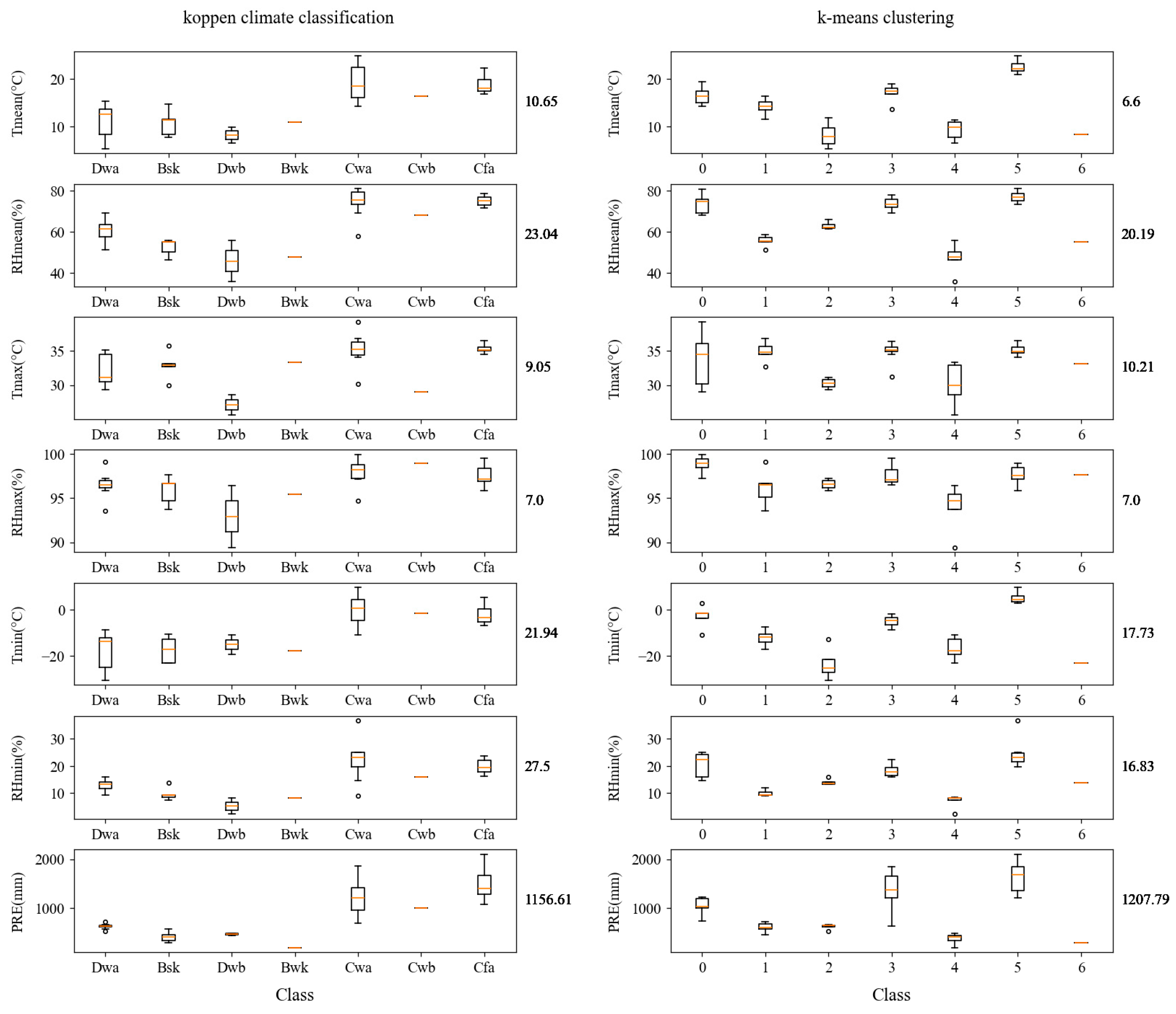
In order to compare the effectiveness of the Köppen–Geiger classification with k-means and k-medoids clustering, seven climate variables are selected to assess the maximum differences within the same category. These variables include annual average temperature ( T m e a n ) and relative humidity ( R H m e a n ), average annual maximum and minimum temperatures ( T m a x and T m i n ) and relative humidity ( R H m a x and R H m i n ), and annual accumulated precipitation ( P R E ). The box plots in Figure 4 demonstrate the climate variable values of the stations within each category. The value on the right side of each sub-plot represents the maximum difference in climate variables between stations within the same category. A smaller difference indicates a more effective classification. Since the two non-hierarchical clustering results are the same, only k-means is used for comparison with the Köppen–Geiger climate classification.
Based on the values shown to the right of each sub-plot in Figure 4, it can be seen that the maximum intra-class differences in climate variables of T m e a n , R H m e a n , T m i n , and R H m i n for categories classified by the k-means method are smaller than the those classified by the Köppen–Geiger climate classification method. The maximum intra-class differences in T m a x and annual cumulative P R E for categories classified by the k-means method are larger than those classified by the Köppen–Geiger climate classification method, while for R H m a x , the maximum intra-class differences are equal for both methods. Therefore, the k-means classification method is superior to the Köppen–Geiger method for climate classification in this study, showcasing smaller maximum differences in most of the climate variables within each subdivision.
The behavior observed in Figure 4 can be attributed to the fundamental principles underlying the two classification methods. The objective function of k-means clustering, as shown in Equation (2), explicitly aims to minimize the sum of squared errors between each data point and the centroid of its assigned cluster. This approach ensures the creation of clusters with minimized intra-class differences, resulting in more homogeneous clusters regarding the considered climate variables. In contrast, the Köppen–Geiger classification method relies on predefined thresholds and categorical boundaries based on empirical rules. While effective for general climate classification, these fixed thresholds do not adapt to the specific distribution of the dataset being analyzed, potentially leading to larger intra-class differences.

3.3. Hierarchical Clustering Results Based on the Original Sequence

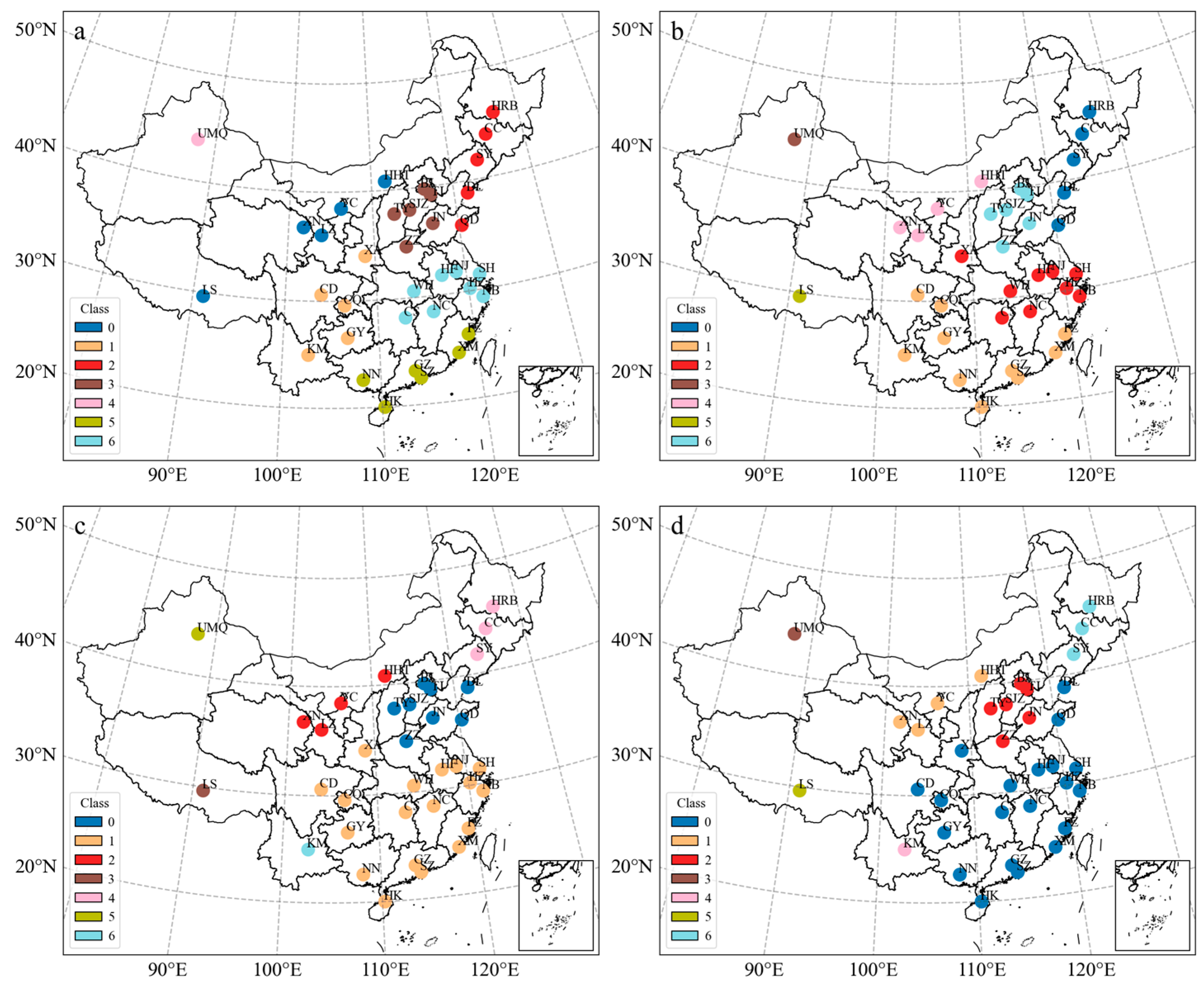
This study further employs a hierarchical clustering method using four linkage methods: ward, complete, average, and single. These methods are utilized to classify the original hourly T2, RH, and PRE sequences, and the classification results are shown in Figure 5. It is worth noting that the hierarchical clustering methods of the four linkage methods produce different classification results.
The results obtained from the ward hierarchical clustering method closely resemble those obtained from non-hierarchical clustering, with the exception of Qingdao, which is located at the boundary between two categories. Among the four hierarchical clustering results, the average and single methods demonstrate relative similarity. Both methods delineate Urumqi, Lhasa, and Kunming as separate categories, while forming a large cluster in southern China. The average cluster includes 18 sites, whereas the single cluster in southern China encompasses 20 sites. In the context of aggregated hierarchical clustering algorithms, some linkage methods are prone to a phenomenon often referred to as “the rich getting richer” [44], where merged clusters are more likely to absorb other clusters. This tendency is notably observed in the average and single methods, especially in the single distance strategy. These methods often result in larger clusters, leading to more imbalanced clustering outcomes.

3.4. North and South Climate Classifications Based on Hourly Meteorological Observations

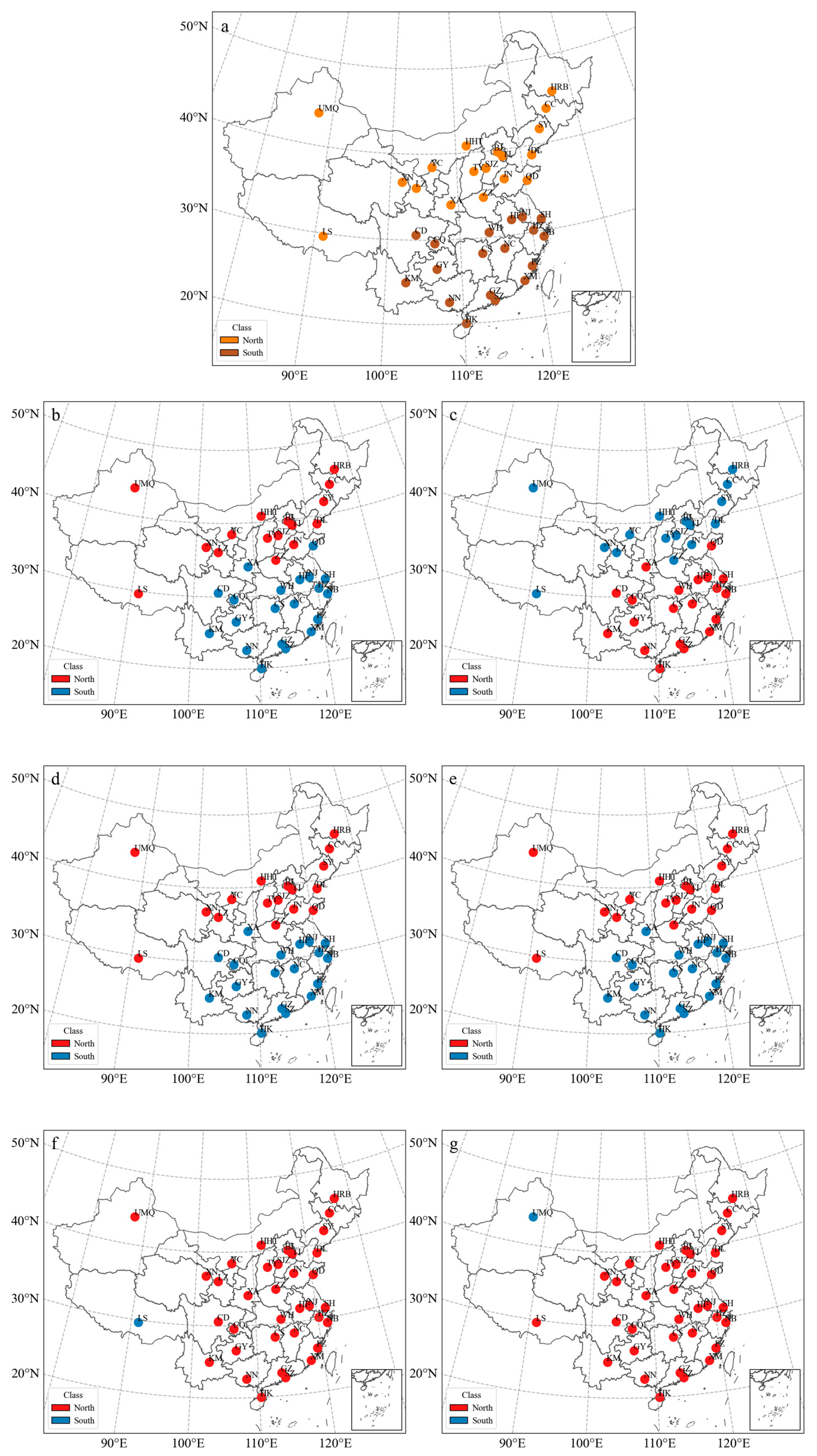
Traditionally, China has been geographically divided into northern and southern regions along the Qinling–Huaihe River line, which approximates the 0 °C January isotherm and the 800 mm isohyet in China [10,11] (Figure 6a). In this study, two non-hierarchical clustering methods (k-means and k-medoids) and four hierarchical clustering methods (ward, complete, average, and single) are employed to categorize the 36 cities using k = 2, based on hourly meteorological observational data from 2011 to 2021. The results are shown in Figure 6b–g. The choice of k = 2 aims to investigate whether the two types derived from data-driven classification align with the traditional northern and southern regional divisions of China.
The k-means and k-medoids methods produce identical outcomes (Figure 6b,c), differing from the traditional north–south classification along the Qinling–Huaihe River line for two cities, Xi’an and Qingdao, which are classified as southern cities. The hierarchical clustering methods, ward and complete approaches (Figure 6d,e), produce the same results and differ from the traditional north–south classification for one city, categorizing Xi’an as a southern city. The four aforementioned clustering methods generate a similar north–south classification. However, the hierarchical clustering methods based on the average and single methods result in highly unbalanced classification outcomes. The average clustering classifies Lhasa as a separate category (Figure 6f), while single clustering classifies Urumqi as a distinct category (Figure 6g). This once again demonstrates that hierarchical clustering methods based on the average and single methods tend to produce imbalanced clustering results.
The above results indicate that using appropriate clustering methods (k-means, k-medoids, ward, and complete) yields a north–south classification that approximates the traditional north–south division along the Qinling–Huaihe River line, differing by only one or two locations, possibly influenced by climate change. From a data-driven perspective, the results closely resembling the traditional method demonstrate that data-driven climate classifications align closely with human experience. As the climate continues to change, data-driven methods will offer more advantages in real-time updates.

3.5. Climate Classification Based on the Daily Sequences

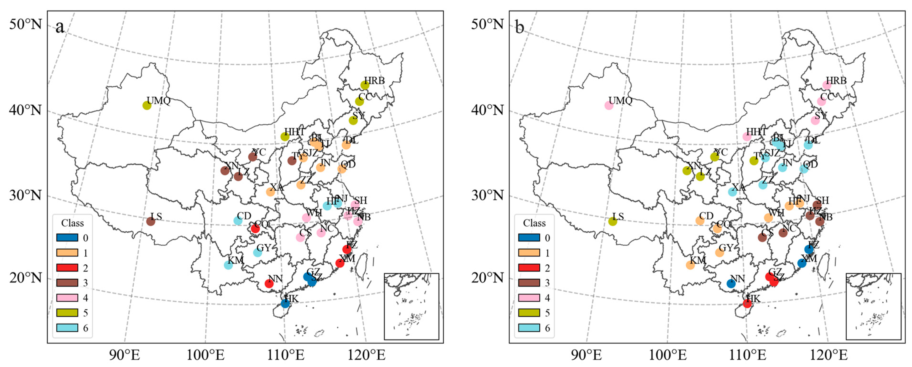
In this section, we further classify the climate using daily mean, maximum, and minimum temperatures, as well as daily precipitation, calculated from hourly data. The results of clustering using k-means and k-medoids methods are shown in Figure 7, while the results based on hierarchical clustering are illustrated in Figure 8.
Comparing the results of k-means (Figure 7a) and k-medoids (Figure 7b) clustering, four out of the seven categories are the same, including three classifications in northern China and one classification comprising Guangzhou, Shenzhen, and Haikou in the south. Discrepancies in the remaining three categories, located in middle and southern China, are attributed to the cities of Chongqing and Wuhan. Overall, the climate classifications by the two non-hierarchical clustering methods based on daily meteorological sequences are largely similar.
However, when comparing non-hierarchical clustering using daily value sequences (Figure 7) and hourly sequences (Figure 3), none of the classification categories are identical. Compared with the non-hierarchical clustering results using hourly data (Figure 3), the results obtained from daily meteorological sequences (Figure 7) may not be entirely “coherent” in terms of geographical locations. For example, based on daily value sequences, the two non-hierarchical clustering methods group the northwestern cities of Urumqi and Hohhot with the northeastern cities of Harbin, Changchun, and Shenyang into one category (Figure 7), and the k-means method groups Chongqing, Nanning, Fuzhou, and Xiamen into one category (Figure 7a). However, from a geographical perspective, the locations of Chongqing, Nanning, Fuzhou, and Xiamen are not contiguous.
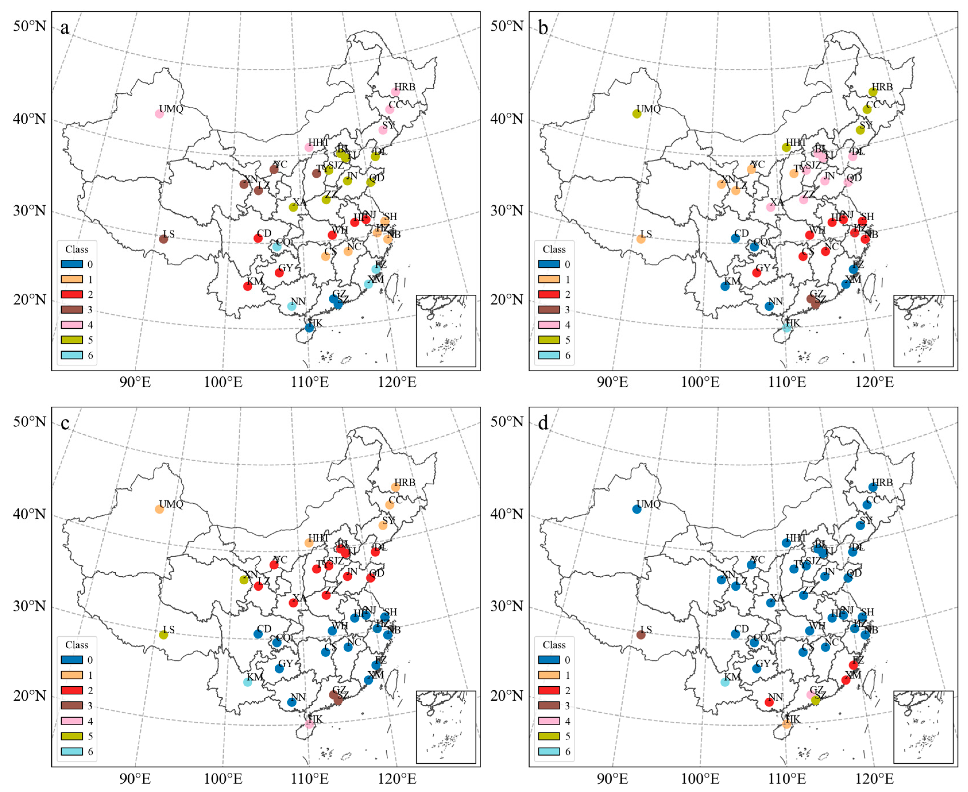
The results of hierarchical clustering are presented in Figure 8, and these four clustering methods yield differing outcomes. While the ward (Figure 8a) and complete (Figure 8b) methods have three identical categories for stations in northern China, the classification for stations in southern China differs. The other two clustering methods, average (Figure 8c) and single (Figure 8d), exhibit unbalanced clustering results, with some clusters being too large and others too small. This suggests that we should try to minimize the use of average and single hierarchical clustering methods.
Comparing Figure 3 with Figure 7, and comparing Figure 5 with Figure 8, it can be seen that the temporal resolution of the input data and the clustering methods significantly impact the climate classification results. In order to objectively assess the climate classification effects of different input data and clustering methods, we will conduct a clustering evaluation in the next section.

3.6. Clustering Evaluation

Previous analyses show that the average and single hierarchical clustering methods often lead to unbalanced clustering results, suggesting a need to minimize their application. In addition, the Köppen–Geiger climate classification is based on the meteorological variables of temperatures and precipitation [2]. Subsequently, this section employs the silhouette coefficient and Calinski–Harabasz indices to assess four types of input data using the four clustering methods of k-means, k-medoids, as well as the ward and complete hierarchical clustering methods. The four inputs include: hourly original sequences of T2, PRE, and RH (hourly data with RH); hourly original sequences of T2 and PRE (hourly data without RH); daily sequences of T2, PRE, and RH (daily data with RH); and daily sequences of T2 and PRE (daily data without RH). The silhouette coefficient and Calinski–Harabasz indices are computed separately for the clustering results obtained. The clustering evaluation indices for each method are illustrated in Figure 9.
The two indices, the silhouette coefficient and the Calinski–Harabasz, both indicate that larger values correspond to better clustering results [43]. In Figure 9a, the input data, comprising hourly sequences with RH, consistently achieve the highest silhouette coefficient across k-means, k-medoids, as well as the ward and complete hierarchical clustering methods. The silhouette coefficient for the hourly sequences with RH surpasses that for the hourly sequences without RH, and similarly, the silhouette coefficient for daily sequences with RH is greater than that for daily sequences without RH. Notably, the k-means and k-medoids algorithms yield the highest silhouette coefficient (0.177) among all clustering results when processing the hourly sequences with RH. Additionally, when processing the hourly sequences without RH, the k-medoids method slightly outperforms k-means, followed by the ward method and complete method.
In Figure 9b, the results for the Calinski–Harabasz index align with the conclusions drawn from the silhouette coefficient. The input data of hourly sequences with RH obtains the highest Calinski–Harabasz index across all clustering algorithms. The Calinski–Harabasz index for the hourly sequences with RH is higher than that for the hourly sequences without RH, and similarly for the daily sequences with RH. Among all the clustering methods, the k-means and k-medoids algorithms achieve the highest Calinski–Harabasz index (8.516) when processing the hourly sequences with RH.
The evaluation results depicted in Figure 9 show that incorporating the meteorological variable of RH, in addition to T2 and PRE, as a clustering input enhances the clustering results, as evidenced by improved silhouette coefficient and Calinski–Harabasz indices. Moreover, utilizing meteorological inputs with a higher temporal resolution leads to superior clustering outcomes, with clustering based on hourly meteorological inputs outperforming that based on daily inputs. In this study, focused on climate classification for major cities in China, the k-medoids method emerges as the best clustering method, followed by k-means, ward, and complete methods.

4. Conclusions

The changing climate necessitates a comprehensive reassessment of climate classifications using updated meteorological data. This study utilizes hourly observations from 2011 to 2021 to classify the climate in 36 major cities in China. The classification methods include the traditional Köppen–Geiger climate classification method, non-hierarchical clustering of k-means and k-medoids, as well as hierarchical clustering of ward, complete, average, and single methods. The findings are as follows.
Firstly, data-driven clustering methods, particularly k-means and k-medoids, outperform the traditional Köppen–Geiger method in classifying climates, reducing variability within the same class, and assigning cities to more suitable climate groups. Among hierarchical clustering methods, ward and complete methods produce more balanced outcomes compared to average and single methods. The most effective method for climate classification is found to be k-medoids, followed by k-means, ward, and complete methods.
Secondly, by setting the parameter k = 2, k-means, k-medoids, ward, and complete methods effectively identify the climate boundaries between the north and south in China, aligning closely with the traditional geographical division along the Qinling–Huaihe River line. This finding underscores the alignment of data-driven methods with established geographical divisions, while also suggesting potential shifts influenced by climate change.
Thirdly, utilizing hourly meteorological data has improved the accuracy and reliability of climate classifications compared to using daily data, capturing more precise climate variations. Both the silhouette coefficient and Calinski–Harabasz indices confirm that including RH along with T2 and PRE has improved the clustering performance, emphasizing the importance of considering multiple meteorological variables.
In conclusion, this study underscores the advantages of using high-resolution, multi-variable meteorological data and data-driving methods for climate classification. Future research could extend these methodologies to encompass a broader range of meteorological stations, including urban and non-urban stations, across different regions in China, which can provide a more comprehensive understanding of the country’s varied climatic patterns.

Author Contributions

Conceptualization, Q.L. and H.D.; methodology, H.D., Q.L. and L.H.; software, H.D.; validation, H.D., Q.L., L.H. and J.Z.; formal analysis, H.D.; investigation, Q.L. and H.D.; resources, Q.L; data curation, Q.L. and H.D.; writing—original draft preparation, Q.L. and H.D.; writing—review and editing, L.H., J.Z., H.A., R.A. and M.V.; visualization, H.D.; supervision, Q.L.; project administration, Q.L.; funding acquisition, Q.L. All authors have read and agreed to the published version of the manuscript.

Funding

This research was funded by the Shenzhen Municipal Committee of Science and Technology Innovation with Grants of GJHZ20210705141403010 and JCYJ20210324101006016.

Institutional Review Board Statement

Not applicable.

Informed Consent Statement

Not applicable.

Data Availability Statement

The data used for this paper are available from the following repository: https://gitee.com/li_qinglan88/climate-classification-for-major-cities-in-china-using-cluster-analysis (accessed on 16 June 2024).

Conflicts of Interest

The authors declare no conflicts of interest.

References

  1. Yang, L.; Gao, X.; Li, Z.; Jia, D. Intra-Day Solar Irradiation Forecast Using Machine Learning with Satellite Data. Sustain. Energy Grids Netw. 2023, 36, 101212. [Google Scholar] [CrossRef]
  2. Peel, M.C.; Finlayson, B.L.; McMahon, T.A. Updated World Map of the Köppen-Geiger Climate Classification. Hydrol. Earth Syst. Sci. 2007, 11, 1633–1644. [Google Scholar] [CrossRef]
  3. Chen, D.; Chen, H.W. Using the Köppen Classification to Quantify Climate Variation and Change: An Example for 1901–2010. Environ. Dev. 2013, 6, 69–79. [Google Scholar] [CrossRef]
  4. Shi, J.; Yang, L. A Climate Classification of China through K-Nearest-Neighbor and Sparse Subspace Representation. J. Clim. 2020, 33, 243–262. [Google Scholar] [CrossRef]
  5. Stern, H.; de Hoedt, G.; Ernst, J. Objective Classification of Australian Climates. Aust. Meteorol. Mag. 2000, 49, 87–96. [Google Scholar]
  6. Kumar, J.; Mills, R.T.; Hoffman, F.M.; Hargrove, W.W. Parallel K-Means Clustering for Quantitative Ecoregion Delineation Using Large Data Sets. Procedia Comput. Sci. 2011, 4, 1602–1611. [Google Scholar] [CrossRef]
  7. Petrić, M.; Lalić, B.; Pajović, I.; Micev, S.; Đurđević, V.; Petrić, D. Expected Changes of Montenegrin Climate, Impact on the Establishment and Spread of the Asian Tiger Mosquito (Aedes albopictus), and Validation of the Model and Model-Based Field Sampling. Atmosphere 2018, 9, 453. [Google Scholar] [CrossRef]
  8. He, H.; Luo, G.; Cai, P.; Hamdi, R.; Termonia, P.; De Maeyer, P.; Kurban, A.; Li, J. Assessment of Climate Change in Central Asia from 1980 to 2100 Using the Köppen-Geiger Climate Classification. Atmosphere 2021, 12, 123. [Google Scholar] [CrossRef]
  9. Köppen, W. Versuch Einer Klassifikation Der Klimate, Vorzugsweise Nach Ihren Beziehungen Zur Pflanzenwelt. Geogr. Z. 1900, 6, 593–611. [Google Scholar]
  10. Beck, H.E.; Zimmermann, N.E.; McVicar, T.R.; Vergopolan, N.; Berg, A.; Wood, E.F. Present and Future Köppen-Geiger Climate Classification Maps at 1-Km Resolution. Sci. Data 2018, 5, 180214. [Google Scholar] [CrossRef]
  11. Thornthwaite, C.W. Problems in the Classification of Climates. Geogr. Rev. 1943, 33, 233–255. [Google Scholar] [CrossRef]
  12. IPCC Summary For Policymakers. Climate Change 2021: The Physical Science Basis; Masson-Delmotte, V., Zhai, P., Pirani, A., Connors, S.L., Péan, C., Berger, S., Caud, N., Chen, Y., Goldfarb, L., Gomis, M.I., et al., Eds.; Cambridge University Press: Cambridge, UK; New York, NY, USA, 2021; pp. 3–32. ISBN 978-1-00-915789-6. [Google Scholar]
  13. Zhang, X. Newly Compiled Geoliterature; Wenming Publishing House: Shanghai, China, 1908. (In Chinese) [Google Scholar]
  14. Zhang, Q.; Han, L.; Lin, J.; Cheng, Q. North–South Differences in Chinese Agricultural Losses Due to Climate-Change-Influenced Droughts. Theor. Appl. Clim. 2018, 131, 719–732. [Google Scholar] [CrossRef]
  15. Qin, Z.; Zhao, J.; Cheng, W.; Wang, J.; Su, H.; He, Y. Change of subtropical northern boundary in Qinling−Huaihe region in the context of climate change. Adv. Clim. Chang. Res. 2023, 19, 38–48. [Google Scholar] [CrossRef]
  16. He, S.; Hao, C. Analysis on Spatial-Temporal Variation Characteristics of Climate in Qinling-Huaihe Demarcation Zone since 1961. Ecol. Indic. 2024, 158, 111345. [Google Scholar] [CrossRef]
  17. Zscheischler, J.; Mahecha, M.D.; Harmeling, S. Climate Classifications: The Value of Unsupervised Clustering. Procedia Comput. Sci. 2012, 9, 897–906. [Google Scholar] [CrossRef]
  18. Iyigun, C.; Türkeş, M.; Batmaz, İ.; Yozgatligil, C.; Purutçuoğlu, V.; Koç, E.K.; Öztürk, M.Z. Clustering Current Climate Regions of Turkey by Using a Multivariate Statistical Method. Theor. Appl. Clim. 2013, 114, 95–106. [Google Scholar] [CrossRef]
  19. Yao, C.S. A New Method of Cluster Analysis for Numerical Classification of Climate. Theor. Appl. Clim. 1997, 57, 111–118. [Google Scholar] [CrossRef]
  20. Gerstengarbe, F.-W.; Werner, P.C.; Fraedrich, K. Applying Non-Hierarchical Cluster Analysis Algorithms to Climate Classification: Some Problems and Their Solution. Theor. Appl. Clim. 1999, 64, 143–150. [Google Scholar] [CrossRef]
  21. Fovell, R.G.; Fovell, M.-Y.C. Climate Zones of the Conterminous United States Defined Using Cluster Analysis. J. Clim. 1993, 6, 2103–2135. [Google Scholar] [CrossRef]
  22. Sa’adi, Z.; Shahid, S.; Shiru, M.S. Defining Climate Zone of Borneo Based on Cluster Analysis. Theor. Appl. Clim. 2021, 145, 1467–1484. [Google Scholar] [CrossRef]
  23. Mimmack, G.M.; Mason, S.J.; Galpin, J.S. Choice of Distance Matrices in Cluster Analysis: Defining Regions. J. Clim. 2001, 14, 2790–2797. [Google Scholar] [CrossRef]
  24. Zhang, X.; Yan, X. Temporal Change of Climate Zones in China in the Context of Climate Warming. Theor. Appl. Clim. 2014, 115, 167–175. [Google Scholar] [CrossRef]
  25. Kalkstein, L.S.; Tan, G.; Skindlov, J.A. An Evaluation of Three Clustering Procedures for Use in Synoptic Climatological Classification. J. Appl. Meteorol. Climatol. 1987, 26, 717–730. [Google Scholar] [CrossRef]
  26. Netzel, P.; Stepinski, T. On Using a Clustering Approach for Global Climate Classification. J. Clim. 2016, 29, 3387–3401. [Google Scholar] [CrossRef]
  27. Unal, Y.; Kindap, T.; Karaca, M. Redefining the Climate Zones of Turkey Using Cluster Analysis. Int. J. Climatol. 2003, 23, 1045–1055. [Google Scholar] [CrossRef]
  28. Carvalho, M.J.; Melo-Gonçalves, P.; Teixeira, J.C.; Rocha, A. Regionalization of Europe Based on a K-Means Cluster Analysis of the Climate Change of Temperatures and Precipitation. Phys. Chem. Earth Parts A/B/C 2016, 94, 22–28. [Google Scholar] [CrossRef]
  29. Mahlstein, I.; Knutti, R. Regional Climate Change Patterns Identified by Cluster Analysis. Clim. Dyn. 2010, 35, 587–600. [Google Scholar] [CrossRef]
  30. Bai, L.; Song, B.; Yang, L. Developing the New Thermal Climate Zones of China for Building Energy Efficiency Using the Cluster Approach. Atmosphere 2022, 13, 1498. [Google Scholar] [CrossRef]
  31. José-García, A.; Gómez-Flores, W. A Survey of Cluster Validity Indices for Automatic Data Clustering Using Differential Evolution. In Proceedings of the Genetic and Evolutionary Computation Conference; Association for Computing Machinery: New York, NY, USA, 2021; pp. 314–322. [Google Scholar]
  32. Qi, W.; Liu, S.; Zhao, M.; Liu, Z. China’s Different Spatial Patterns of Population Growth Based on the “Hu Line”. J. Geogr. Sci. 2016, 26, 1611–1625. [Google Scholar] [CrossRef]
  33. Shrikant, K.; Gupta, V.; Khandare, A.; Furia, P. A Comparative Study of Clustering Algorithm. In Proceedings of the Intelligent Computing and Networking; Balas, V.E., Semwal, V.B., Khandare, A., Eds.; Springer Nature: Singapore, 2022; pp. 219–235. [Google Scholar]
  34. Ahmed, M.; Seraj, R.; Islam, S.M.S. The K-Means Algorithm: A Comprehensive Survey and Performance Evaluation. Electronics 2020, 9, 1295. [Google Scholar] [CrossRef]
  35. Xu, R.; Wunsch, D. Survey of Clustering Algorithms. IEEE Trans. Neural Netw. 2005, 16, 645–678. [Google Scholar] [CrossRef]
  36. Velmurugan, T.; Santhanam, T. A Survey of Partition Based Clustering Algorithms in Data Mining: An Experimental Approach. Inf. Technol. J. 2011, 10, 478–484. [Google Scholar] [CrossRef]
  37. Arthur, D.; Vassilvitskii, S. K-Means++: The Advantages of Careful Seeding. In Proceedings of the SODA, New Orleans, LA, USA, 7–9 January 2007; Volume 7, pp. 1027–1035. [Google Scholar]
  38. Kaufman, L.; Rousseeuw, P.J. Finding Groups in Data: An Introduction to Cluster Analysis; John Wiley & Sons: Hoboken, NJ, USA, 2009; ISBN 978-0-470-31748-8. [Google Scholar]
  39. Massaro, J.M. Clustering, Single Linkage. In Wiley StatsRef: Statistics Reference Online; John Wiley & Sons, Ltd.: Hoboken, NJ, USA, 2014; ISBN 978-1-118-44511-2. [Google Scholar]
  40. Ward, J.H., Jr. Hierarchical Grouping to Optimize an Objective Function. J. Am. Stat. Assoc. 1963, 58, 236–244. [Google Scholar] [CrossRef]
  41. Lance, G.N.; Williams, W.T. A General Theory of Classificatory Sorting Strategies: 1. Hierarchical Systems. Comput. J. 1967, 9, 373–380. [Google Scholar] [CrossRef]
  42. Aghabozorgi, S.; Seyed Shirkhorshidi, A.; Ying Wah, T. Time-Series Clustering—A Decade Review. Inf. Syst. 2015, 53, 16–38. [Google Scholar] [CrossRef]
  43. Zhou, K.; Yang, S.; Ding, S.; Luo, H. On cluster validation. Syst. Eng.-Theory Pract. 2014, 34, 2417–2431. [Google Scholar]
  44. Tavakoli, N. Seq2Image: Sequence Analysis Using Visualization and Deep Convolutional Neural Network. In Proceedings of the 2020 IEEE 44th Annual Computers, Software, and Applications Conference (COMPSAC), Madrid, Spain, 13–17 July 2020; pp. 1332–1337. [Google Scholar]
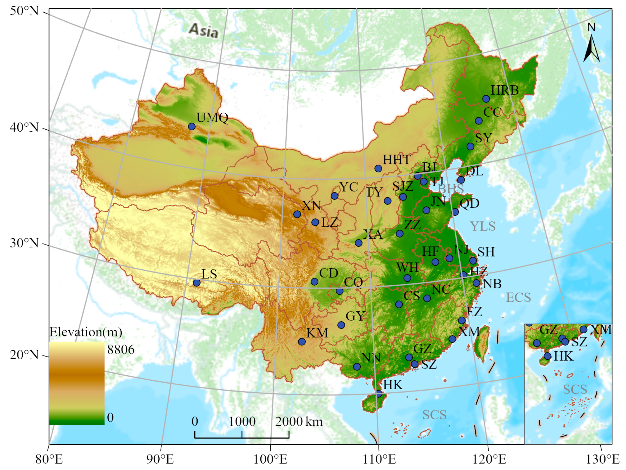
Figure 1. Locations of the 36 basic meteorological stations in the major cities of China. The abbreviations of the stations’ names are shown in Table 1. BHS, YLS, ECS, and SCS refer to Bohai Sea, Yellow Sea, East China Sea, and South China Sea, respectively.
Atmosphere 15 00741 g001
Figure 2. Köppen–Geiger climate classification for the 36 major cities in China.
Atmosphere 15 00741 g002
Figure 3. Climate classification with k = 7 for the 36 stations based on original hourly meteorological observations using (a) k-means and (b) k-medoids clustering methods.
Atmosphere 15 00741 g003
Figure 4. Comparison of Köppen–Geiger climate classification (left column) and k-means clustering (right column) based on climate variables of annual average temperature ( T m e a n ), relative humidity ( R H m e a n ), average annual maximum and minimum temperatures ( T m a x and T m i n ), relative humidity ( R H m a x and R H m i n ), and annual accumulated precipitation ( P R E ). The box plots illustrate the climate variable values of stations within each category, with the values to the right of each sub-plot indicating the maximum difference in climate variables between stations within the same category.
Atmosphere 15 00741 g004
Figure 5. Climate classification with k = 7 for the 36 stations based on original hourly meteorological observations by four hierarchical clustering methods: (a) ward, (b) complete, (c) average, and (d) single.
Atmosphere 15 00741 g005
Figure 6. (a) Traditional division of China into northern and southern regions along the Qinling–Huaihe River line; climate classification with k = 2 for the 36 stations based on original hourly meteorological observations by two non-hierarchical clustering methods and four hierarchical clustering methods: (b) k-means, (c) k-medoids, (d) ward, (e) complete, (f) average, and (g) single.
Atmosphere 15 00741 g006
Figure 7. Climate classification with k = 7 for the 36 stations based on daily meteorological observations using (a) k-means and (b) k-medoids clustering methods.
Atmosphere 15 00741 g007
Figure 8. Climate classification with k = 7 for the 36 stations based on daily meteorological sequences by four hierarchical clustering methods: (a) ward, (b) complete, (c) average, and (d) single.
Atmosphere 15 00741 g008
Figure 9. Climate clustering evaluations based on (a) silhouette coefficient and (b) Calinski–Harabasz.
Atmosphere 15 00741 g009
Table 1. Detailed information for national basic meteorological stations in major cities (arranged in descending order of latitude).
CityAbbreviationProvinceLongitude (°E)Latitude (°N)Altitude (m)
HarbinHRBHeilongjiang126.845.8117.7
ChangchunCCJilin125.243.9237.5
UrumqiUMQXinjiang87.743.8925
ShenyangSYLiaoning123.541.749.5
HohhotHHTInner Mongolia111.740.81154.4
BeijingBJBeijing116.539.832.5
TianjinTJTianjin117.139.24.6
DalianDLLiaoning121.638.992.5
YinchuanYCNingxia106.238.51111.6
ShijiazhuangSJZHebei114.438.081
TaiyuanTYShanxi112.637.8777.3
XiningXNQinghai101.836.72296
JinanJNShandong117.036.6171.2
QingdaoQDShandong120.336.175.3
LanzhouLZGansu103.936.11517.2
ZhengzhouZZHenan113.734.7111.6
XianXAShaanxi108.934.1425.5
NanjingNJJiangsu118.931.936.4
HefeiHFAnhui117.331.828.2
ShanghaiSHShanghai121.531.46.7
WuhanWHHubei114.130.624.4
ChengduCDSichuan103.930.6495.8
HangzhouHZZhejiang120.230.242.6
LhasaLSXizang91.129.73648.9
ChongqingCQChongqing106.529.6259.6
NingboNBZhejiang121.429.340.4
NanchangNCJiangxi116.028.632.9
ChangshaCSHunan112.928.269.2
GuiyangGYGuizhou106.726.61224.9
FuzhouFZFujian119.326.184.8
KunmingKMYunnan102.725.01889.1
XiamenXMFujian118.124.5140.6
GuangzhouGZGuangdong113.523.271.5
NanningNNGuangxi108.222.6122.6
ShenzhenSZGuangdong114.022.563.9
HaikouHKHainan110.320.064.7
Disclaimer/Publisher’s Note: The statements, opinions and data contained in all publications are solely those of the individual author(s) and contributor(s) and not of MDPI and/or the editor(s). MDPI and/or the editor(s) disclaim responsibility for any injury to people or property resulting from any ideas, methods, instructions or products referred to in the content.