Marine Stratus—A Boundary-Layer Model

Abstract

A relatively simple 1D RANS model of the time evolution of the planetary boundary layer is extended to include water vapor and cloud droplets plus transfers between them. Radiative fluxes and flux divergence are also included. An underlying ocean surface is treated as a source of water vapor and as a sink for cloud or fog droplets. With a constant sea surface temperature and a steady wind, initially dry or relatively dry air will moisten, starting at the surface. Turbulent boundary layer mixing will then lead towards a layer with a well-mixed potential temperature (and so temperature decreasing with height) and well-mixed water vapor mixing ratio. As a result, the air will, sooner or later, become saturated at some level, and a stratus cloud will form.

1. Introduction

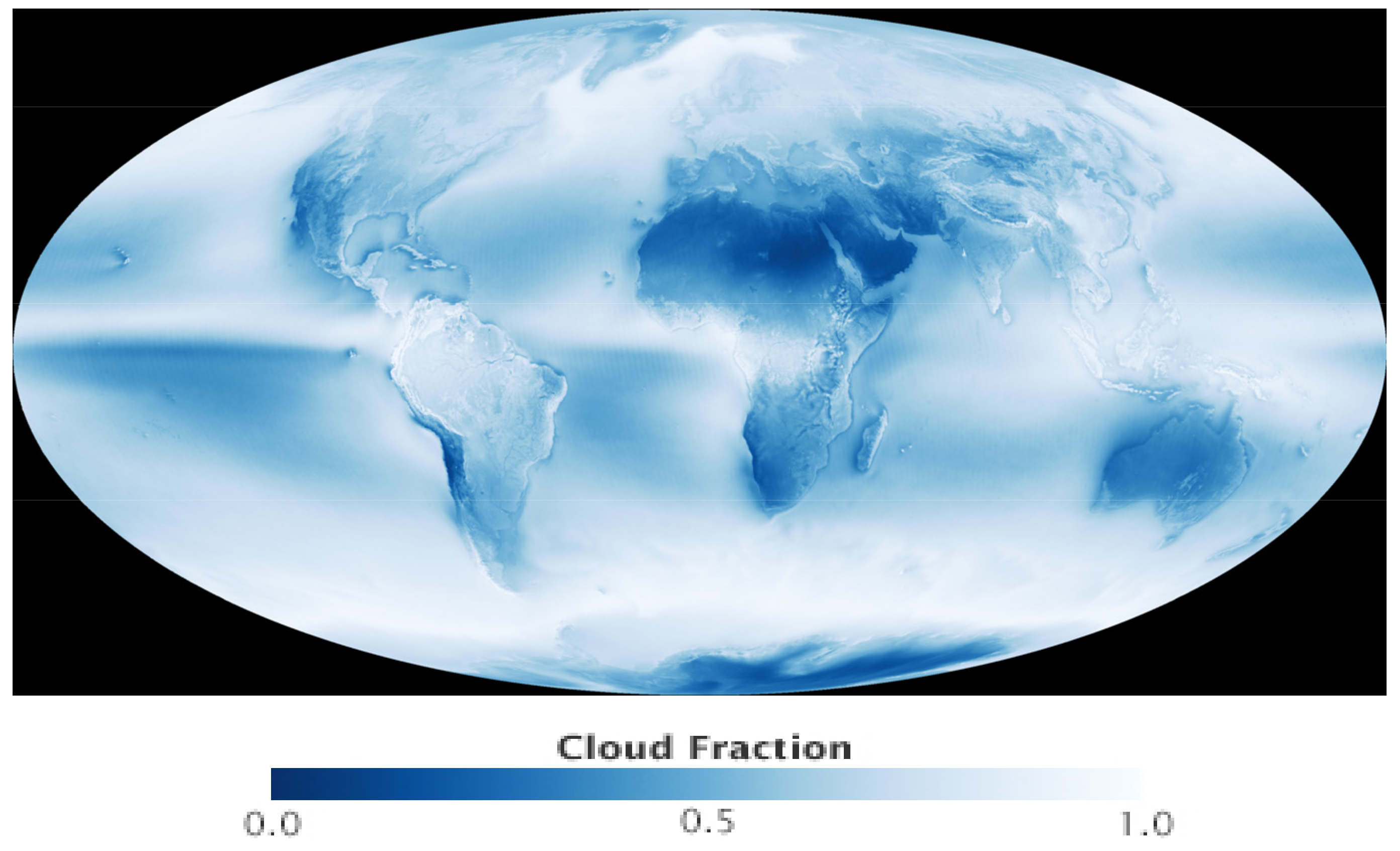
It is clear from Figure 1 that cloud cover is high over mid-latitude ocean surfaces. In collaboration with the Fatima [1] project, my group at York University has been studying and forecasting fog occurrence over the Canadian, coastal N. Atlantic, and over the Yellow Sea near Korea. Our early studies [2,3] with the forecast model, WRF, introduced the idea that the ocean water surface should be a sink for cloud droplets as well as a source for water vapor. In parallel with our WRF modeling, we have developed a separate boundary-layer cloud model.

It is important to stress that the model used here is a relatively simple “toy” model that we are using to explore processes involved in boundary-layer clouds and fog. While others are using 3D high resolution, large eddy simulation models, there is a lot that can be learned from simpler Reynolds-Averaged Navier–Stokes equation (RANS) models and idealized one dimensional situations with assumed horizontal homogeneity. In my group, we also use the Weather Research and Forecasting (WRF) model in both Single Column and 3D forecast modes. Within WRF, just the microphysics module (mp_thompson) has 5470 lines of code and tracking down exactly how things work is not easy! Warm clouds are easier than cold ones, and we also simplify vapor–droplet transitions. These are assumed to occur instantaneously, and we do not have droplet–drizzle–rain transitions—it is a simple model.

In a steady, well-mixed turbulent boundary layer above a water surface, potential temperature (Θ) and water vapor mixing ratio (Q) should, over time, become equal to surface values. The atmospheric boundary layer over the ocean is often capped by stable stratification above 1–2 km, and winds can be strong (of order 20 ms⁻¹). Sample profiles from Sable Island (WSA) are shown in Figure 2. In this case, we see that clouds would have been present from about 500–1250 m with a stable layer at the top. Note that, sadly, the Sable Island radiosonde program ended in 2019 [4].

With potential temperature, Θ(z) ≈ Θ(0), and unsaturated air with the dry adiabatic lapse rate, Γ (= 9.8 K/km), we might expect T(z) ≈ T(0) − Γz, and as a result, the saturation vapor pressure and saturation mixing ratio will decrease with z. In the plots above, the lapse rate is lower (~4 K/km), but the upward mixing of water vapor would still lead to condensation at some level. Since we are assuming saturation at the water surface, we might expect this to start as a surface-based cloud, but the water vapor is mixing upwards, and clouds will initially form higher up. There may be close to 100% relative humidity (RH) in the lower layers of the boundary layer, but the liquid water mixing ratio (QL) is assumed to be 0 at z = 0, and any liquid water would be diffused towards the surface. Katata [5,6] used similar ideas about droplet deposition over vegetation and forests.

Garratt’s (1992) text on the atmospheric boundary layer [7] includes a chapter on the cloud-topped boundary layer or CTBL. It notes that, “The presence of clouds leads to considerable complications compared to a dry ABL (Atmospheric Boundary Layer) because of the important role played by radiative fluxes and phase changes.” There is an excellent discussion of properties and good examples of observations, but Garratt also includes the statement that “relatively few modelling studies have been made on the CTBL”. However, clouds within the boundary layer include fog, and the paper by Fisher and Caplan in 1963 [8] covers both fog and stratus clouds. They develop a preliminary 1D turbulent diffusion model with water vapor and cloud liquid water included. They note the potential significance of radiational cooling but it was not included in their model. In their conclusions, they stress the need for field measurements on the vertical profiles of cloud liquid water content. Some have been made [9], but more are still needed 60 years after their work.

Chapter 7 of Cotton and Anthes’s 1989 book Storm and Cloud Dynamics [10] discusses marine fog and, in particular, the OLW model [11] from 1978. The OLW paper includes predictions of stratus clouds and fogs caused by stratus lowering as well as advective-radiative fogs. It is a RANS model and uses second-order closure, in comparison to our simple model with 1.5-order closure. Radiative flux divergence is included, and vapor–liquid droplet transfers are present within a model with total water and a “conserved” potential temperature (θ_s) as the moisture-related variables. Lower boundary conditions appear to be based on mean surface values of total water mixing ratio and virtual potential temperature (OLW p 305), but it is not clear how liquid water droplets interact with the water surface. Our model will assume that they collide and coalesce so that the water surface is a sink for liquid water in the air (QL(0) = 0). Figure 3 of the OLW paper shows maximum values of QL at the surface in a warm surface fog situation (cold air advected over warm water). Our model would remove those surface droplets by coalescence with the underlying water surface.

There have been other model studies of fog and stratus clouds over water and land surfaces since then, including with NWP models, some single-column versions [12], large eddy simulations [13], and comparisons of both with observations. Work by Koraĉin et al. [14], based on the Lagrangian advection of a 1D model, has similar features to our model described below, although details (see [15,16]) are different. Koraĉin et al. include a large-scale subsidence term, which they see as an important factor in fog caused by stratus lowering. In the coastal California context, they state, “Although the positive fluxes of sensible and latent heat at the air–sea interface are the factors that govern the onset of fog, sensitivity studies with the one-dimensional model indicate that these sensible and latent heat fluxes are of secondary importance as compared to subsidence and cloud-top cooling”. In parallel work on advection fog over cooling surfaces, we can form fog without subsidence.

These earlier papers have generally focused on simulating particular cases, and I am not aware of any high-resolution but simple PBL models presenting the basic situations over ocean water surfaces that we will study here.

2. A 1D PBL Model

Starting from the 1D PBL model (WT) developed with Wensong Weng [17], we can add water vapor and liquid water and allow for transfers between them. We have also added radiative fluxes. In an idealized, horizontally homogeneous ABL and in the absence of radiative flux divergence and moisture, the WT Reynolds-averaged equations (RANS) describing the dynamics of the ABL can be written as shown below. In these equations, upper case symbols, $\mathit{U}$, $V$, $\theta$, etc., represent ensemble or Reynolds-averaged quantities. We assume that W = 0. Lower case, $u$, $v$, $w$, $\theta$, etc., are turbulent fluctuations, and <…> represents an ensemble average. Technically, this is over many realizations of the flow, but in this horizontally homogeneous flow situation, it can be a horizontal average at fixed z and t.

$$\frac{\partial \mathit{U}}{\partial t}=f\left(V-V_g\right)-\frac{\partial <uw>}{\partial z}, \frac{\partial V}{\partial t}=f\left({\mathit{U}}_g-\mathit{U}\right)-\frac{\partial <vw>}{\partial z},$$

(1)

$$\frac{\partial \Theta }{\partial t}=-\frac{\partial <w\theta >}{\partial z}+(RFDIV+LHT)/{(\rho c}_p)$$

(2)

$$\frac{\partial E}{\partial t}=P_s+P_b-\epsilon -\frac{\partial <we>}{\partial z}$$

(3)

Here, RFDIV is radiative flux divergence and LHT is a rate of latent heat release, or demand if negative. These are per unit mass of air. The specific heat of dry air at constant pressure, c_pa, starts as 1005 Jkg⁻¹K⁻¹ but includes adjustments for temperature, and c_p is for moist air accounting for mixing ratios and specific heats of water vapor and liquid water.

c_p = (c_pa(T) + Qc_pv + QLc_l)/M, in J kg⁻¹ K⁻¹

(4)

where the total mass of a volume containing 1 kg of dry air, as a mixing ratio, is

M = 1.0 + Q + QL = constant; with Q and QL ≥ 0

(5)

To these equations, we add conservation equations for water vapor, Q and liquid water, QL mixing ratios, defined in the atmospheric way as mass per unit mass of dry air. These are

$$\frac{\partial Q}{\partial t}=-\frac{\partial <wq>}{\partial z}-\mathsf{\Delta }Q,$$

(6)

$$\mathrm{a}\mathrm{n}\mathrm{d}\hspace{1em}\hspace{1em}\hspace{1em}\frac{\partial QL}{\partial t}=-\frac{\partial <wql>}{\partial z}-\frac{\partial {(W}_{s}QL)}{\partial z}+\mathsf{\Delta }Q.$$

(7)

Here ΔQ is the rate at which water vapor is condensing into, or evaporating from, cloud droplets. It is dependent on the saturation mixing ratio QSAT (T) and computed at each time step in a subroutine which is called “Adjust”. The latent heat added or subtracted in Equation (2), LHT is simply LΔQ, where L is the latent heat of vaporization (2466 J/g at 288 K, but temperature variations are included). W_s is the gravitational settling velocity of the droplets that are formed. Turbulent fluxes are represented by

$$\begin{gathered} -<uw>=K_m\frac{\partial \mathit{U}}{\partial z}, -<vw>=K_m\frac{\partial V}{\partial z}, -<w\theta >=K_h\frac{\partial \Theta }{\partial z} \\ -<wq>=K_q\frac{\partial Q}{\partial z}, -<wql>=K_{ql}\frac{\partial QL}{\partial z}. \end{gathered}$$

(8)

where the eddy diffusivities, K_m, K_h, etc., could differ. In addition, we use an equation for turbulent kinetic energy per unit mass (TKE, E = 0.5 [<u²> + <v²> + <w²>]),

$$\frac{\partial E}{\partial t}=P_s+P_b+\frac{\partial }{\partial z}\left(K_m\frac{\partial E}{\partial z}\right)-\epsilon .$$

(9)

Here P_s and P_b are shear and buoyancy production terms, and ε is the rate of viscous dissipation, details in WT. The eddy diffusivities in this basic E-l, 1.5 order closure are

$$K_m=l_m{\left(\alpha E\right)}^{1/2}, K_h=\frac{K_m}{Pr}, and \frac{1}{l_m}=\frac{{\varphi }_m}{\kappa (z+z_0)}+\frac{1}{l_0}$$

(10)

Again, more details are in WT, but calculations here use α = 0.25, and a Prandtl number, Pr = 1.0. We use the same z₀ for all quantities and ϕ_m is a function of z/L_o where L_o is the Obukhov length, based on local shear stress and heat flux values. In neutral stratification, L_o is infinite and ϕ_m = 1.

Lower boundary conditions on the water surface are U = 0, $\Theta$ = T_surf, the surface water temperature, Q = QSAT (T_surf) and QL = 0. The surface can thus be a source of water vapor but is assumed to be a sink for cloud droplets as they collide and coalesce. Fluxes of momentum, heat, water vapor and liquid water evolve as a part of the solution and depend on the assumed roughness lengths. These can differ, z_0m, z_0h, etc., but are presently all set as z₀ = 0.001 m.

Water droplets can be significant absorbers and emitters of long-wave radiation. For solar radiation, it is sometimes argued that cloud and fog droplets scatter rather than absorb solar radiation and the direct impact may be small. A layer of stratus cloud will, however, significantly reduce downwelling irradiance at the surface, and not all of the down welling energy is backscattered. One website, https://www.foxweather.com/learn/does-fog-really-burn-off-dispelling-the-myth-of-combustible-clouds (accessed on 13 February 2024) states “People commonly refer to the dissipation of fog as ‘burning off’ but the reality is much less exciting”. Fog will forward scatter much of the solar radiation and, over land, will raise the surface and near-surface air temperatures, causing fog to dissipate. Solar radiation will heat up the upper layers of the ocean, but the increase in sea surface temperature is far less than for land surface temperatures, and, over water, the absorption of solar radiation by cloud and fog droplets may be more relevant. There appears to be limited information on the absorption of solar radiation by cloud droplets [18].

To determine the radiative flux divergence, we need to model the four components of irradiance: RFU and RFD for long waves and SFD and SFU for solar radiation. All may be subject to absorption and there will be emission of long-wave radiation by cloud droplets. There will also be absorption and long-wave emissions by the air but for now, although included in the equations, these will be considered as small background effects compared with the local impact of cloud droplets. We also ignore backscattering and use a simple 2-stream (upwelling and downwelling) approach. With air density ρ_a, and using mass absorption coefficients (k_a, k_w, k_sa, k_sw), ignoring backscattering, and with σ as the Stefan–Boltzmann constant, we can write the transfer equations for irradiance as,

$$\frac{\partial RFU}{\partial z}=\left(-RFU+\epsilon \sigma T^4\right)\left(QL{k}_w+k_a\right){\rho }_a,\hspace{1em}\hspace{1em}\frac{\partial RFD}{\partial z}=\left(RFD-\epsilon \sigma T^4\right)(QL{k}_w+k_a){\rho }_a$$

(11)

$$\frac{\partial SFU}{\partial z}=-SFU\left(QL{k}_{sw}+k_{sa}\right){\rho }_a,\hspace{1em}\hspace{1em}\frac{\partial SFD}{\partial z}=SFD\left(QL{k}_{sw}+k_{sa}\right){\rho }_a$$

(12)

Here ρ_a is dry air density. Initially, we neglect clear air absorption (k_a, k_sa = 0), set the emissivity, ε = 1, and focus on absorption coefficients for cloud droplets (k_w, k_sw) with units of m²kg⁻¹. A serious omission is the back scattering and multiple scattering of downwelling solar radiation (SFD) and the contribution to SFU. A more careful treatment of solar radiation is planned for future work.

Boundary conditions are needed on upwelling radiant fluxes at the surface and downwelling fluxes at the model top. These are specified in Section 3.3, based on black body RFU at the water surface and a relatively low albedo (0.05 in cases here) for solar irradiance. At the top boundary (300 m in this case), we specify a typical, clear sky value for RFD (200 Wm⁻² here) and must specify SFD. In realistic simulations, this will have a strong diurnal cycle, but in the test case considered in Section 3.3, we simply set SFD = 250 Wm⁻² and hold it constant.

The heating term added to Equation (2) is

$$RFDIV=\frac{\partial }{\partial z}(RFD+SFD-RFU-SFU).$$

(13)

Our microphysics assumes that condensation occurs instantaneously if the mixing ratio, Q > QSAT(T), the saturation value at air temperature, T. Then Q instantly reduces towards that saturation value with the excess becoming liquid water, QL. This releases latent heat, raises T, and modifies QSAT so that some iteration is needed. An adjustment is made in the opposite direction when liquid droplets diffuse into a sub-saturated layer. A similar approach was used by Brown and Roach [19], but no details were provided. Both transformations are assumed to take place at constant total pressure and with no external source or sink of heat. Our saturation adjustment involves some iteration and is illustrated in Figure 3. QL is not shown but could be computed via Equation (14) below.

The adjustment is between a non-equilibrium state (Q₁, QL₁, T₁) predicted after a time step (Equations (1)–(7)) with Q₁ ≠ QS₁ to an equilibrium state with Q₂ = QS₂, where QS_i = QS(T_i,P), the saturation mixing ratio. Note that no adjustment is needed (Case 1) if Q₁ < QS₁ and QL₁ = 0, but one is needed (Case 2) if Q₁ > QS₁. In Case 4, we may find Q₁ < QS₁ and QL₁ > 0, and liquid water will evaporate, cooling the air. It may also be possible (Case 3), with Q₁ < QS₁ and QL₁ > 0, to evaporate all the droplets while Q₂ < QS₂. Our approach would then predict QL₂ < 0, and adjustments are made to correct for that. The essential feature of the adjustment is that heat per unit mass of the mass of the material undergoing the adjustment is conserved, i.e.,

H = L₁ Q₁ + Mc_p1 T₁ = L₂ Q₂ + Mc_p2 T₂.

(14)

where c_p1 and c_p2 are the specific heats of the dry air plus water vapor and liquid water in states 1 and 2. M is the total mass (dry air plus water vapor and liquid water) per unit mass of dry air, as in Equation (4). This is a constant during the adjustment. In the cases shown, our desired saturation adjustments correspond to the points of intersection of the solid green and blue lines with the black line corresponding to QS(T). If we use the tangent QS line and set c_p = c_p1 in the H = constant line, as in our initial estimates of state 2, we get the points of intersection of the dashed lines. Additional details are at https://www.yorku.ca/pat/AdjustJan2024.pdf (accessed on 7 May 2024).

3. Results

3.1. Initial States

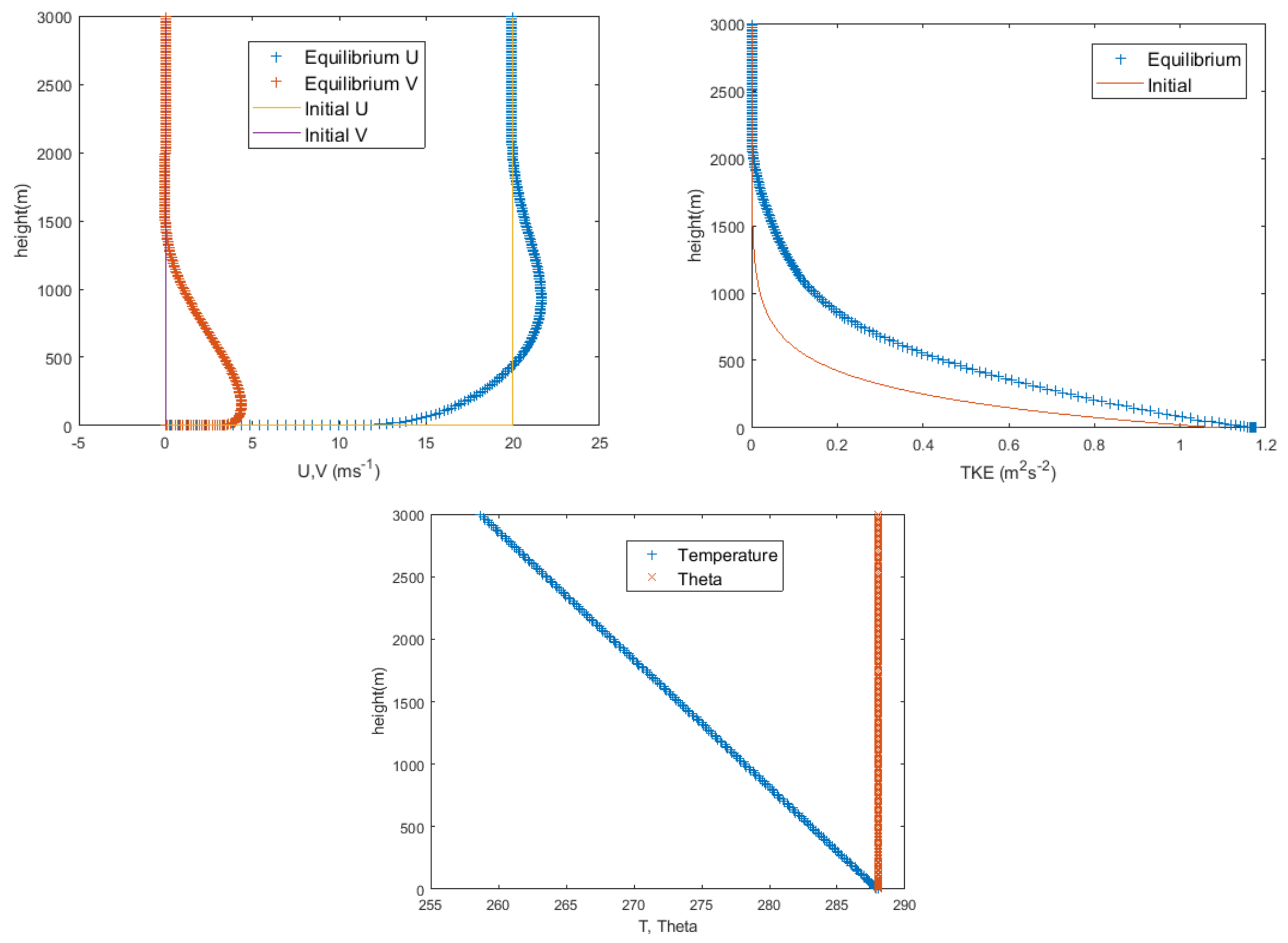
We can run the model with completely dry air, no clouds, and no radiative fluxes to obtain initial profiles. Initial temperature profiles can be for neutral stratification, or we can specify a weak stable stratification. We used either dΘ dz = 0 or 2 K/km and used T_surf = 288 K. We assumed a geostrophic wind U_g= (20, 0) ms⁻¹ with z₀ = 0.001 m and Coriolis parameter, f = 10⁻⁴s⁻¹. Initial TKE was set to a surface value based on the geostrophic drag law and we imposed an exponential decay with height exp(−z/2000 m). As initial conditions for these runs, we simply set U = U_g at all levels. Initial values are not important—we are just seeking an equilibrium steady state. With neutral stratification, we get a typical Ekman spiral profile while Θ is constant and T decreases at the dry adiabatic lapse rate. Results are in Figure 4 and use 241 vertical levels between the surface and a model top at 3 km. The time step used is 2.5 s, and we impose a TKE (E) minimum of 0.00001 m²s⁻².

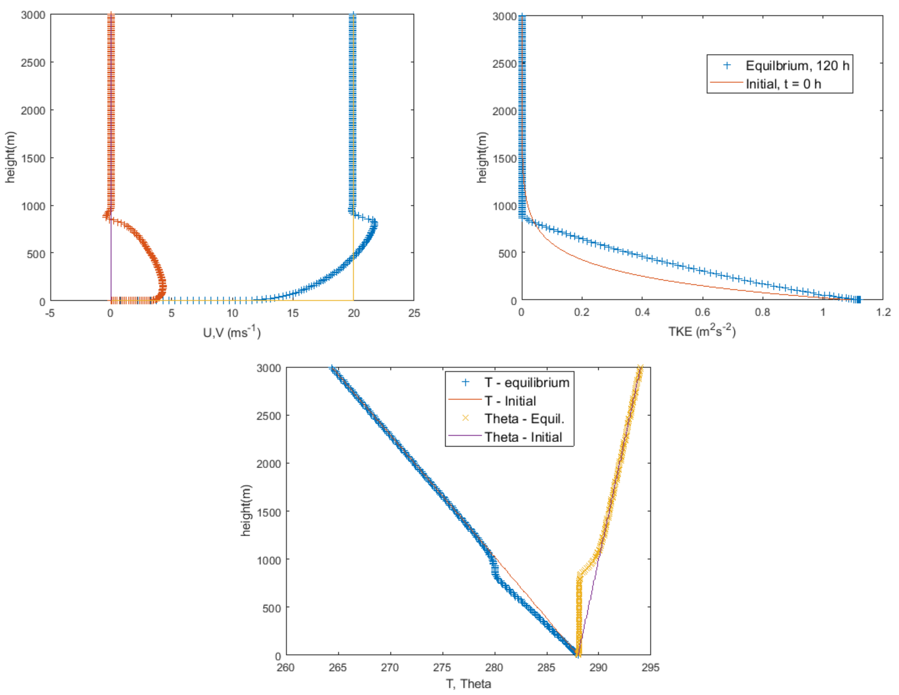
With an initial stable lapse rate, the PBL model will evolve to the state shown in Figure 5. Turbulent mixing will lead to a relatively constant well-mixed potential temperature layer up to about 800 m, in this case, capped by a relatively strong stable layer, while above that, the stratification stays at dΘ/dz = 2 K/km. In that layer near z = 900 m, there can be strong velocity shear and weak inertial oscillations can persist. We will refer to the final profiles as our “2 K/km stable equilibrium”.

3.2. Adding Moisture

We can now restart and continue computations, starting with the U, V, E, Θ stable layer “2K/km equilibrium” profiles discussed in the previous section as initial conditions and now adding moisture effects, and potential condensation. Results after 5 days are shown in Figure 6. Our surface boundary conditions will now include mixing ratios Q = QSAT (T_s), QL = 0 while T_surf is maintained, in this case, at 288 K. We can set initial profiles of Q and QL as we wish, but the extreme case is to have completely dry air with Q = 0 for all z > 0, and QL = 0 for z ≥ 0. Our air column may have been advected from an extremely dry desert out over an ocean.

During the 5 days, starting with RH = 0, water vapor diffuses upwards from the water surface, some condenses and warms the air. In these results, after 5 days, a cloud extends from near the surface (z ~ 30 m) to about z = 944 m, as shown by the RH and QL profiles. Note that there is significant variation in QL within the RH = 1.0 layer, and the QL maximum (about 0.45 g/kg) is far less than that of the Q and QSAT values, which are of order 10 g/kg at the same level. We can allow some gravitational settling of the cloud/fog droplets. In the plots shown, we applied a settling velocity, W_s, of 0.005 ms⁻¹, appropriate to droplets of diameter near 13 μm. Gravitational settling over a day would lead to a descent of 432 m, so it can play a significant role and there will be some sensitivity to the value used.

The droplet formation seems to have occurred through the upper part of the boundary layer, leading to heating by about 1.7 K over the 5 days. This leads to stable stratification in the lower part of the boundary layer and a well-mixed layer above with a top that has risen from about 800 m to 1000 m. Changes in the stratification lead to adjustments of the velocity profiles and weakening of the velocity shear at the boundary-layer top. The TKE profile is also smoothed in these upper layers, and TKE values are reduced because of stable stratification in the lower part of the boundary layer. QSAT profiles are also modified by the temperature change.

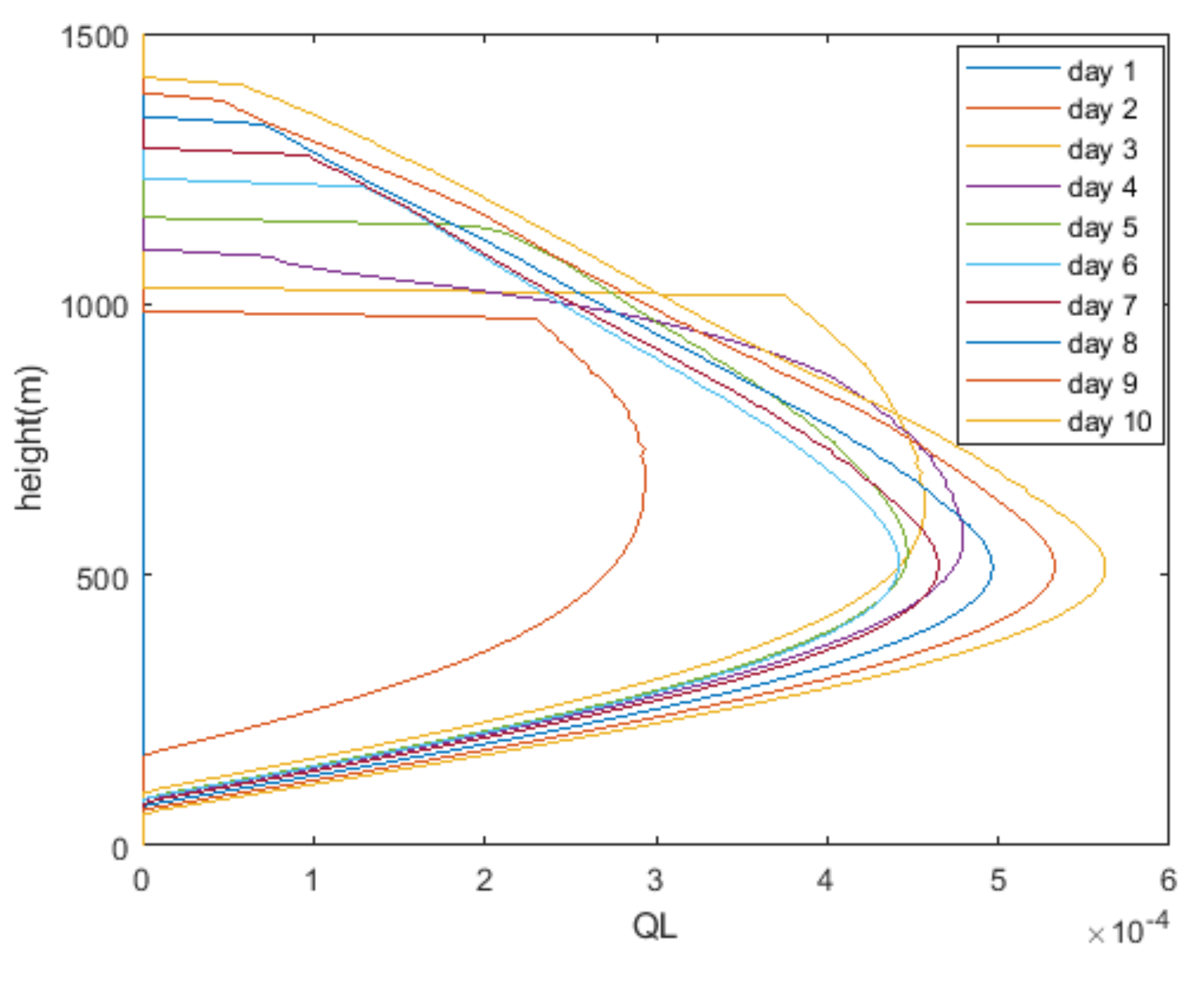
In Figure 7, we show the evolution of the QL profiles over time, and we have extended the computations to 10 days. In this rather extreme case, starting with completely dry air, no cloud has formed after day 1 but appears during day 2, and clouds are present after 30 h in a layer from 500–890m above the surface. The cloud base lowers with time, and the cloud top rises to about 945 m. The drop in QL with height at the cloud top is sharp and stays at about that level for 5 days. Gravitational settling, W_s, does, however, reduce QL at the cloud top, and by day 6, there is a smoother transition to clear air above the cloud (Figure 7). If we start with some moisture present, the cloud forms more quickly and initial cloud water mixing ratios are higher.

If we set Ws = 0, we obtain the results shown in Figure 8, extended to 10 days. The first two days are quite similar to the results with W_s = −0.005 ms⁻¹ shown earlier, but as time moves on, the cloud top continues to rise, and peak QL values slowly increase. There is some sensitivity to the treatment of mixing in stable conditions at the top of the cloud.

3.3. Adding Radiation

Radiative flux absorption, in clear air and in clouds, is a complex process with strong and detailed wavelength and droplet size dependence. We use a simple 2-stream approach for irradiance, upwelling and downwelling, long wave (RFU, RFD), and solar (SFU, SFD). Basically, we use the radiative transfer equation, or Schwarzschild’s equation, integrated over the wavelengths concerned and over the zenith angle, azimuthally averaged, and applied to irradiance. We assume all scattering is forward and that long-wave emissions from cloud droplets produce both upwelling and downwelling long-wave radiation.

One problem with adding radiation effects is finding appropriate grey body irradiance values of the long and short-wave mass absorption cross section coefficients for water droplets, k_w, k_sw. Units will be m²kg⁻¹. Stephens’s paper [18], (his Table 3), leads us to use k_w = 80 m²kg⁻¹ for infrared irradiance. For solar radiation, we initially take k_sw = 40 m²kg⁻¹, but much deeper investigation is needed. Adjustment for solar angle with the time of day would be needed for SFD above, within the cloud, and for k_sw, but for now, we will just set these as constant to illustrate potential solar heating effects. As discussed in Section 2 above, we also need to take into account backscattering within the cloud layer, find appropriate coefficients for that, and find a way to treat diurnal cycles.

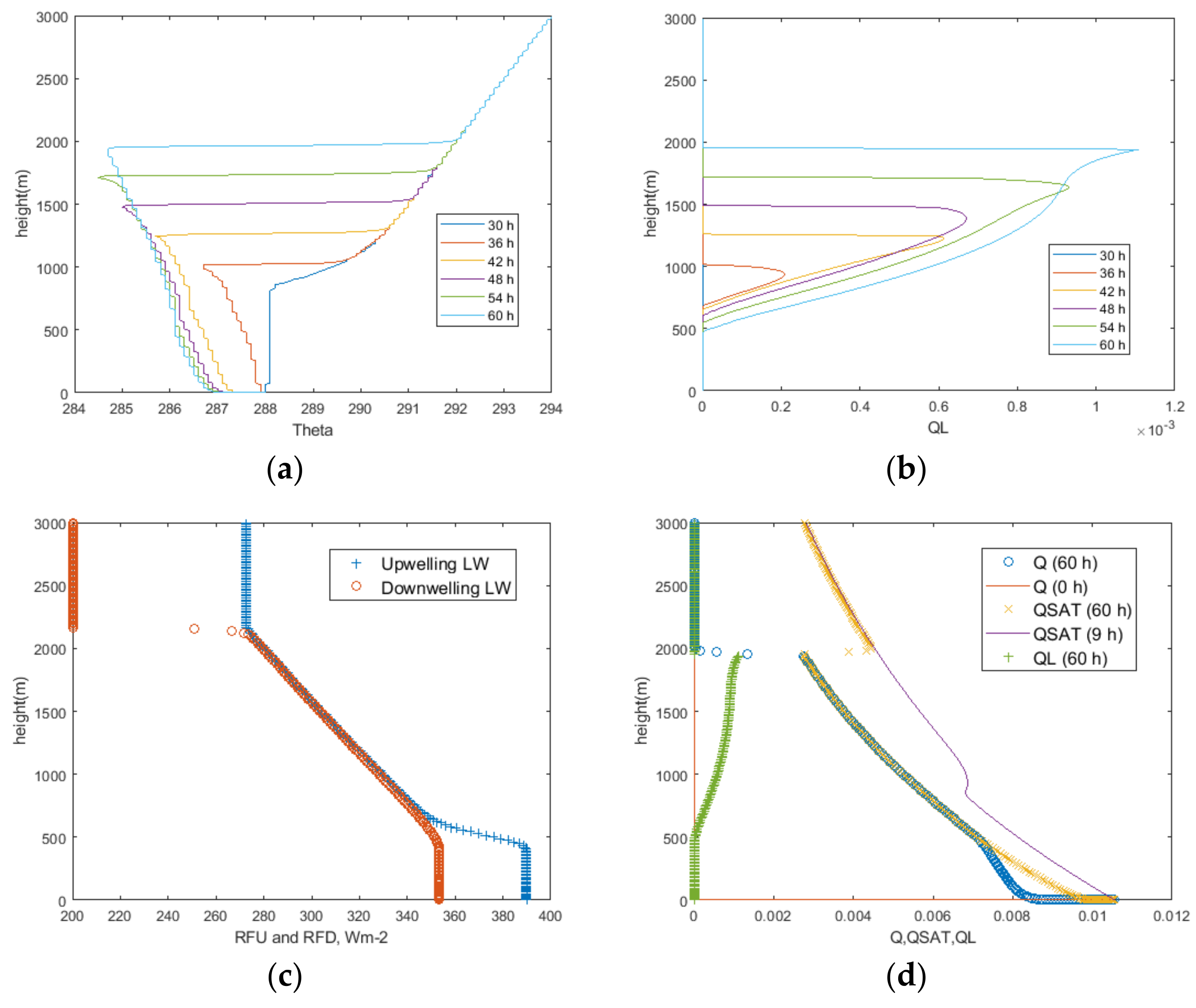
To illustrate the effects of long-wave radiation, we look at a simple sample case with no solar radiation. Other parameters are as in our “2K/km equilibrium” case, which provides our initial conditions. Downwelling long-wave radiation from the air above the model upper boundary (3 km) is set as 200 Wm^−2, and the surface irradiance, at z = 0 m, is the black body value, in this case at 288 K, 390 Wm⁻². Selected results are in Figure 9, extending out to 60 h. Soon after that 60 h point, the model ran into computational problems, probably associated with the extremely strong thermal stability conditions that developed at the cloud top where radiational cooling had dropped the temperature down by about 7 K, as shown in Figure 9a. Results at the 60 h point show upwelling and downwelling long-wave radiation both equal to black body emissions at the cloud water temperature through most of the cloud layer (Figure 9c). Near the cloud base (~500 m), where QL is lower, there is still some unabsorbed radiation from the underlying water surface so that RFU > RFD. Clouds appear at around 30 h, as in the case with no radiation, after which the liquid water content of the cloud increases with time (Figure 9b) and has a maximum near the cloud top where radiational cooling is lowering temperatures, as illustrated in Figure 9a. In Figure 9c, one can see that just at the cloud top level, d(RFD − RFU)/dz will be negative, and, with no solar component, RFDIV is also negative and will cause the cloud top cooling.

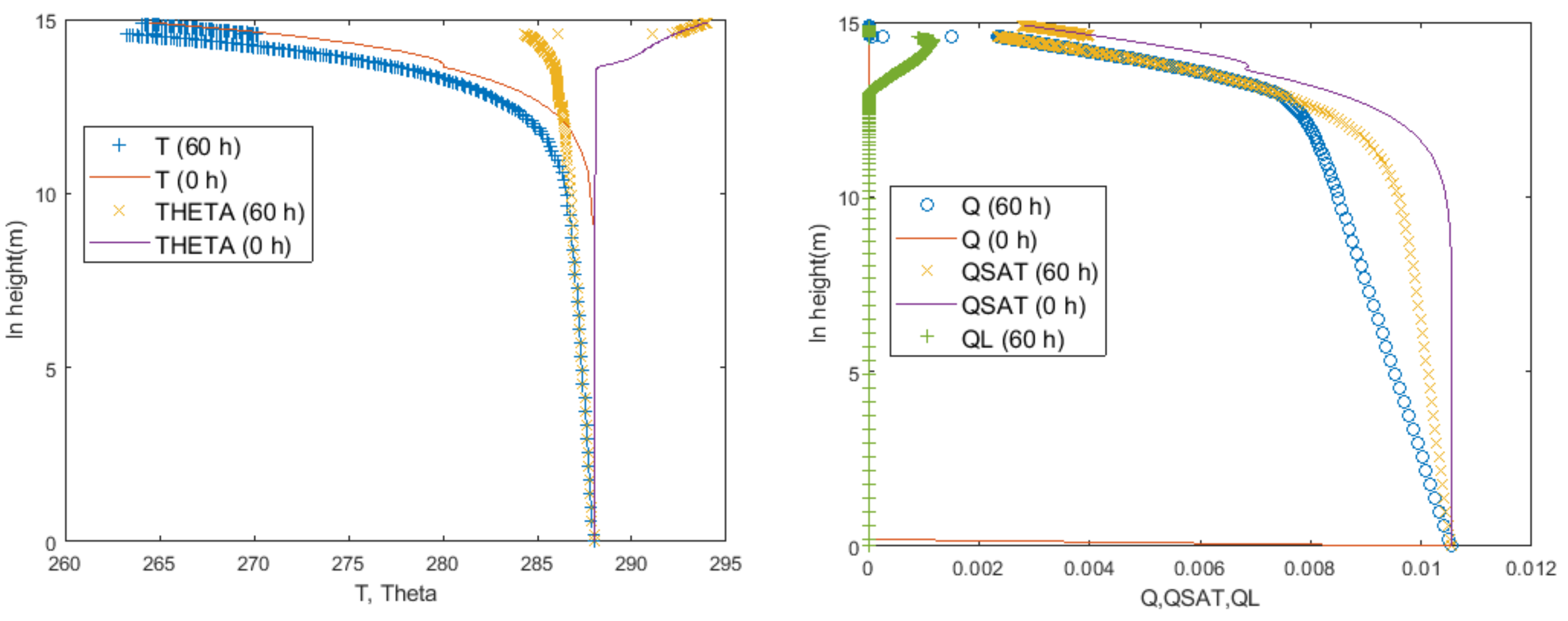
In Figure 9a,d, there are strong variations of T and Q near the surface due to the upward diffusion of heat and water vapor from the surface source towards the cloud layer, where strong radiational cooling and subsequent condensation occur. Plotting temperature and Q profiles against ln z reveals normal log-linear profiles in the sub-cloud layer (Figure 10) while the cloud top data gets rather compressed.

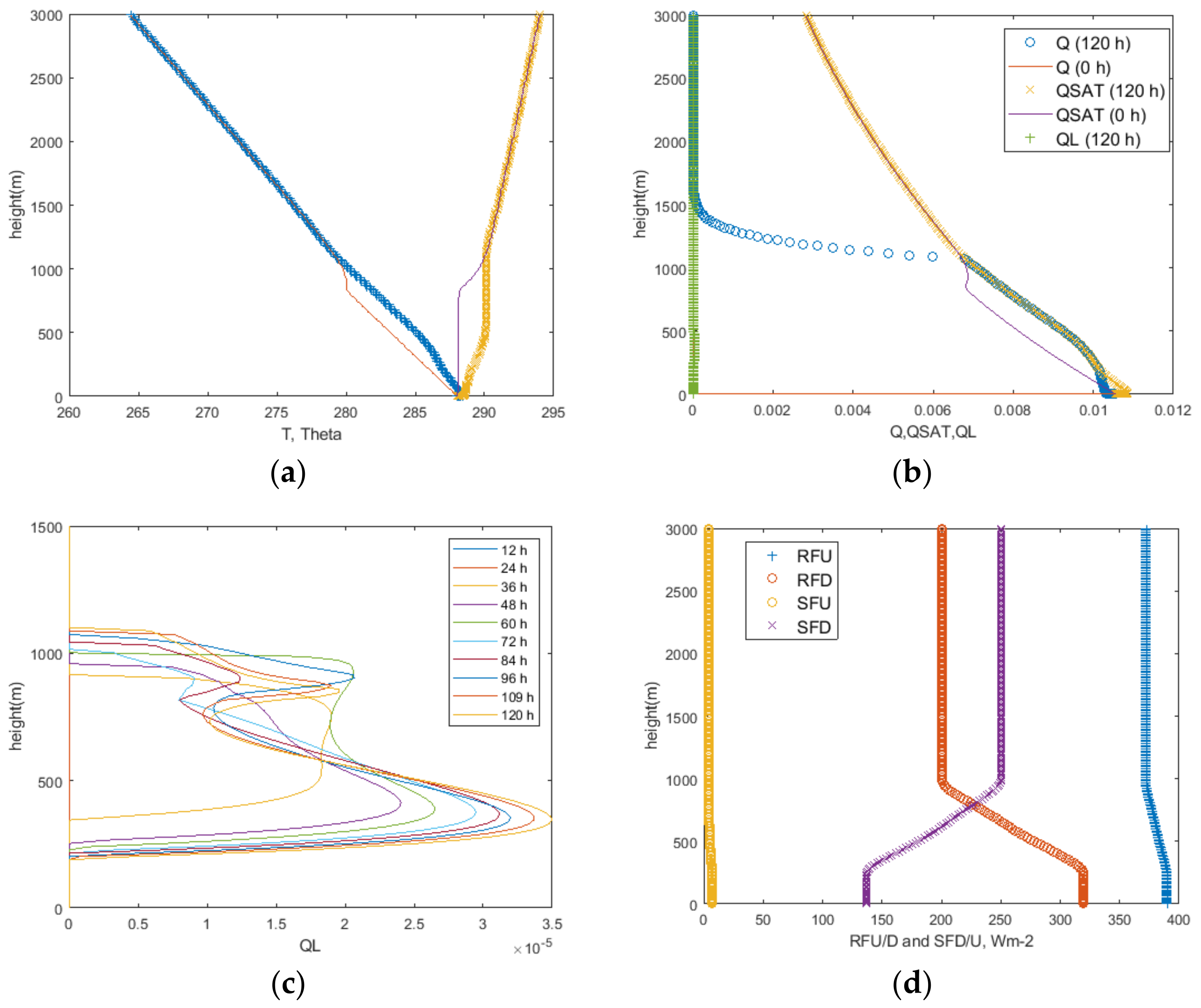
As an idealized exercise, we add solar radiation effects, ignoring diurnal variations and holding incoming solar radiation constant with time. We assume downwelling solar irradiance at the model top of 250 Wm⁻² and hold the absorption coefficient, k_sw = 40 m²kg⁻¹, constant. In this case, a stable situation develops, and Figure 11 shows results after 5 days of development. The boundary layer cloud develops with a base of around 200 m and extends up to ~1100 m. The RH is 1.0 with Q = QSAT (Figure 11b) throughout the cloud layer, but the liquid water content is low and hardly visible in Figure 11b. With a time step of 2.5 s, results in the upper part of the cloud were a little noisy, so we reduced the time step to 0.25 s for Figure 11c (note also a different z scale) above. The maximum QL of around 0.03 g/kg can be compared to 0.5 g/kg in the case with no radiation and ~ 1 g/kg in the long-wave radiation case. At t = 5 days, the four irradiance components are shown in Figure 11d.

In this case, the cloud approaches a relatively steady state in terms of depth after 2 days while QL increases slowly (Figure 11c). If we reduce the solar absorption coefficient, k_sw, to 20 m²kg⁻¹, the QL values are still low (max ~ 0.1 g/kg), and the depth increases steadily with time (~1650 m at t = 5 days), as with no solar radiation.

Typical marine low stratus clouds and fog would have LWC values in the 0.05–0.6 gm⁻³ range, according to Lowmann et al. [20], so g/kg values 0.04–0.5. Our modeled clouds are not precipitating but do have gravitational settling (0.005 ms⁻¹). With no solar radiation, our model QL values (~1 g/kg) are rather high, while our first estimates for QL with solar impacts (~0.03 g/kg) are a little low. However, Isaac et al. [21], in their Figure 12, report groups of fog cases over the Grand Banks, at a height of 69 m, with LWC in ranges of 0.005–0.01 and 0.01–0.05 gm⁻³, and so our QL = 0.03g/kg, LWC = 0.025 gm⁻³, may be realistic while 1.0 g/kg is too high and we may need to assume larger droplet sizes and possibly allow rain to develop.

4. Conclusions

It seems easy to understand why marine clouds occur, but a simple model suggests that the oceans should almost always be cloud covered. Solar radiation, heating, and rainout will allow clear skies at times, along with subsidence. The simple model developed and applied here may give some indication of the processes involved in warm stratus clouds and potentially can be extended to a broader range of conditions.

The essential features are that with moderate or strong winds over an extended water surface, boundary-layer mixing can lead to saturated air at some height above the surface and that this simple model predicts that, even with completely dry air to start with, clouds will form. Oliver et al. [11] suggest that “long-wavelength cooling of the water-vapor-laden air will then lead to condensation somewhere within the layer”. While that may play a role, our argument would be that the development of a layer with well-mixed water vapor and potential temperature is sufficient to generate cloud and that long-wave radiation from cloud droplets is more important than that from water vapor. Long-wave, infra-red radiation from cloud droplets then leads to cloud top cooling and an essentially stable cloud layer. If solar radiation is added, this will modify the cloud profile, but stable cloud layers may still occur.

Further work is needed to better represent solar radiation impacts and to refine other aspects of the model, including appropriate initial humidity conditions to allow more rapid cloud development. The initial aerosol distribution will have a strong impact on the droplet numbers and size distribution. We may need more information than simply QL. A simple model of raindrop formation via collision and coalescence is also needed in order to develop a full life cycle for water evaporating from and eventually returning to the surface as rain.

References

1. Fog and Turbulence Interactions in the Marine Atmosphere. Available online: https://efmlab.nd.edu/research/Fatima/ (accessed on 19 February 2024).
2. Taylor, P.A.; Chen, Z.; Cheng, L.; Afsharian, S.; Weng, W.; Isaac, G.A.; Bullock, T.W.; Chen, Y. Surface deposition of marine fog and its treatment in the Weather Research and Forecasting (WRF) model. Atmos. Chem. Phys. 2021, 21, 14687–14702. [Google Scholar] [CrossRef]
3. Cheng, L.; Chen, Z.; Taylor, P.; Chen, Y.; Isaac, G. Fog over Sable Island. CMOS Bulletin SCMO, 21 June 2021. Available online: https://bulletin.cmos.ca/fog-over-sable-island/ (accessed on 7 May 2024).
4. MSC’s Aerological Program Ends After 75 Years of Service – WSA Sable Island 1944–2019. Available online: https://sableislandinstitute.org/mscs-aerological-program-ends/ (accessed on 7 May 2024).
5. Katata, G.; Kajino, M.; Hiraki, T.; Aikawa, M.; Kobayashi, T.; Nagai, H. A method for simple and accurate estimation of fog deposition in a mountain forest using a meteorological model. J. Geophys. Res. 2011, 116, D20102. [Google Scholar] [CrossRef]
6. Katata, G. Fogwater deposition modeling for terrestrial ecosystems: A review of developments and measurements. J. Geophys. Res. Atmos. 2014, 119, 8137–8159. [Google Scholar] [CrossRef]
7. Garratt, J.R. The Atmospheric Boundary Layer; Cambridge University Press: Cambridge, UK, 1992; 316p. [Google Scholar]
8. Fisher, E.L.; Caplan, P. An experiment in numerical prediction of fog and stratus. J. Atmos. Sci. 1963, 20, 425–437. [Google Scholar] [CrossRef]
9. Ballard, S.; Golding, B.; Smith, R. Mesoscale model experimental forecasts of the Haar of northeast Scotland. Mon. Weather Rev. 1991, 119, 2107–2123. [Google Scholar] [CrossRef]
10. Cotton, W.R.; Anthes, R.A. Storm and Cloud Dynamics; Academic Press: Cambridge, MA, USA, 1989; 880p. [Google Scholar]
11. Oliver, D.A.; Lewellen, W.S.; Williamson, G.G. The Interaction between Turbulent and Radiative Transport in the Development of Fog and Low-Level Stratus. J. Atmos. Sci. 1978, 35, 301–316. [Google Scholar]
12. Bott, A.; Trautmann, T. PAFOG—A new efficient forecast model of radiation fog and low-level stratiform clouds. Atmos. Res. 2002, 64, 191–203. [Google Scholar] [CrossRef]
13. Wainwright, C.; Richter, D.H. Investigating the sensitivity of marine fog to physical and microphysical processes using large-eddy simulation. Bound.-Layer Meteorol. 2021, 181, 473–498. [Google Scholar] [CrossRef]
14. Koračin, D.; Lewis, J.; Thompson, W.T.; Dorman, C.E.; Businger, J.A. Transition of Stratus into Fog along the California Coast: Observations and Modeling. J. Atmos. Sci. 2001, 58, 1714–1731. [Google Scholar] [CrossRef]
15. Koračin, D.; Rogers, D.P. Numerical simulations of the response of the marine atmosphere to ocean forcing. J. Atmos. Sci. 1990, 47, 592–611. [Google Scholar] [CrossRef]
16. Rogers, D.P.; Koračin, D. Radiative transfer and turbulence in the cloud-topped marine atmospheric boundary layer. J. Atmos.Sci. 1992, 49, 1473–1486. [Google Scholar] [CrossRef]
17. Weng, W.; Taylor, P.A. On modelling the 1-D atmospheric boundary layer. Bound.-Layer Meteorol. 2003, 107, 371–400. [Google Scholar] [CrossRef]
18. Stevens, G.L. The Parameterization of Radiation for Numerical Weather Prediction and Climate Models. Mon. Weather Rev. 1984, 112, 826–867. [Google Scholar] [CrossRef]
19. Brown, R.; Roach, W.T. The physics of radiation fog. II. A numerical study. Q. J. R. Meteorol. Soc. 1976, 102, 335–354. [Google Scholar]
20. Lohmann, U.; Lüönd, F.; Mahrt, F. An Introduction to Clouds: From the Microscale to Climate; Cambridge University Press: Cambridge, UK, 2016; 391p. [Google Scholar]
21. Isaac, G.A.; Bullock, T.; Beale, J.; Beale, S. Characterizing and Predicting Marine Fog Offshore Newfoundland and Labrador. Weather Forecast. 2020, 35, 347–365. [Google Scholar] [CrossRef]
Figure 1. Global cloud coverage, from https://earthobservatory.nasa.gov/images/85843/cloudy-earth (accessed on 1 May 2024).
Atmosphere 15 00585 g001
Figure 2. Wind speed, temperature and humidity profiles on a cloudy day over Sable Island, 00Z, 3 July 2019, data from http://weather.uwyo.edu/upperair/sounding.html (accessed on 19 February 2024). Note Θe, ThetaE, is the equivalent potential temperature with the latent heat of water vapor accounted for.
Atmosphere 15 00585 g002
Figure 3. Two saturation adjustment cases (2 and 4) with initial temperature T1 = 288 K plus an illustration of qs(T) and (dashed red line) the linear approximation qsa(T). The solid blue and green lines correspond to H = constant in the two cases. The corresponding dashed lines are first approximations with state 1 values of cp and L and QS varying linearly with T.
Atmosphere 15 00585 g003
Figure 4. Equilibrium planetary boundary layer profiles with neutral stratification and dry air. Initial state had Ug = (20, 0) ms−1 and Θ = 288K for all z. Also note z0 = 0.001m and f = 10−4s−1. Equilibrium profiles are after integration for 5 days.
Atmosphere 15 00585 g004
Figure 5. Equilibrium planetary boundary layer profiles with dry air and stable stratification aloft. Our initial state had Ug = (20, 0) ms−1 and Θ = 288 + 0.002 z K for all z(m). We use the same initial TKE, z0= 0.001 m and f = 10−4s−1, as in Figure 4. Surface temperature (Ts) is maintained at 288 K.
Atmosphere 15 00585 g005
Figure 6. Results after 5 days over a water surface. Thin lines define the initial conditions (equilibrium profiles from Figure 5) and o, +, x symbols are values after 120 h over a water surface with Q(z = 0) = QSAT (288K). Note that temperature and potential temperature are in K, Relative Humidity = 1 is 100% and that mixing ratios, Q, QL, QSAT are in kg/kg.
Atmosphere 15 00585 g006
Figure 7. From the same case as in Figure 6, QL profiles every 6 h, every 12 h snd every 24 h. The first cloud appears after 30 h and a relatively steady profile after 120 h, with a maximum lower than the earlier peak.
Atmosphere 15 00585 g007
Figure 8. Daily QL (kg/kg) profile results with Ws = 0.
Atmosphere 15 00585 g008
Figure 9. Selected results with long-wave radiation, up to 60 h. (a) Potential temperature (K), (b) Liquid water mixing ratio, QL (kg/kg so 10−3 g/kg), (c) Radiative fluxes, long wave, infrared, Wm−2, (d) Mixing ratios, Q, QSAT, QL (kg/kg).
Atmosphere 15 00585 g009
Figure 10. T, Θ (K) and Q, QSAT, QL (kg/kg) results with long-wave radiation after 60 h.
Atmosphere 15 00585 g010
Figure 11. Selected results with long- and short-wave radiation after 120 h. (a) Temperature and potential temperature (K), (b) mixing ratios (kg/kg) (c) Liquid water mixing ratio(kg/kg), (d) radiative fluxes (Wm−2).
Atmosphere 15 00585 g011
Disclaimer/Publisher’s Note: The statements, opinions and data contained in all publications are solely those of the individual author(s) and contributor(s) and not of MDPI and/or the editor(s). MDPI and/or the editor(s) disclaim responsibility for any injury to people or property resulting from any ideas, methods, instructions or products referred to in the content.