Next Article in Journal
State-of-the-Art Low-Cost Air Quality Sensors, Assemblies, Calibration and Evaluation for Respiration-Associated Diseases: A Systematic Review
Next Article in Special Issue
Correction: Taylor et al. A Statistical Forecasting Model for Extremes of the Fire Behaviour Index in Australia. Atmosphere 2024, 15, 470
Previous Article in Journal
Combining the Emission Preprocessor HERMES with the Chemical Transport Model TM5-MP
Previous Article in Special Issue
Annual and Seasonal Characteristics of Rainfall Erosivity in the Eastern Rhodopes (Bulgaria)
 
 
Correction published on 4 July 2024, see Atmosphere 2024, 15(7), 801.
Article

A Statistical Forecasting Model for Extremes of the Fire Behaviour Index in Australia

1
Fenner School of Environment & Society, The Australian National University, Canberra 2601, Australia
2
Centre for Applied Climate Sciences, University of Southern Queensland, Toowoomba 4350, Australia
3
Bureau of Meteorology, 111 Macquarie St, Hobart 7000, Australia
4
Institute of Climate, Energy & Disaster Solutions, The Australian National University, 9 Fellows Rd., Canberra 2601, Australia
5
Fire Risk, Research and Community Preparedness, Country Fire Authority, Burwood East 3151, Australia
*
Authors to whom correspondence should be addressed.
Atmosphere 2024, 15(4), 470; https://doi.org/10.3390/atmos15040470
Submission received: 7 March 2024 / Revised: 27 March 2024 / Accepted: 8 April 2024 / Published: 10 April 2024 / Corrected: 4 July 2024
(This article belongs to the Special Issue Weather and Climate Extremes: Observations, Modeling, and Impacts)

Abstract

:
The increasing frequency and duration of severe fire events in Australia further necessitate accurate and timely forecasting to mitigate their consequences. This study evaluated the performance of two distinct approaches to forecasting extreme fire danger at two- to three-week lead times for the period 2003 to 2017: the official Australian climate simulation dynamical model and a statistical model based on climate drivers. We employed linear logistic regression to develop the statistical model, assessing the influence of individual climate drivers using single linear regression. The performance of both models was evaluated through case studies of three significant extreme fire events in Australia: the Canberra (2003), Black Saturday (2009), and Pinery (2015) fires. The results revealed that ACCESS-S2 generally underestimated the spatial extent of all three extreme FBI events, but with accuracy scores ranging from 0.66 to 0.86 across the case studies. Conversely, the statistical model tended to overpredict the area affected by extreme FBI, with high false alarm ratios between 0.44 and 0.66. However, the statistical model demonstrated higher probability of detection scores, ranging from 0.57 to 0.87 compared with 0.03 to 0.57 for the dynamic model. These findings highlight the complementary strengths and limitations of both forecasting approaches. Integrating dynamical and statistical models with transparent communication of their uncertainties could potentially improve accuracy and reduce false alarms. This can be achieved through hybrid forecasting, combined with visual inspection and comparison between the statistical and dynamical forecasts. Hybrid forecasting also has the potential to increase forecast lead times to up to several months, ultimately aiding in decision-making and resource allocation for fire management.

1. Introduction

Fires are a major hazard in Australia, threatening lives, livelihoods, land, property, intrinsic environmental values, ecosystem services, and the economy. Improved management of fire risk is repeatedly called for by inquiries and royal commissions that follow impactful fire events [1,2,3,4]. Calls for improvement often present as recommendations for more fuel hazard reduction, including through planned burning, or more advanced fire prediction and response strategies. Recently, a new fire danger rating system was introduced, replacing the McArthur Forest Fire Danger Index (FFDI) system that has underpinned fire danger ratings for the past 60 years. Despite repeated calls for improvement and ongoing efforts to better manage bushfire risk, the scale of disasters continues to increase over time [5,6]. This increase in bushfire risk occurs against a backdrop of climate change, with weather and climate being two of the primary driving factors [7,8,9], alongside ignition sources, time-since-fire, fuel dynamics, and topography [5,10].
Fuel treatment and fire suppression, two of the most effective strategies in sustainable fire management [11,12,13], can both be informed through improved fire risk forecasts and outlooks. Critically, the most damaging fire impacts occur under extreme conditions [7,14], which are distinguished by high temperatures, low moisture availability, and other particular meteorological factors. These, in turn, are influenced by large-scale climate drivers such as the El Niño Southern Oscillation, Indian Ocean Dipole, and Southern Annular Mode, among others [15]. These drivers have been shown to impact the extremes of temperature [16,17,18], fire weather, and fire risk [19,20]. As many of these drivers can be forecast in advance [21], knowledge of their states could be utilised in forecasting severe fire danger. In addition, a fine-scale model for predicting fire danger may enable more targeted preparation focusing on key assets and locations, such as at the wildland–urban interface (WUI). This would have the benefit of increasing the chances of avoiding large socio-cultural, socio-economic, or socio-ecological costs while not falling into the ’firefighting trap’ of excluding fire from the environment altogether [6,22]. Fire exclusion and avoidance has long-term negative implications whereby attempting to exclude fire from the environment altogether means that productive, frequent low-intensity fires are replaced by damaging, late-season high-intensity fires due to an overabundance of fuels and changes to the ecosystem composition [23]. Targeted fire management focused on asset protection rather than fire avoidance may be a more effective measure overall, made more achievable by the advance forewarning of a high likelihood of fire where important assets may be threatened [6,22].
The Australian Bureau of Meteorology routinely issues fire danger outlooks to operational agencies during the active fire season. These outlooks are driven by the Bureau’s climate simulation model, which implicitly accounts for the above-mentioned climate drivers [21]. However, the explicit use of these drivers to develop and inform a statistically based predictive model has been demonstrated in some cases to accurately depict extreme and unexpected conditions associated with other aspects of Australian fire weather [24,25]. Highly developed and nuanced physical models of fire behaviour simulation also exist. Some well-known examples include WRF-fire, FIRETEC [26], and, in Australia, PHOENIX Rapidfire [27] and Spark Operational [28]. Such models are able to couple fire and atmospheric effects to accurately simulate fire behaviour and spread on short timescales, and have been shown to be effective in their performance at the WUI [29]. However, while these are invaluable for the simulation of fires on short timescales, they are not designed to model or predict fire danger on longer, subseasonal-to-seasonal timescales.
Linear or logistic regression is a simple but often effective method for the statistical forecasting of weather phenomena. It is argued in the literature both that non-linear approaches outperform simple linear or logistic regression [30,31,32,33] and, alternatively, that linear modelling shows comparative results with more advanced non-linear techniques [34,35]. Linear and logistic regression have been used for the prediction of extreme heat [36] and also for the reconstruction of extreme heat [37] and rainfall [38]. These reconstructions further demonstrate the potential for such linear techniques to be used as predictive tools in their own right in fire risk forecasting, or for the statistical relationships to be used to improve dynamical forecasting systems [38]. There are limits to the extent to which climatic processes can be described or explained in terms of linear relationships, as it is acknowledged [39,40,41] that many nonlinearities and asymmetries [19,20,42] exist in climate dynamics. Rainfall, in particular, is vulnerable in this respect, as large rainfall events often occur on small spatial and temporal scales (e.g., convective cell thunderstorms, cut-off lows) driven more by sub-synoptic processes. Advantages of linear regression include its simplicity, which aligns with the parsimony principle, and its transparency. Non-linear and particularly machine-learning approaches can hide or obscure the nature of the relationships used to make predictions, thereby making a forecast that is not only unable to be checked for logic, but which also cannot be learnt from. Considering these respective merits and drawbacks, as well as the strong ability of simple techniques to demonstrate relationships between fire danger and climate processes [19,20], which are well replicated by more advanced dynamical systems [19,43], we use climate driver indices to develop a multiple logistic regression model for forecasting cases of extreme fire danger based on climate driver activity. The application of this model is demonstrated through three case studies covering recent impactful fire events in Australia—the Canberra bushfires of 2003, the Black Saturday bushfires of 2009, and the Pinery fire of 2015.
The implication of damage from fire for human-valued assets often occurs most obviously at the wildland–urban interface (WUI), which is defined as the region where buildings and so-called “wildland vegetation” meet [44,45]. This is a critical region as it represents the area where fire is most likely to impact humans and their values. The worldwide increase in urban sprawl is particularly pronounced in Australia, and this has resulted in a proliferation of Australian studies highlighting the importance of the WUI in fire management [45]. The case studies chosen to demonstrate the application of the proposed statistical model exemplify the importance of the WUI, as all had major impacts on human communities. Price and Bradstock [46] demonstrate through modelling that extreme fire weather conditions cause a high likelihood that fires igniting even at relatively large distances from the WUI (>10 km) will spread to the WUI. A growing population increasingly encroaching upon undeveloped ecosystems means a growing focus on predicting fire at or near the WUI will be beneficial for fire management. The model we propose shows promising results in the regions where the chosen case-study fires have impacted the WUI and caused the most significant human-related damage. However, it must be borne in mind that these case studies represent snapshots of the model’s overall performance and cannot be interpreted as fully representative of its performance at all timescales or in all locations, fire situations, and seasons, as we discuss further in Section 4.
When both the dynamical and statistical models are compared, these case studies highlight the strengths and weaknesses of both approaches in extreme fire cases. Through evaluating the performance of such a model for extreme fire event case studies, and through comparison with the dynamical hindcasts generated by the Australian Community Climate and Earth-System Simulator, the novel contribution of our study lies in its demonstration that considering fire danger outlooks produced by more than one system may result in more realistic, timely, and effective forewarning of extreme fire weather events and, thus, its contribution to mitigating the effects of severe wildfires.

2. Materials and Methods

Regression models were derived from climate drivers with a demonstrated strong influence on fire behaviour metrics (Table 1) [20]. All climate data used to calculate these indices were derived from the NCEP/NCAR Reanalysis 1 [47] and expressed as anomalies relative to the 2003–2017 mean. Beyond this normalisation to the 2003–2017 mean, no further preprocessing was applied to the climate index data. An exception to this is the MJO, included in the regressions using the individual RMM1 and RMM2 indices. These indices represent the amplitude and eastward propagation of the MJO from an empirical orthogonal function analysis of outgoing longwave radiation and zonal wind. The RMM indices can be combined to express the amplitude and phase of the MJO [48]. In this study, the individual indices are used separately, where a positive RMM1 corresponds to phases 4 and 5, a positive RMM2 corresponds to phases 6 and 7, a negative RMM1 corresponds to phases 8 and 1, and a negative RMM2 corresponds to phases 2 and 3.
Extreme fire danger is represented by the top decile weekly-mean Fire Behaviour Index (FBI) of the Australian Fire Danger Rating System (AFDRS). This is the index currently used to express fire danger in Australia. It consists of a numerical scale from 0 to 100+ which describes the potential hazard from aspects of fire behaviour such as rate of spread, difficulty of suppression, and risk to life and property [53,54]. Fuel types in the AFDRS are grouped into eight categories across Australia, all of which have different models for calculating FBI:
  • Forest;
  • Woodland;
  • Grassland;
  • Spinifex;
  • Mallee-heath;
  • Shrubland;
  • Buttongrass;
  • Pine.
The system was developed based on the characteristics of fire behaviour which were determined to be the key indicators of fire danger in each fuel type. In most fuel types, potential fireline intensity was used, but some fuels, such as spinifex and buttongrass, use other metrics of fire behaviour (e.g., rate of spread [55]). Overall, the aim of the FBI metric is to indicate the potential hazard from various aspects related to fire behaviour such as rate of spread, difficulty of suppression, or risk to life and property. Although the Fire Behaviour Index (FBI) utilises a standardised 1–100+ scale, the underlying thresholds for fire behaviour metrics, such as fire intensity, exhibit inherent variability across different fuel types. This scaling approach, while advantageous for simplicity and comparison, unavoidably masks some nuanced details specific to each fuel type. Furthermore, the calculation of the FBI for each fuel type necessitates incorporating multiple input parameters, exceeding the scope of this study. However, we offer insights into several key datasets employed in this study:
  • Grassland fuel loads: The state of hindcast fuel loads is characterised based on Köppen climate zones, and these were assumed to be constant throughout the climatology. This introduces an element of uncertainty into the hindcast and climatological datasets, as fuel loads would realistically have varied over the time period. Operationally, fuel loads and states (including curing) are regularly updated by fire agencies using the Fuel State Editor tool.
  • Time-since-fire: Employed for all fuel types except pine, grassland, and grassy woodland, these data extend back to 2003 [56]. Pine, grassland, and grassy woodland use direct fuel load values, which are (as above) fixed in the hindcast and updated using observations in operations.
  • Generic fuel state: The inputs relied on established models from relevant studies with tailored adjustments and assumptions in some instances.
  • Jurisdictional fuel datasets: These, along with associated research documents, informed decisions regarding overstorey sub-types and coverage values [57].
Comprehensive details on the FBI calculations for each fuel type and the underlying models are presented in the AFDRS technical guides [55], the Bureau of Meteorology Fire Behaviour Model Guides [58], and the AFDRS Research Prototype report [59].
For historical (or ‘observed’) FBI, we use the AFDRS climatology computed using the Australian Bureau of Meteorology’s Bureau’s Atmospheric high-resolution Regional Reanalysis for Australia (BARRA) reanalysis climate data. The climatology covers the time period from 1 January 2003 to 31 December 2017. This time period is shorter than the accepted 30-year period for defining a climatology, limited by the availability of satellite data for estimating fuel loads.
The hindcast FBI values used in our study are the forecasted FBI for two- and three-week lead times, hindcast using the Australian Bureau of Meteorology’s Australian Community Climate and Earth-System Simulator—Seasonal forecast system version 2 (ACCESS-S2) subseasonal to seasonal forecasting and prediction system [21]. It retains the base models and resolution of the earlier ACCESS-S1 [60] with an improved updated data assimilation scheme which produces more realistic initial conditions, including time-varying soil moisture data. We use a 42-day integration with three ensemble members, initialised on the 1st, 6th, 11th, 16th, 21st, and 26th of each month. These hindcasts are at daily resolution, which we express as 7-day running means, consistent with the timescales of fire hazard forecasts and the Bureau’s multi-week forecasting timescale. The FBI hindcasts, as well as the climatology, were on a 5 km by 5 km grid, consistent with the Australian Gridded Climate Data surface observations used at the Australian Bureau of Meteorology.
We performed logistic regression to statistically predict the probability of the occurrence of extreme (top-decile) observed FBI from the BARRA climatology. Despite FBI being a continuous variable, extreme FBI occurrence is treated here as a binary variable, as an FBI > 90th percentile is either true or false. We first obtained the regression coefficients using all climate indices as predictor variables. For each case-study, all dates were used as training data, except the date of the case study event, the inclusion of which would artificially improve the model performance. In real-world applications, any train/test split could be used, or, as all data are historical, the full 2003–2017 training period could be included. Using the regression coefficients fitted in this way, we statistically reconstructed the probability of top-decile FBI based on the climate index values observed on the date of the case study. That is, we substituted the weekly-mean observed climate indices for the date of the case study into the regression equation developed for the training period. This resulted in a probabilistic forecast showing the chance of top-decile FBI for the week of the case study. In order to apply standard verification metrics, our verification scheme builds upon the climatological probability of top-decile FBI, which is 0.1 (occurring 10% of the time). If the probability of extreme fire danger falls at 0.1 on the logistic sigmoid curve, this represents the expected probability of extreme FBI throughout the climatology. Aligned with analyses such as those by Marshall et al. [19] and Taylor et al. [20], this would represent a probability ratio of one, or no change in the likelihood of extreme fire danger. This being so, any forecast probability of extreme fire danger greater than 0.1 represents a positive probability ratio and an increased probability of extreme fire danger occurring, over what would be expected from the climatology. This can be compared to the idea of a one-in-ten-year event, where a prediction of >0.1 represents the event occurring more than once in any ten-year period. Hence, we take 0.1 as the cutoff value for classifying an occurrence or non-occurrence of extreme fire danger. Any forecast probability exceeding this benchmark (P(top-decile FBI) > 0.1) is considered a prediction of the event (“1”), while forecasts below the threshold (P(top-decile FBI) ≤ 0.1) are classified as non-occurrences (“0”).
We compared the performance of the statistical regression model, which was tested over the entirety of Australia, but with our focus being on the southern regions of Australia, with the following:
  • The BARRA climatology’s ‘observed’ occurrence of extreme FBI on the date of the case study, as the verification comparison;
  • The ACCESS-S2 hindcast probability of extreme FBI from the FBI hindcasts initiated 2 and 3 weeks before the case study date. We refer to this as the dynamical prediction and verify it using the same binary categorisation technique described above.
Both the statistical and dynamical predictions were verified against the BARRA climatology. Quantitative comparisons were derived from the contingency tables (as defined in Table 2) for each case study and made using three performance metrics [61]. The first is accuracy, which is a simplistic measure of model performance, especially in scenarios such as those where a high number of true negatives can result in very high accuracy despite underwhelming overall performance. However, accuracy has the advantages of being intuitive to interpret and widely used, including by the Australian Bureau of Meteorology as one of their forecast verification tools [61,62] Careful analysis of the entire contingency table can mitigate some of the limitations of the accuracy metric.
Accuracy = hits   +   correct   negatives sum   of   all   predictions
where
“hit” = extreme FBI observed and forecast;
“correct negative” = extreme FBI not observed and not forecast.
And for Equations (2) and (3),
“miss” = extreme FBI observed but not forecast;
“false alarm” = extreme FBI not observed, but forecast.
In tabular form, this is represented thus:
Table 2. Confusion matrix showing definitions of “hit”, “miss”, “false alarm”, and “correct negative” terms.
Observed
YesNo
ForecastYesHitFalse alarm
NoMissCorrect negative
The second performance metric is probability of detection (POD, Equation (2)), which we used as a way of quantifying the fraction of correctly forecast “yes” events. In this case, the POD measures the proportion of extreme fire danger gridpoints that were correctly identified by the model, compared with the total number of observed extreme fire danger gridpoints. This measure aids in performing a balanced comparison of the statistical and dynamical forecasts. Although ideally, a forecast should neither over- nor underpredict the chance of extreme fire danger, as we discuss in Section 5, in these cases of extreme events, it may be of value to see a ‘worst case scenario’ prediction in addition to the officially issued outlook.
Probability   of   Detection   POD = hits hits + misses  
However, as the POD measure ignores false alarms, it is necessary to also account for the rate of false alarms in the model, for which we used the third performance metric, the false alarm ratio (FAR; Equation (3)) [61,62]. The FAR describes the number of false “yes” events forecast by the model, compared with the total number of “yes” events forecast:
False   Alarm   Ratio   FAR = false   alarms hits + false   alarms
Additionally, we performed single linear regressions using each climate driver separately, to qualitatively determine the relative contribution of each climate driver to the overall statistical prediction model.

2.1. Canberra Bushfires

The Canberra bushfires, which impacted Canberra on 18 January, 2003, were the most destructive in the city’s history. Burning nearly 160,000 ha, the fires caused four deaths, destroyed 488 houses [63], and burned nearly 70% of the ACT’s pasture, forest and national park areas. This fire event contained the world’s first observed fire tornado (or: case of pyro-tornadogenesis) [64] and pyro-cumulonimbus “eruptions” of unprecedented extremes [65]. These fires occurred against the backdrop of an El Nino [66] and a negative Southern Annular Mode, causing hot, very dry conditions in southeast Australia. This was further influenced by a positive Indian Ocean Dipole mode in the preceding winter/spring [67], further reducing antecedent rainfall and causing a long-term moisture deficit in both heavy and fine fuels [66]. Overall, this resulted in sustained very high temperatures, low relative humidity, low moisture availability, and dry bushfire fuel in the months and days leading up to the event, with a Forest Fire Danger Index on 18 January 2003 of >50, which fell in the ‘extreme’ category—the highest possible category at the time [66]. The synoptic conditions on 18 January and on the days prior reflected the ‘quintessential’ setup for extreme fire hazards in southeast Australia [62,64]. This included the passage of a prefrontal trough and cold front, causing strong, gusty winds and a change in wind direction. These systems also influenced the stability of the atmosphere, contributing to the lightning ignition of many fires and also to the development of pyro-convective firestorms [66,68]. The severe fire conditions can be seen reflected by the top-decile FBI in eastern and southeastern Australia for the week of 18 January (Figure 1).

2.2. Black Saturday

On 7 February 2009, a total of 316 fires broke out across the state of Victoria, with 13 developing into “significant” incidents [69,70]. A total of 173 lives were lost, more than 2133 residences destroyed [2], and over 450,000 ha of land burned [70]. These fires caused the largest direct loss of life from fire in Australia’s history. The day was preceded by extended extreme heat and dry conditions, with nine of the eleven preceding days exceeding 30 °C, and no rainfall recorded since 9 January 2009 [68]. Successive years of below-average rainfall, part of the Millennium Drought [71], also contributed to the long-term moisture deficit [72]. Most of the forest areas were long unburned with high fine (<6 mm in one dimension) fuel loads, resulting in Project Vesta fuel ratings of high to very high (ibid). The moisture content of fuel was low and grasslands were near 100% cured, all resulting in an extreme (later recategorised to catastrophic) rating (ibid) using McArthur’s [73,74] Forest Fire Danger Rating system. The FBI for the week of 7 February 2009 was also above the 90th percentile in much of southern and southeastern Australia, including the areas of Victoria where the most significant fires occurred). The Royal Commission which followed the Black Saturday bushfires resulted in many recommendations and changes to Australian bushfire management practices, and also prompted the development of the current AFDRS [75].

2.3. Pinery Fire

The Pinery fire ignited on 25 November 2015 and continued to burn until 2 December 2015. This fire occurred in the Mid-North and Barossa Valley regions of South Australia. It resulted in two fatalities, burned 82,600 ha of land, destroyed or damaged over 1000 houses and buildings, and caused the loss of millions of dollars worth of crops and livestock [3]. The event occurred during an El Niño episode, in which a positive IOD developed from late August to mid-November 2015 [76]. Two high pressure systems moved across the area in the weeks preceding the ignition, resulting in very high temperatures and dry weather [77], which dried out the high fuel loads resulting from high rainfall earlier in the month (ibid). The Grass Fire Danger Index was forecast to reach upper ‘Extreme’ levels at 148 and peaked during the day at 200 [78]. Similarly to both the Canberra 2003 and Black Saturday fire events, the synoptic conditions on 25 November included the passage of a prefrontal trough [68,78]. In this case, the passage of the trough resulted in a change in wind direction which transformed the northern fire flank into a 40 km long fire front driven by strong, gusty winds [78]. The extremity of this event is reflected by the observed top-decile FBI in the region of the fire for the week of 25 November 2015, particularly considering that the GFDI dropped to 35 during the evening of that day following the passage of a cold front, which would reduce the weekly mean FBI.

3. Results

3.1. Canberra Fires, 18 January 2003
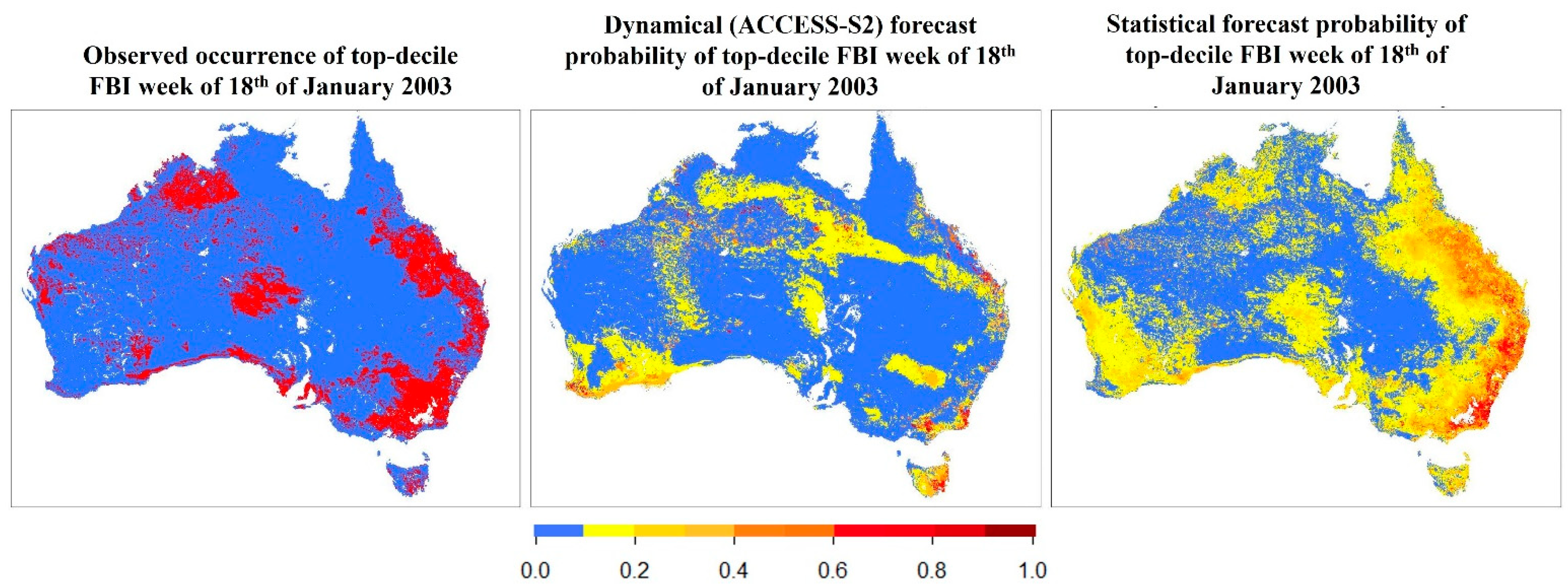
The statistical model shows a similar spatial pattern to the observed occurrence of top-decile FBI in the week of the Canberra fires (Figure 1). It clearly overpredicts the area exposed to these conditions, considering that any probability greater than 0.1 corresponds to a greater-than-climatological likelihood of extreme FBI. This overprediction is reflected in the accuracy score of 0.66. However, the areas of highest probability (~0.4 and above) closely match what was observed. The statistical model captures the high likelihood of extreme conditions along the east coast and particularly the southeast, as well as high probabilities in areas of South Australia, the Kimberly Plateau, and in a narrow strip of the Great Australian Bight. Areas where the statistical model is notably unrepresentative of the observed conditions include a large area in southwest Australia and in Tasmania, where the model shows relatively high chances of extreme FBI and these did not occur in the southwest, and occurred only in the southeast of Tasmania. The areas around Canberra, particularly at the WUI, and southeast Australia in general where the fires had the greatest impact were well highlighted by the statistical forecasting method.
The dynamical model underpredicts the chance of extreme FBI in most regions where it was observed, and predicts its occurrence in some areas where it was not. Only a small area in far southeast Victoria is predicted to experience top-decile FBI, and this does not include the Australian Capital Territory or immediate surroundings where the greatest impact of the fires was experienced. Given that the greatest impacts of fire on human-valued assets tend to occur at the WUI, the underprediction of fire danger in the region of the ACT by the dynamical model is in contrast to the performance of the statistical model in that same WUI region. This must be taken into account when considering the respective merits and drawbacks of each model, as the prediction of fire danger at the WUI may, at times, have to take precedence over prediction in other more remote areas, despite the high intrinsic value of these remote ecosystems and the services they provide. In addition to the dynamical underprediction of fire danger at the WUI, other reaches of the east coast area are also underpredicted. Similar to the statistical model, high chances of extreme FBI are predicted in the southwest by the dynamical model, where they were not observed. The dynamical model predicts a higher-than-climatological probability of extreme FBI in the northern desert regions where it was not observed nor predicted by the statistical model. The dynamical model performs notably well in Tasmania, clearly highlighting the high chances of extreme FBI that was observed in the southeast.
The dynamical model outperforms the statistical forecasting technique in terms of accuracy (Table 3—0.74 vs. 0.66). The contingency tables show that this is due to the high number of correct negatives in the dynamical model, whereas the statistical method has more hits. The statistical model performs considerably better in terms of the POD while having a similar FAR to the dynamical model, demonstrating that the statistical model is more likely to correctly issue a ‘hit’ forecast. This is consistent with the visual inspection of the dynamical and statistical forecast probabilities (Figure 1), as the statistical forecast figure shows a spatial pattern more aligned with the BARRA ground truth.
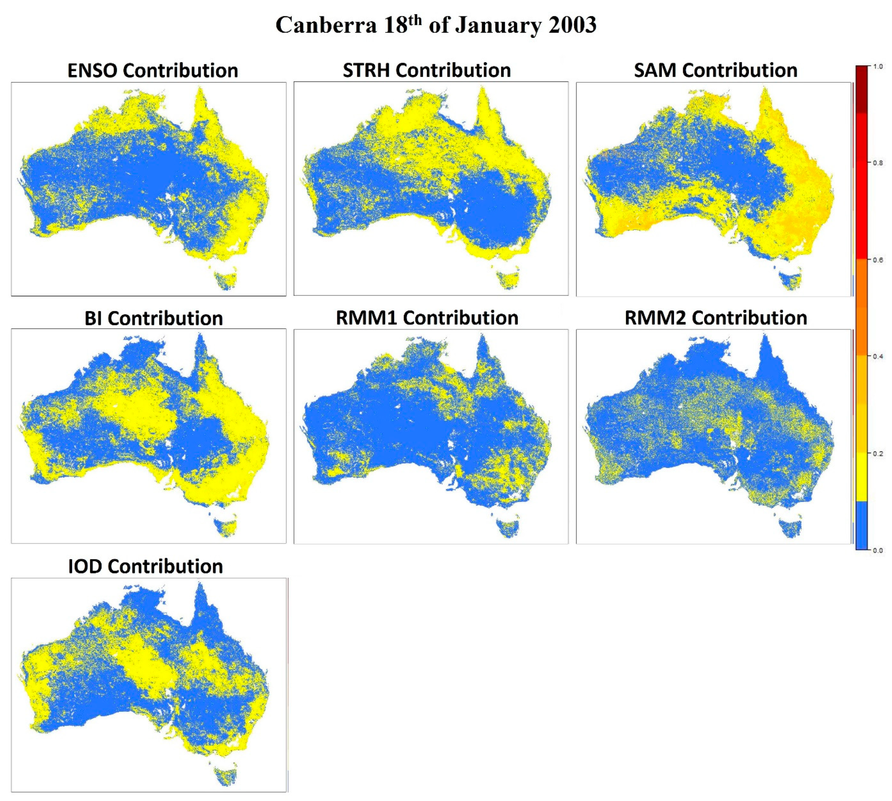
This pattern of high FBI risk reflects the compounding influences of multiple active climate drivers (Figure 2). Those likely to be most impactful in the multiple logistic regression model are the SAM, BI, and ENSO. These three climate drivers indicate a higher chance of extreme FBI on the east coast, with the SAM and BI heavily influencing the southeast. The narrow strip of high probabilities in the Great Australian Bight is evident from the contribution of STRH, and to a lesser extent, the SAM, Bi and ENSO. Finally, the increased chance of high FBI that was forecast for the southwest of the continent, but not observed, is driven most strongly by the SAM, with some contribution also from the BI and IOD. A negative SAM in DJF is associated with lower rainfall in southeast Australia [79] and higher probabilities of extreme fire conditions across the majority of the continent [20]. This is despite a lower probability of extreme heat in these regions [16]. The negative BI likewise shows an elevated chance of extreme fire danger over southern Australia in DJF [20], consistent with the reduced chances of high rainfall from cut-off low pressure systems during instances of low blocking activity [80]. This is despite its influence being lowest during the Austral summer [81]. The combination of these drivers resulting in a pattern of high risk of extreme FBI over the time of the Canberra 2003 bushfires indicates that this event was considerably influenced by the climatic conditions present at the time, which primed the landscape for a severe fire event.
Figure 1. Observed occurrence and forecasted probability of 90th percentile FBI on the week of 18 January 2003.
Atmosphere 15 00470 g001
Figure 2. Contribution of each climate driver to statistical forecast probability of 90th percentile FBI for the week of 18 January 2003 according to linear regression.
Atmosphere 15 00470 g002

3.2. Black Saturday Fires, 7 February 2009

The statistical and dynamical forecasts both show a spatial distribution of elevated chances of extreme FBI that resembles the observed distribution (Figure 3). The pattern of high probabilities in Victoria and around the margins of NSW is strongly overemphasised in the dynamical model, which contrasts with the statistical model’s failure to forecast higher probabilities of extreme FBI in northern NSW and southern QLD. Although the spatial pattern present in the southeast is well reproduced in the statistical model, the magnitude of the signal is much less than what is forecast by the dynamical model. On the other hand, the distribution of high chances of extreme FBI in central Australia is notably more accurate in the statistical than the dynamical model. Both modelling methods additionally forecast high chances of extreme FBI on parts of the west coast, which is not consistent with the observed results. In this case, although a total of over 400 fires were recorded, many of these occurred elsewhere, away from the WUI. A total of 73 fires impacted communities by burning at or through the WUI, and it is at the locations of such impacts that accurate model prediction would have been most valuable. Most notably, the Kilmore East and Kinglake fire complexes were those which resulted in the greatest damages to communities. That being said, these case studies do represent only a window in time, and where extreme fire danger is present, many other factors, such as ignition and short-term atmospheric and fuel attributes, have a major influence on potential fire damage. In this case, it is evident that although the dynamical model predicts a very high likelihood of extreme fire danger in Victoria and southeast Australia, the exact spatial distribution and pattern of extreme fire weather is more closely replicated by the statistical model, despite its lower probability magnitude. This suggests that the statistical model’s spatial accuracy in this region may have been of considerable benefit to fire management, given the amount of WUI land that was affected here.
The statistical model displays higher performance scores than the dynamical model in terms of accuracy, with an identical POD (Table 4). Both have similar forecast hits, but the statistical model results include more correct negatives and fewer false alarms. However, the statistical model also has a lower false alarm ratio, which may indicate a more accurate forecast overall.
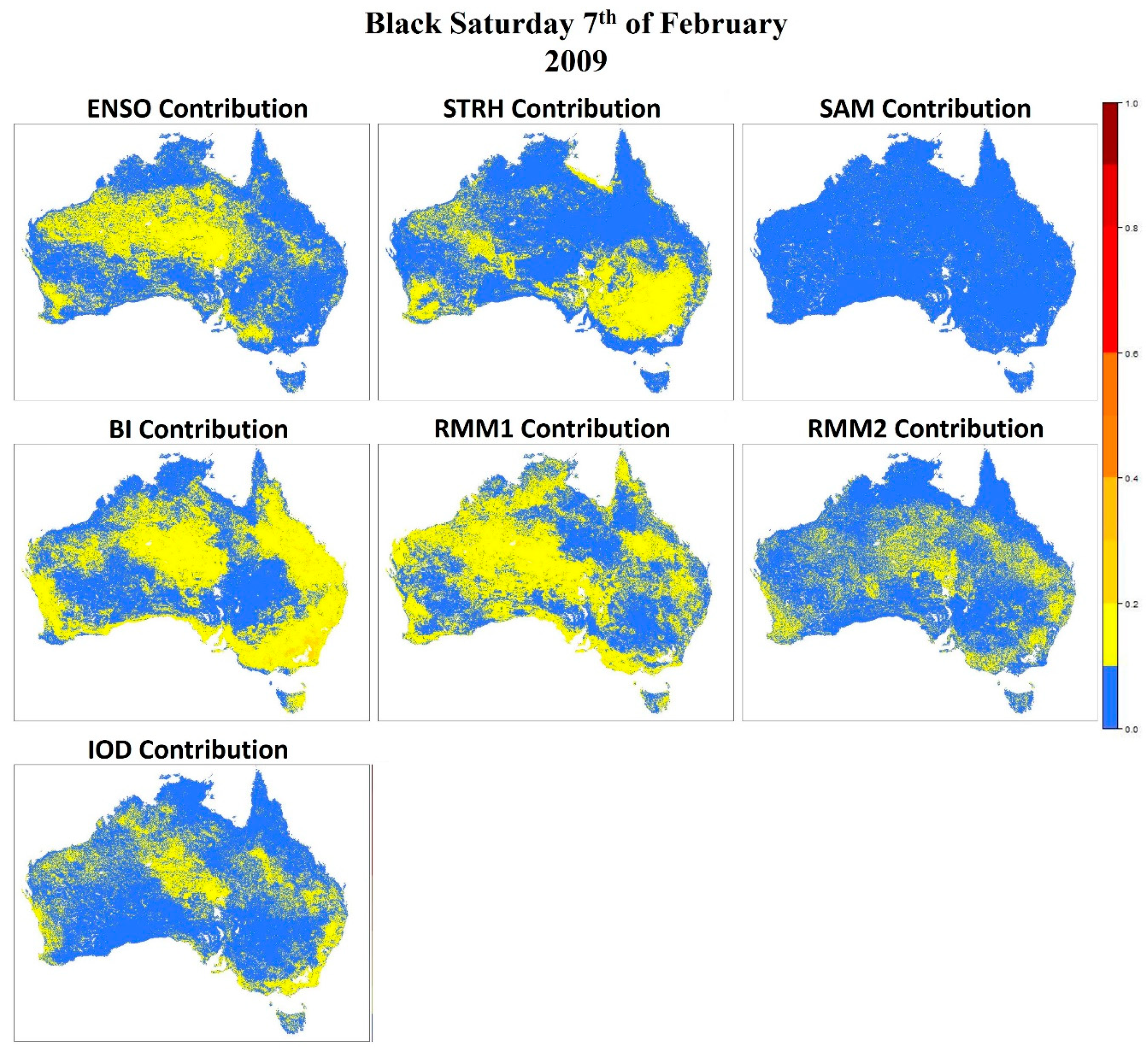
The climate drivers contributing to the pattern shown by the statistical forecast model are predominantly the ENSO, BI, and RMM1 (Figure 4). A strong negative BI was present in this case and, hence, the influence of the BI is similar to that in the Canberra 2003 case study. A strong RMM1 was also present, corresponding to MJO phases 4 and 5. The pattern displayed for the influence of RMM1 reflects the observed impacts of MJO phase 4 on FFDI in the southern reaches of Australia, and to some extent, the impacts of phase 5 that are simulated by the ACCESS-S1 model in parts of central and western Australia [19]. The ENSO was in a negative (La Niña) phase in February 2009, which is significant because extreme fire events are usually associated with an El Niño event in Australia [82,83,84,85]. Hence, the influence of the ENSO in this case is consistent with that of a La Niña phase, when fire risk is increased in the central desert areas of Australia due to increased biomass growth [86,87,88]. The region of the strongest BI and RMM1 interaction correlates well with the region of increased probability of extreme FBI that is observed in central Australia. During this event, the STRH was in a strongly positive phase. Its lack of evidence in the statistical logistic regression forecast is unexpected, and is thought to be due to its influence being negated by the influence of the other drivers assessed, which generally act to reduce the chance of extreme FBI in central southeast Australia. Overall, although the accuracy metrics for the statistical model are high, the strong ability of ACCESS-S2 to highlight the increased chance of severe FBI, particularly in the affected region of Victoria, indicates that the FBI was considerably influenced by shorter-term meteorological factors that are less represented by large-scale climate drivers [68,71].

3.3. Pinery Fire, 25 November 2015

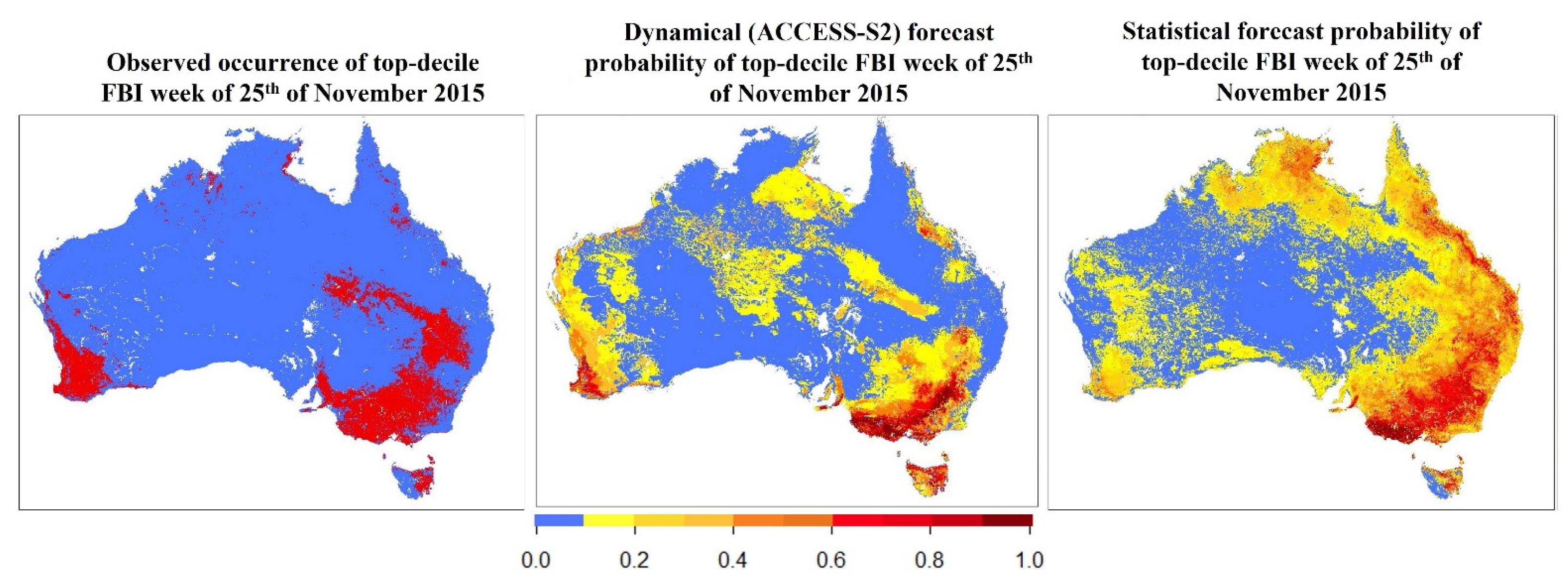
There is a discrepancy between the dynamical and statistical forecasts of the extreme FBI probability in the week of the Pinery fire case study (Figure 5). The statistical forecast model indicates a very high likelihood of extreme FBI in the southeast of Australia and up the east coast. In some locations, this likelihood is greater than 0.9. Increased chances of extreme FBI are also forecast in northern Australia and the southwest. In contrast, the dynamical model indicates higher chances of extreme FBI being most likely in southeast Australia, southwest western Australia and Tasmania, with limited probability of extreme fire danger elsewhere. Both models capture the increase in the probability of extreme FBI in the regions north of Adelaide, which were impacted at the WUI by the fire event, and in southwest Australia, which was impacted by fires in the preceding week [89]. The statistical model clearly highlights the risk of high FBI in southeast Australia in the region of the fires, as well as the observed signal through eastern Tasmania, eastern NSW and southern QLD. However, it substantially overpredicts the chance of severe FBI, particularly in QLD and northern Australia, where it was not observed. In this case, both models capture different elements of the observed spatial distribution of extreme FBI, highlighting the value of having more than one forecasting method for such events.
The differences described above are represented in the contingency tables for the statistical and dynamical models (Table 5). The accuracy of the dynamical model is higher than that of the statistical model. This can be partially attributed to the higher proportion of correct negatives, while it can be seen that the statistical model displays more hits and fewer misses. The false alarm ratio is once again higher in the statistical model, but not by a large margin, while the probability of detection is far higher in the statistical model as opposed to the dynamical forecast. As we discuss in Section 4, this discrepancy can highlight the importance of assessing more than one model’s output for a fire danger forecast, particularly when operational agencies are aware in advance that extreme conditions are likely [90].
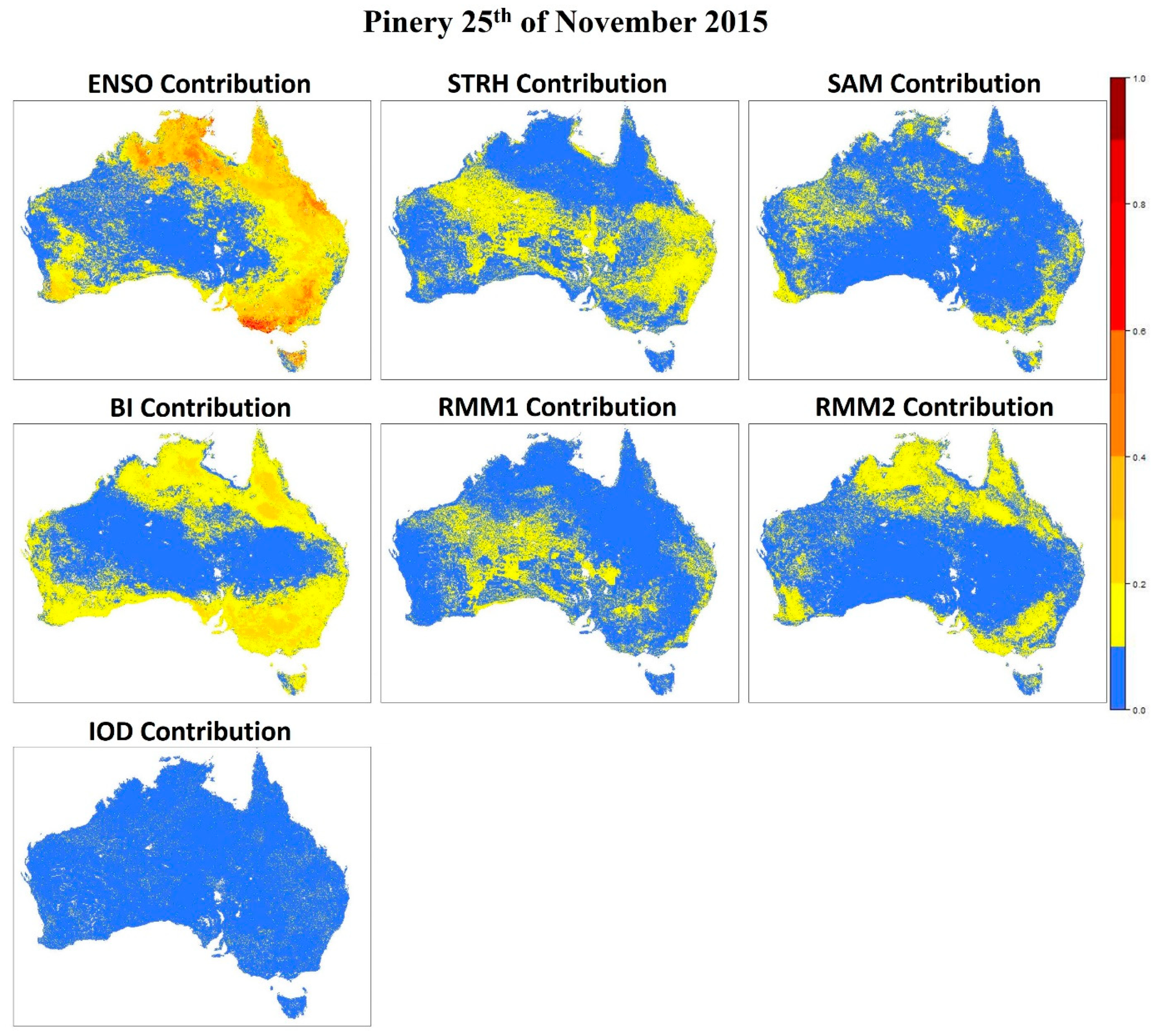
In this case, the primary influence on the chance of extreme FBI is the ENSO (Figure 6), which was in a strong El Niño phase, with an ENSO3.4 index more than two standard deviations above the 2003–2017 mean. This results in a strong signal of increased chances of extreme FBI, which closely resembles the distribution in the full logistic regression forecast (Figure 5). This is consistent with the expected influence of El Niño on heat and rainfall [15,91] and, hence, fire danger in Australia [20]. The BI also adds to the magnitude of the signal in southern and northern Australia. Further amplification of the signal in southeast, southwest, and northern Australia is due to the positive RMM2, indicating MJO phases 6 and 7. In SON, MJO phase 6 is strongly associated with increased chances of severe fire weather, particularly in southwest Australia, whereas phase 7 is more influential in inland Australia [19]. However, rainfall is more significantly decreased in southwest Australia during phase 7 of the MJO in SON [92], so both of these phases may contribute to the statistically modelled signal. the Climate outlooks for the period leading up to spring in 2015 also suggested below-average rainfall and above-average temperatures in northern Australia [93], so the fact that this was not observed may be an anomaly compared to the usual influences of the climate drivers active at the time.

4. Discussion

Our case studies and investigations demonstrate that neither ACCESS-S2 nor a logistical regression approach is capable of accurately forecasting the occurrence of top-decile fire danger at two- to three-week lead times. However, the current FBI outlooks are driven solely by ACCESS-S2 and fuel information, and ACCESS-S2 outlooks have historically produced underestimates of cases of extreme FBI, as also demonstrated in the case studies above. Conversely, using a statistical approach solely based on climate driver activity results in overprediction of the area affected by extreme FBI. The inclusion of fuel information in official outlooks is one way in which the ACCESS-S2 forecasts are considerably more advantageous; however, these extreme tails of the distribution are often not well represented by climate models [94].
A model which uses climate driver information as its inputs may also have value for the advanced forecasting of extreme fire danger conditions at longer time scales than what may be practical with dynamical models. Climate driver states are often accurately predicted by ACCESS-S2 up to six months in advance, with understandably shorter lead times for drivers with a shorter overall period [21]. The extent to which an outlook can be extended may depend on the strength of the relationships between a climate driver and extreme fire danger in the region of interest. For example, in an area where the effect of ENSO is highly significant, but the influence of RMM indices are insignificant, it may be possible to achieve longer lead times of 1–6 months, depending on the season [21]. In contrast, where the MJO or the SAM is found to be a dominant driver, or in cases of very high amplitudes of these events, the achievable lead time may be shorter, in the order of approximately 15 days. This has potential to add value for fire practitioners and diverse stakeholders.
Extended lead times can be used beneficially through a hybrid forecasting approach whereby dynamically driven climate driver data can be entered into the statistical model [95]. Hybrid forecasting usually takes the form of combining time-series forecasting with a machine learning model [96]. However, the use of dynamically derived predictions as the input to a statistical model is a commonly used approach at a subseasonal to seasonal timescale [97]. Analysing the output from such a hybrid forecast, a climate-state-driven statistical model of the probability of extreme FBI for a period several weeks to months ahead may prove valuable for giving an additional or earlier indication of the expected severity of an upcoming fire season, or, for example, planning suitable windows for preparatory activities such as planned burns, which must be scheduled far in advance. There are also other methods of constructing hybrid, merged, or paired predictive models which may prove highly valuable for this case. Most notably, the approach taken by Schepen and Wang [98] presents a solution for analyses quite similar to those presented here. Schepen and Wang utilised Bayesian Model Averaging to combine a climate-driver-driven statistical rainfall forecast with a GCM rainfall forecast, showing that the combined model considerably outperforms both the dynamical and the statistical model. This method for combining the strengths of both models is likely to be a fruitful pathway for further investigation in this field of fire danger forecasting. Future research could investigate the potential for Artificial Intelligence (AI) in developing or combining the models’ strengths; however, the rapid evolution of AI as a field puts a complete review of this possibility beyond the scope of our study. One further avenue to consider is the possibility of explicitly accounting for climate drivers in the AFDRS as a whole. Fire management practitioners confirm that there is “room left” in the system for the inclusion of climate states, but that these have not yet been incorporated [99]. This study offers a potential model through which to incorporate climate driver relationships into AFDRS models.
The use of the BARRA climatology as an ‘observed’ reference point introduces an added limitation to our analysis. This is because there are notable uncertainties embedded in the climatology, which cannot be quantified. These uncertainties include the following:
  • The finalisation of the climatology in March 2023. The AFDRS is a modular system, designed to be updated and improved upon over time. As weaknesses and limitations are identified in the operation of the system, changes are likely to be made to the fuel models which will not be reflected in the climatology and hindcasts used in our study.
  • In some fuel types, adaptions were made to existing fuel state models to attempt to account for the unavailability of an accurate fuel state history. These adaptations did not always have a strong scientific basis and may therefore introduce an element of error into the observed values [55].
  • The limited climatology of 2003–2017 confines the analysis to a warmer and wetter period than the average climate state [100,101], in addition to introducing weaknesses due to it being shorter than an official climatology definition of 30 years.
Uncertainties implicit in the BARRA reanalysis model are accounted for as discussed by Su and Eizenberg [102].
In cases such as extreme fire danger conditions, where impacts can be significant, there may be value in considering the ‘worst case’ scenario suggested in the statistical model, in conjunction with what was shown by the official FBI outlook. The McLeod Inquiry which followed the 2003 bushfires criticised authorities for ‘reassuring’ the public, rather than presenting ‘a more sober and realistic estimation of the dangers that might lie ahead’ [103]. Inquiries following this and more recent events also recommended more preparation for extreme fire seasons, despite acknowledging some improvements over time [103,104,105,106,107]. These criticisms may be mitigated in future, and communities can be more aware of and prepared for severe fire events, if additional prediction methods are considered in conjunction with the official forecasts. However, it is important to balance this with the costs, both financial and social, of overpreparing for extreme fire seasons. Clearly, the presence of a high FBI does not guarantee the ignition of a fire or development of the fire into a threat to life and property, and preparation and the associated costs may be seen as unnecessary in response to high fire danger if ignitions do not occur. For example, the recruitment of aerial resources, other firefighting equipment, and human resources is costly. Over the 2018–2019 financial year, the New South Wales Rural Fire Service spent AUD 11 million on mitigation and resilience, most of which was allocated to the maintenance of fire trails and planned burning [108]. The cost of aerial suppression equipment is cited at approximately 1800 AUD/hour for a small helicopter and approximately 35,000 AUD/hour for larger air tankers, without accounting for the costs of crew, fuel, and retardant (ibid). These resources are also costly to keep on standby, with fleet standby costs of AUD 18 million (2008–2009 value) in Victoria over the 2008–2009 financial year [109]. Such expenses associated with the recruitment and readiness of these resources may be unacceptable to the public and to governments when routinely carried out in response to a false alarm. Hazard-reduction burning also has a large financial and labour cost, and also produces a smoke burden which impacts public health and other industries. All these considerations must be balanced with the awareness of the costs of fighting and recovering from severe fire seasons, including not only the direct financial costs, but also the environmental, social, health, heritage, psychological, and intangible costs.
Socially, the continued issuing of warnings related to high fire danger and warnings to the community can result in warning fatigue when extreme fire events do not arise. This can result in not only community discontent but also ‘cynicism and apathy’ [110]. For this reason, it is important to remain aware of the high false alarm ratio which regularly accompanies statistical model forecasts. However, underexpressing the risk to the community is also socially unacceptable, and an appropriate balance between warning fatigue and underwarning should be the aim. Thus, it is of critical importance to consider methods for combining the two forecasts, such as the Bayesian Model Averaging approach used by Schepen and Wang [98]. Meanwhile, given the discrepancy often present between the statistical and dynamical model outlooks, carefully analysing both, with input from on-the-ground operational agencies, may aid in reaching an appropriate balance more often.
These case studies offer limited examples of the model’s performance. They serve to showcase three impactful events in South Australia in this region’s active fire season of spring and summer [111]. The statistical model may produce varying results in other areas of Australia, depending on the ability of a linear method to capture relationships between fire danger and climate influences. For instance, where climate drivers may have a less pronounced or less clear influence on fire danger [20], a linear model may prove less effective. This also holds for regions and fire seasons where multicollinearity and teleconnections between drivers are different or have different strengths [83,112,113]. In these cases, there may be benefits in considering other non-linear forms of forecasting, such as more developed machine-learning models, or the AI-based methods alluded to above. Further, in certain seasons, the occurrence or impact of some climate drivers is different to what it is in the Austral spring and summer, e.g., [15,19,20]. For regions such as northern and central Australia, where fires are most active or destructive during other months of the year [111], the model structure could be compromised. However, as the probability of extreme fire danger in northern regions of Australia is generally highly predictable from climate activity [43], this is unlikely to introduce significant errors or weaknesses.

5. Conclusions

This study investigates the capabilities of two distinct approaches for forecasting extreme danger (represented by the top-decile Fire Behaviour Index): the Australian Community Climate and Earth-System Simulator (ACCESS-S2) and a newly developed statistical model driven by climate drivers. Both models demonstrated both strengths and limitations in accurately predicting these rare events at two- to three-week lead times.
ACCESS-S2, while reliable for general fire danger trends, underestimated extreme FBI events in the case studies, potentially impacting community preparedness during high-risk periods. Conversely, the statistical model exhibited sensitivity to climate driver activity, but overpredicted of the area affected by extreme FBI, as demonstrated by the generally high probability of detection and false alarm ratio scores. If such a model were relied upon for estimating the probability of extreme fire danger, it would potentially raise concerns about false alarms and resource mismanagement.
These findings highlight the challenge of balancing accuracy and overwarning in fire danger forecasting. Underestimating risk leaves communities vulnerable, while overestimating it can trigger unnecessary resource allocation and disrupt daily life. Therefore, we propose the following strategies to improve forecasting and communication:
  • Combined analysis involving Integrating ACCESS-S2 and statistical model forecasts with on-the-ground expertise can provide a more comprehensive picture of potential fire danger, enabling nuanced risk assessments;
  • Further research into avenues for combining dynamical and statistical forecast strengths, such as Bayesian Model Averaging or potential AI-based approaches, presents the opportunity to develop a single prediction system which explicitly accounts for the statistical relationships between fire danger and climate drivers, while additionally considering the factors captured by the dynamical model;
  • Operational integration involving investigating strategies to incorporate the statistical model’s “worst case” scenarios into official outlooks, such as probabilistic forecasts or scenario planning, can help better prepare for extreme events without triggering widespread false alarms;
  • Transparent communication involving clearly communicating the limitations and uncertainties of each forecast, the potential consequences of overwarning and underwarning, and the rationale behind risk assessments can maintain public trust and understanding.
Mitigating the impacts of extreme fire events requires a multifaceted approach that acknowledges the limitations of current forecasting models while leveraging their strengths. By integrating climate knowledge, dynamical models, statistical forecasts, and on-the-ground expertise, we can improve the accuracy of fire danger warnings, optimise resource allocation, and build resilience in fire-prone communities.

Author Contributions

Conceptualisation, R.T., A.G.M., and S.C.; methodology, R.T.; validation, R.T.; formal analysis, R.T.; investigation, R.T.; data curation, R.T.; writing—original draft preparation, R.T.; writing—review and editing, R.T., A.G.M., S.C., G.J.C., and S.H.; visualisation, R.T.; supervision, A.G.M., S.C., G.J.C., and S.H. All authors have read and agreed to the published version of the manuscript.

Funding

This research received no external funding.

Institutional Review Board Statement

Not applicable.

Informed Consent Statement

Not applicable.

Data Availability Statement

Due to its proprietary nature, the supporting AFDRS data are available solely for research and teaching purposes and to government agencies upon request to AFAC at [email protected]. Further information about the data and conditions for access are available in the National Computational Infrastructure Data Catalogue at https://geonetwork.nci.org.au/geonetwork/srv/eng/catalog.search#/metadata/f3311_4920_0252_8073 (accessed on: 26 March 2024).

Acknowledgments

This work was undertaken with the assistance of resources from the National Computational Infrastructure (NCI), which is supported by the Australian Government. We extend our thanks to the Bureau of Meteorology ACCESS-S team [21] for their work on the production and management of the ACCESS-S2 hindcasts, to Samuel Sauvage for his work on the BARRA AFDRS Climatology, and to Paul Gregory for his work on the AFDRS hindcasts at the Bureau of Meteorology.

Conflicts of Interest

The authors declare no conflicts of interest.

References

  1. Kanowski, P.J.; Whelan, R.J.; Ellis, S. Inquiries following the 2002–2003 Australian bushfires: Common themes and future directions for Australian bushfire mitigation and management. Aust. For. 2005, 68, 76–86. [Google Scholar] [CrossRef]
  2. Teague, B.; Pascoe, S.; McLeod, R. The 2009 Victorian Bushfires Royal Commission Final Report: Summary; Government Printer for the State of Victoria: Melbourne, Australia, 2010.
  3. Zimmermann, A.; Pinery Fire Recovery Final Report. South Australia. 2017. Available online: https://dhs.sa.gov.au/__data/assets/pdf_file/0007/57418/2015-Pinery-Fire-Recovery-Report.pdf (accessed on 17 February 2024).
  4. Hefferman, B.; O’Brien, K.; Fisher, M.J.; Milne, C.; Nash, F.; Sterle, G.; Back, C.; Colbeck, R. The Incidence and Severity of Bushfires across Australia—Chapter 2: Previous Bushfire Inquiries; Senate Printing Unit: Canberra, Australia, 2009. Available online: https://www.aph.gov.au/Parliamentary_Business/Committees/Senate/Former_Committees/agric/completed_inquiries/2008-10/bushfires/report/c02 (accessed on 24 February 2024).
  5. Canadell, J.G.; Meyer, C.P.; Cook, G.D.; Dowdy, A.; Briggs, P.R.; Knauer, J.; Pepler, A.; Haverd, V. Multi-decadal increase of forest burned area in Australia is linked to climate change. Nat. Commun. 2021, 12, 6921. [Google Scholar] [CrossRef]
  6. Moreira, F.; Ascoli, D.; Safford, H.; Adams, M.A.; Moreno, J.M.; Pereira, J.M.; Catry, F.X.; Armesto, J.; Bond, W.; González, M.E. Wildfire management in Mediterranean-type regions: Paradigm change needed. Environ. Res. Lett. 2020, 15, 011001. [Google Scholar] [CrossRef]
  7. Harris, S.; Mills, G.; Brown, T. Variability and drivers of extreme fire weather in fire-prone areas of south-eastern Australia. Int. J. Wildland Fire 2017, 26, 177–190. [Google Scholar] [CrossRef]
  8. Storey, M.; Price, O.; Tasker, E. The role of weather, past fire and topography in crown fire occurrence in eastern Australia. Int. J. Wildland Fire 2016, 25, 1048–1060. [Google Scholar] [CrossRef]
  9. Bradstock, R.A.; Cohn, J.; Gill, A.M.; Bedward, M.; Lucas, C. Prediction of the probability of large fires in the Sydney region of south-eastern Australia using fire weather. Int. J. Wildland Fire 2010, 18, 932–943. [Google Scholar] [CrossRef]
  10. Bradstock, R.A. A biogeographic model of fire regimes in Australia: Current and future implications. Glob. Ecol. Biogeogr. 2010, 19, 145–158. [Google Scholar] [CrossRef]
  11. Gill, A.M.; Stephens, S.L.; Cary, G.J. The worldwide “wildfire” problem. Ecol. Appl. 2013, 23, 438–454. [Google Scholar] [CrossRef]
  12. O’Connor, C.D.; Calkin, D.E.; Thompson, M.P. An empirical machine learning method for predicting potential fire control locations for pre-fire planning and operational fire management. Int. J. Wildland Fire 2017, 26, 587–597. [Google Scholar] [CrossRef]
  13. Penman, T.D.; Cirulis, B.A. Cost effectiveness of fire management strategies in southern Australia. Int. J. Wildland Fire 2020, 29, 427–439. [Google Scholar] [CrossRef]
  14. Blanchi, R.; Lucas, C.; Leonard, J.; Finkele, K. Meteorological conditions and wildfire-related houseloss in Australia. Int. J. Wildland Fire 2010, 19, 914–926. [Google Scholar] [CrossRef]
  15. Risbey, J.S.; Pook, M.J.; McIntosh, P.C.; Wheeler, M.C.; Hendon, H.H. On the Remote Drivers of Rainfall Variability in Australia. Mon. Weather Rev. 2009, 137, 3233–3253. [Google Scholar] [CrossRef]
  16. Marshall, A.G.; Hudson, D.; Wheeler, M.C.; Alves, O.; Hendon, H.H.; Pook, M.J.; Risbey, J.S. Intra-seasonal drivers of extreme heat over Australia in observations and POAMA-2. Clim. Dyn. 2014, 43, 1915–1937. [Google Scholar] [CrossRef]
  17. Marshall, A.G.; Wang, G.M.; Hendon, H.H.; Lin, H. Madden-Julian Oscillation teleconnections to Australian springtime temperature extremes and their prediction in ACCESS-S1. Clim. Dyn. 2023, 61, 431–447. [Google Scholar] [CrossRef]
  18. Marshall, A.G.; Wheeler, M.C.; Cowan, T. Madden-Julian Oscillation Impacts on Australian Temperatures and Extremes. J. Clim. 2023, 36, 335–357. [Google Scholar] [CrossRef]
  19. Marshall, A.G.; Gregory, P.A.; de Burgh-Day, C.O.; Griffiths, M. Subseasonal drivers of extreme fire weather in Australia and its prediction in ACCESS-S1 during spring and summer. Clim. Dyn. 2021, 58, 523–533. [Google Scholar] [CrossRef]
  20. Taylor, R.; Marshall, A.G.; Crimp, S.; Cary, G.J.; Harris, S.; Sauvage, S. Associations between Australian climate drivers and extreme weekly fire danger. Int. J. Wildland Fire 2023, 33, WF23060. [Google Scholar] [CrossRef]
  21. Wedd, R.; Alves, O.; de Burgh-Day, C.; Down, C.; Griffiths, M.; Hendon, H.H.; Hudson, D.; Li, S.; Lim, E.-P.; Marshall, A.G.; et al. ACCESS-S2: The upgraded Bureau of Meteorology multi-week to seasonal prediction system. J. South. Hemisph. Earth Syst. Sci. 2022, 72, 218–242. [Google Scholar] [CrossRef]
  22. Moritz, M.A.; Batllori, E.; Bradstock, R.A.; Gill, A.M.; Handmer, J.; Hessburg, P.F.; Leonard, J.; McCaffrey, S.; Odion, D.C.; Schoennagel, T.; et al. Learning to coexist with wildfire. Nature 2014, 515, 58–66. [Google Scholar] [CrossRef]
  23. Hagmann, R.K.; Hessburg, P.F.; Salter, R.B.; Merschel, A.G.; Reilly, M.J. Contemporary wildfires further degrade resistance and resilience of fire-excluded forests. For. Ecol. Manag. 2022, 506, 119975. [Google Scholar] [CrossRef]
  24. Feng, P.; Wang, B.; Li Liu, D.; Ji, F.; Niu, X.; Ruan, H.; Shi, L.; Yu, Q. Machine learning-based integration of large-scale climate drivers can improve the forecast of seasonal rainfall probability in Australia. Environ. Res. Lett. 2020, 15, 084051. [Google Scholar] [CrossRef]
  25. Rasel, H.; Imteaz, M.; Mekanik, F. Investigating the influence of Remote Climate Drivers as the Predictors in Forecasting South Australian spring rainfall. Int. J. Environ. Res. 2016, 10, 1–12. [Google Scholar]
  26. Furman, J.H.; Linn, R.R. What is FIRETEC (and why should I care)? Fire Manag. Today 2018, 76, 33–36. [Google Scholar]
  27. Walker, J. PHOENIX Rapidfire Knowledge Base. 2018. Available online: https://firepredictions.atlassian.net/wiki/spaces/viewspacesummary.action?key=PH (accessed on 22 March 2024).
  28. Spark Operational Features. 2023. Available online: https://www.afac.com.au/docs/default-source/fire-predictions/spark-operational-_-features.pdf?sfvrsn=2 (accessed on 22 March 2024).
  29. Juliano, T.W.; Lareau, N.; Frediani, M.E.; Shamsaei, K.; Eghdami, M.; Kosiba, K.; Wurman, J.; DeCastro, A.; Kosović, B.; Ebrahimian, H. Toward a Better Understanding of Wildfire Behavior in the Wildland-Urban Interface: A Case Study of the 2021 Marshall Fire. Geophys. Res. Lett. 2023, 50, e2022GL101557. [Google Scholar] [CrossRef]
  30. Hossain, I.; Rasel, H.M.; Imteaz, M.A.; Mekanik, F. Long-term seasonal rainfall forecasting using linear and non-linear modelling approaches: A case study for Western Australia. Meteorol. Atmos. Phys. 2020, 132, 131–141. [Google Scholar] [CrossRef]
  31. Hossain, I.; Esha, R.; Alam Imteaz, M. An Attempt to Use Non-Linear Regression Modelling Technique in Long-Term Seasonal Rainfall Forecasting for Australian Capital Territory. Geosciences 2018, 8, 282. [Google Scholar] [CrossRef]
  32. Mekanik, F.; Imteaz, M.A. Forecasting Victorian spring rainfall using ENSO and IOD: A comparison of linear multiple regression and nonlinear ANN. In Proceedings of the 2012 2nd International Conference on Uncertainty Reasoning and Knowledge Engineering, Jalarta, Indonesia, 14–15 August 2012; pp. 86–89. [Google Scholar] [CrossRef]
  33. Rasel, H.; Imteaz, M. Application of Artificial Neural Network for seasonal rainfall forecasting: A case study for South Australia. In Proceedings of the World Congress on Engineering, London, UK, 29 June–1 July 2016; Available online: https://www.iaeng.org/publication/WCE2016/WCE2016_pp130-134.pdf (accessed on 18 January 2024).
  34. Bagirov, A.M.; Mahmood, A.; Barton, A. Prediction of monthly rainfall in Victoria, Australia: Clusterwise linear regression approach. Atmos. Res. 2017, 188, 20–29. [Google Scholar] [CrossRef]
  35. Khastagir, A.; Hossain, I.; Anwar, A.H.M.F. Efficacy of linear multiple regression and artificial neural network for long-term rainfall forecasting in Western Australia. Meteorol. Atmos. Phys. 2022, 134, 69. [Google Scholar] [CrossRef]
  36. Richman, M.B.; Leslie, L.M. Attribution and Prediction of Maximum Temperature Extremes in SE Australia. Procedia Comput. Sci. 2014, 36, 612–617. [Google Scholar] [CrossRef]
  37. McKay, R.; Bettio, L.; Wang, W.; Ramchurn, A.; Hope, P. Multi-Linear Regression to Explain Australian Climate Events. In Proceedings of the Bureau of Meteorology Annual R&D Workshop: Towards Seasmless Science and Services, Melbourne, Australia, 7–10 August 2023; Available online: http://www.bom.gov.au/research/workshop/2023/posters/RoseannaMcKay_poster.pdf (accessed on 30 January 2024).
  38. Tozer, C.R.; Kiem, A.S.; Verdon-Kidd, D.C. Large-scale ocean-atmospheric processes and seasonal rainfall variability in South Australia: Potential for improving seasonal hydroclimatic forecasts. Int. J. Climatol. 2017, 37, 861–877. [Google Scholar] [CrossRef]
  39. Palmer, T.N. A nonlinear dynamical perspective on climate prediction. J. Clim. 1999, 12, 575–591. [Google Scholar] [CrossRef]
  40. Rial, J.A.; Pielke, R.A.; Beniston, M.; Claussen, M.; Canadell, J.; Cox, P.; Held, H.; de Noblet-Ducoudré, N.; Prinn, R.; Reynolds, J.F. Nonlinearities, feedbacks and critical thresholds within the Earth’s climate system. Clim. Chang. 2004, 65, 11–38. [Google Scholar] [CrossRef]
  41. Westra, S.; Sharma, A. An upper limit to seasonal rainfall predictability? J. Clim. 2010, 23, 3332–3351. [Google Scholar] [CrossRef]
  42. Power, S.; Haylock, M.; Colman, R.; Wang, X. The predictability of interdecadal changes in ENSO activity and ENSO teleconnections. J. Clim. 2006, 19, 4755–4771. [Google Scholar] [CrossRef]
  43. Taylor, R.; Marshall, A.G.; Crimp, S.; Cary, G.J.; Harris, S. Climate Driver Influences on Prediction of the Australian Fire Behaviour Index. Atmosphere 2024, 15, 203. [Google Scholar] [CrossRef]
  44. Schug, F.; Bar-Massada, A.; Carlson, A.R.; Cox, H.; Hawbaker, T.J.; Helmers, D.; Hostert, P.; Kaim, D.; Kasraee, N.K.; Martinuzzi, S.; et al. The global wildland–urban interface. Nature 2023, 621, 94–99. [Google Scholar] [CrossRef] [PubMed]
  45. Bento-Gonçalves, A.; Vieira, A. Wildfires in the wildland-urban interface: Key concepts and evaluation methodologies. Sci. Total Environ. 2020, 707, 135592. [Google Scholar] [CrossRef] [PubMed]
  46. Price, O.; Bradstock, R. The spatial domain of wildfire risk and response in the Wildland Urban Interface in Sydney, Australia. Nat. Hazards Earth Syst. Sci. 2013, 13, 3385–3393. [Google Scholar] [CrossRef]
  47. Kalnay, E.; Kanamitsu, M.; Kistler, R.; Collins, W.; Deaven, D.; Gandin, L.; Iredell, M.; Saha, S.; White, G.; Woollen, J. The NCEP/NCAR 40-year reanalysis project. Bull. Am. Meteorol. Soc. 1996, 77, 437–471. [Google Scholar] [CrossRef]
  48. Wheeler, M.C.; Hendon, H.H. An All-Season Real-Time Multivariate MJO Index: Development of an Index for Monitoring and Prediction. Mon. Weather Rev. 2004, 132, 1917–1932. [Google Scholar] [CrossRef]
  49. Trenberth, K.E. The Definition of El Niño. Bull. Am. Meteorol. Soc. 1997, 78, 2771–2778. [Google Scholar] [CrossRef]
  50. Saji, N.H.; Yamagata, T. Possible impacts of Indian Ocean Dipole mode events on global climate. Clim. Res. 2003, 25, 151–169. [Google Scholar] [CrossRef]
  51. Gong, D.; Wang, S. Definition of Antarctic oscillation index. Geophys. Res. Lett. 1999, 26, 459–462. [Google Scholar] [CrossRef]
  52. Pook, M.; Gibson, T. Atmospheric blocking and storm tracks during SOP-1 of the FROST Project. Aust. Meteorol. Mag. 1999, 48, 51–60. [Google Scholar]
  53. AFAC. Australian Fire Danger Rating System Frequently Asked Questions (FAQs). Available online: https://www.afac.com.au/initiative/afdrs/afdrs-faqs (accessed on 30 January 2024).
  54. Cube Management Solutions. Improving Our National Fire Danger Rating System. 2014. Available online: https://www.afac.com.au/docs/default-source/afdrs/nfdrs---concept-document-v1-0-final.pdf?sfvrsn=2 (accessed on 24 November 2023).
  55. Matthews, S. Fire Behaviour Index Technical Guide. 2022. Available online: https://www.afac.com.au/docs/default-source/afdrs/fire-behaviour-index-technical-guide.pdf?sfvrsn=4&download=true (accessed on 29 February 2024).
  56. Gregory, P.; Bureau of Meteorology, Docklands, Australia. Your AFDRS hindcast query. Personal communication, 12 December 2023.
  57. Matthews, S.; NSW Rural Fire Service, Sydney Olympic Park & Nova Systems, 100 William Street, Woolloomooloo 2011, Australia. RE: Enquiries regarding fuel loads in the AFDRS. Personal communication, 7 October 2023.
  58. Australian Bureau of Meteorology. Bureau of Meteorology Fire Behaviour Model Guides. Available online: https://www.afac.com.au/initiative/afdrs/article/bom-fire-behaviour-model-guides (accessed on 24 November 2023).
  59. Matthews, S.; Fox-Hughes, P.; Grootemaat, S.; Hollis, J.J.; Kenny, B.J.; Sauvage, S. Australian Fire Danger Rating System: Research Prototype; NSW Rural Fire Service: Lidcombe, Australia, 2019. Available online: https://www.afac.com.au/docs/default-source/afdrs/afdrs_research_prototype_report_2019.pdf?sfvrsn=6 (accessed on 29 February 2024).
  60. Hudson, D.; Alves, O.; Hendon, H.H.; Lim, E.-P.; Liu, G.; Luo, J.-J.; MacLachlan, C.; Marshall, A.G.; Shi, L.; Wang, G. ACCESS-S1 the new Bureau of Meteorology multi-week to seasonal prediction system. J. South. Hemisph. Earth Syst. Sci. 2017, 67, 132–159. [Google Scholar] [CrossRef]
  61. Collaboration for Australian Weather and Climate Research. Forecast Verification Issues, Methods and FAQ. In Proceedings of the 7th International Verification Methods Workshop, Berlin, Germany, 3–10 May 2015; Available online: https://www.cawcr.gov.au/projects/verification/ (accessed on 10 January 2024).
  62. Bureau of Meteorology. About the Long Range Forecasts: Accuracy. Available online: http://www.bom.gov.au/climate/ahead/about/index.shtml#tabs=Accuracy (accessed on 8 January 2024).
  63. Camilleri, P.; Healy, C.; Macdonald, E.; Nicholls, S.; Sykes, J.; Winkworth, G.; Woodward, M. Recovery from bushfires: The experience of the 2003 Canberra bushfires three years after. Australas. J. Paramed. 2010, 8, 1–15. [Google Scholar] [CrossRef]
  64. McRae, R.H.; Sharples, J.J.; Wilkes, S.R.; Walker, A. An Australian pyro-tornadogenesis event. Nat. Hazards 2013, 65, 1801–1811. [Google Scholar] [CrossRef]
  65. Fromm, M.; Tupper, A.; Rosenfeld, D.; Servranckx, R.; McRae, R. Violent pyro-convective storm devastates Australia’s capital and pollutes the stratosphere. Geophys. Res. Lett. 2006, 33, 1–5. [Google Scholar] [CrossRef]
  66. Taylor, J.; Webb, R. Meteorological aspects of the January 2003 south-eastern Australia bushfire outbreak. Aust. For. 2005, 68, 94–103. [Google Scholar] [CrossRef]
  67. Cai, W.; Cowan, T.; Raupach, M. Positive Indian Ocean Dipole events precondition southeast Australia bushfires. Geophys. Res. Lett. 2009, 36. [Google Scholar] [CrossRef]
  68. Engel, C.B.; Lane, T.P.; Reeder, M.J.; Rezny, M. The meteorology of Black Saturday. Q. J. R. Meteorol. Soc. 2013, 139, 585–599. [Google Scholar] [CrossRef]
  69. Fox, J.; Runnalls, R. Operational Debrief Report 2008/09 Fire Season; Victorian Government: Melbourne, Australia, 2009.
  70. Cruz, M.G.; Sullivan, A.L.; Gould, J.S.; Sims, N.C.; Bannister, A.J.; Hollis, J.J.; Hurley, R.J. Anatomy of a catastrophic wildfire: The Black Saturday Kilmore East fire in Victoria, Australia. For. Ecol. Manag. 2012, 284, 269–285. [Google Scholar] [CrossRef]
  71. Bureau of Meteorology. Remembering Black Saturday: The Extraordinary Weather behind Victoria’s 2009 Bushfires. Available online: https://media.bom.gov.au/social/blog/2025/remembering-black-saturday-the-extraordinary-weather-behind-victorias-2009-bushfires/ (accessed on 8 January 2024).
  72. Burrows, N. Lessons and Insights from Significant Bushfires in Australia and Overseas. Informing the 2018 Queensland Bushfires Review; Bushfire and Natural Hazards CRC: Melbourne, Australia, 2019.
  73. McArthur, A.G. Fire Behaviour in Eucalypt Forests; Forestry and Timber Bureau: Canberra, Australia, 1967.
  74. Noble, I.; Gill, A.; Bary, G. McArthur’s fire-danger meters expressed as equations. Austral Ecol. 1980, 5, 201–203. [Google Scholar] [CrossRef]
  75. Parliament of Victoria. 2009 Victorian Bushfires Royal Commission Interim Report; Government Printer for the State of Victoria: Victoria, Australia, 2009. Available online: http://royalcommission.vic.gov.au/Commission-Reports/Interim-Report/Chapters/Information.html (accessed on 29 February 2024).
  76. Bureau of Meteorology. Australian Rainfall during El Niño and La Niña events. Available online: http://www.bom.gov.au/climate/history/enso/ (accessed on 14 December 2023).
  77. Bureau of Meteorology. Monthly Weather Review Australia November 2015. 2015. Available online: http://www.bom.gov.au/climate/mwr/aus/mwr-aus-201511.pdf (accessed on 9 January 2024).
  78. Noetic Solutions. Findings of the Project Pinery Review including the Lessons and Action Plan; South Australian Country Fire Service: Deakin West, Australia, 2016. Available online: https://safecom-files-v8.s3.amazonaws.com/current/docs/south_australian_country_fire_service_project_pinery_noetic_report.pdf (accessed on 9 January 2024).
  79. Hendon, H.H.; Thompson, D.W.J.; Wheeler, M.C. Australian Rainfall and Surface Temperature Variations Associated with the Southern Hemisphere Annular Mode. J. Clim. 2007, 20, 2452–2467. [Google Scholar] [CrossRef]
  80. Pook, M.J.; Risbey, J.S.; McIntosh, P.C.; Ummenhofer, C.C.; Marshall, A.G.; Meyers, G.A. The Seasonal Cycle of Blocking and Associated Physical Mechanisms in the Australian Region and Relationship with Rainfall. Mon. Weather Rev. 2013, 141, 4534–4553. [Google Scholar] [CrossRef]
  81. Marshall, A.; Hudson, D.; Hendon, H.; Pook, M.; Alves, O.; Wheeler, M. Simulation and prediction of blocking in the Australian region and its influence on intra-seasonal rainfall in POAMA-2. Clim. Dyn. 2013, 42, 3271–3288. [Google Scholar] [CrossRef]
  82. Dowdy, A.J. Climatological Variability of Fire Weather in Australia. J. Appl. Meteorol. Climatol. 2018, 57, 221–234. [Google Scholar] [CrossRef]
  83. Harris, S.; Lucas, C. Understanding the variability of Australian fire weather between 1973 and 2017. PLoS ONE 2019, 14, e0222328. [Google Scholar] [CrossRef]
  84. Lucas, C.; Hennessy, K.; Mills, G.; Bathols, J. Bushfire Weather in Southeast Australia: Recent Trends and Projected Climate Change Impacts; Bushfire and Natural Hazards CRC: Melbourne, Australia, 2007.
  85. Verdon, D.C.; Kiem, A.S.; Franks, S.W. Multi-decadal variability of forest fire risk—Eastern Australia. Int. J. Wildland Fire 2004, 13, 165–171. [Google Scholar] [CrossRef]
  86. Bird, R.B.; Bird, D.W.; Codding, B.F. People, El Niño southern oscillation and fire in Australia: Fire regimes and climate controls in hummock grasslands. Philos. Trans. R. Soc. B Biol. Sci. 2016, 371, 20150343. [Google Scholar] [CrossRef]
  87. Burrows, N.D.; Burbidge, A.A.; Fuller, P.J.; Behn, G. Evidence of altered fire regimes in the Western Desert region of Australia. Conserv. Sci. West. Aust. 2006, 5, 14. [Google Scholar]
  88. Harris, S.; Nicholls, N.; Tapper, N.; Mills, G. The sensitivity of fire activity to interannual climate variability in Victoria, Australia. J. South. Hemisph. Earth Syst. Sci. 2019, 69, 146–160. [Google Scholar] [CrossRef]
  89. Burrows, N. Fuels, Weather and Behaviour of the Cascade Fire (Esperance Fire# 6) 15–17 November 2015; Science and Conservation Division Department of Parks and Wildlife: Perth, Australia, 2015.
  90. Government of South Australia Office for Infrastructure. 2015/16 Fire Danger Season and Pinery Fire Review. 2016. Available online: https://knowledge.aidr.org.au/media/4096/2015-2016-fire-danger-season-pinery-fire-review.pdf (accessed on 18 January 2024).
  91. Jones, D.A.; Trewin, B.C. On the relationships between the El Niño–Southern Oscillation and Australian land surface temperature. Int. J. Climatol. 2000, 20, 697–719. [Google Scholar] [CrossRef]
  92. Cowan, T.; Wheeler, M.; Marshall, A.G. The combined influence of the Madden-Julian Oscillation and El Niño Southern Oscillation on Australian rainfall. J. Clim. 2023, 36, 313–334. [Google Scholar] [CrossRef]
  93. Bushfire and Natural Hazards CRC. Northern Australia Seasonal Bushfire Outlook 2015. 2015. Available online: https://www.afac.com.au/docs/default-source/fire-and-hazard-notes/hn007.pdf?sfvrsn=14&download=false (accessed on 11 January 2024).
  94. Easterling, D.R.; Meehl, G.A.; Parmesan, C.; Changnon, S.A.; Karl, T.R.; Mearns, L.O. Climate extremes: Observations, modeling, and impacts. Science 2000, 289, 2068–2074. [Google Scholar] [CrossRef] [PubMed]
  95. Slater, L.; Arnal, L.; Boucher, M.-A.; Chang, A.Y.-Y.; Moulds, S.; Murphy, C.; Nearing, G.; Shalev, G.; Shen, C.; Speight, L. Hybrid forecasting: Using statistics and machine learning to integrate predictions from dynamical models. Hydrol. Earth Syst. Sci. Discuss. 2022, preprint. [Google Scholar] [CrossRef]
  96. Sina, L.B.; Secco, C.A.; Blazevic, M.; Nazemi, K. Hybrid Forecasting Methods—A Systematic Review. Electronics 2023, 12, 2019. [Google Scholar] [CrossRef]
  97. Slater, L.J.; Arnal, L.; Boucher, M.A.; Chang, A.Y.Y.; Moulds, S.; Murphy, C.; Nearing, G.; Shalev, G.; Shen, C.; Speight, L.; et al. Hybrid forecasting: Blending climate predictions with AI models. Hydrol. Earth Syst. Sci. 2023, 27, 1865–1889. [Google Scholar] [CrossRef]
  98. Schepen, A.; Wang, Q.J. Model averaging methods to merge operational statistical and dynamic seasonal streamflow forecasts in Australia. Water Resour. Res. 2015, 51, 1797–1812. [Google Scholar] [CrossRef]
  99. Clement, S.; Fenner School of Environment & Society, The Australian National University, Canberra 2601, Australia. Thanks for your query yesterday. Personal Communication, 20 March 2024.
  100. Benger, N.; Gregory, P.; Fox-Hughes, P. Interpretation of seasonal fire outlooks. In Proceedings of the AFAC23 Conference, Brisbane, Australia, 22–24 August 2023; Available online: https://www.afacconference.com.au/conference-program-v1/interpretation-of-seasonal-fire-outlooks (accessed on 24 November 2023).
  101. Fox-Hughes, P.; Benger, N.; Gregory, P. AFAC Conference: Report: Progress towards a new national seasonal fire outlook. Aust. J. Emerg. Manag. 2022, 37, 59–62. [Google Scholar]
  102. Su, C.-H.; Eizenberg, N. FAQ for BARRA. Government Document of Bureau of Meteorology. 2019. Available online: http://www.bom.gov.au/research/projects/reanalysis/FAQ_BARRA_July_2019.pdf (accessed on 24 November 2023).
  103. McLeod, R. Inquiry into the Operational Response to the January 2003 Bushfires in the ACT. 2003. Available online: https://www.cmtedd.act.gov.au/__data/assets/pdf_file/0008/113939/McLeodInquiry.pdf (accessed on 10 January 2024).
  104. Doogan, M. The Canberra Firestorm: Inquests and Inquiry into Four Deaths and Four Fires between 8 and 18 January 2003. 2006. Available online: https://www.courts.act.gov.au/__data/assets/pdf_file/0003/967521/the_canberra_firestorm_vol_ii.pdf (accessed on 10 January 2024).
  105. Finance and Public Administration References Committee. Lessons to Be Learned in Relation to the Australian Bushfire Season 2019–20. 2021. Available online: https://parlinfo.aph.gov.au/parlInfo/download/committees/reportsen/024627/toc_pdf/LessonstobelearnedinrelationtotheAustralianbushfireseason2019-20-FinalReport.pdf;fileType=application%2Fpdf (accessed on 24 November 2023).
  106. Inspector-General for Emergency Management. Inquiry into the 2019–2020 Victorian Fire Season—Phase 1 Report. 2020. Available online: https://files.igem.vic.gov.au/2021-03/Inquiry%20into%20the%202019%2020%20Victorian%20Fire%20Season.pdf (accessed on 29 February 2024).
  107. ACT Multi Hazard Advisory Council. Report on ACT Bushfire Management since 2003. 2023. Available online: https://www.esa.act.gov.au/sites/default/files/2023-01/Report%20-%20ACT%20Multi-Hazard%20Advisory%20Council%20-%20Report%20on%20ACT%20Bushfire%20Management%202022_0.PDF (accessed on 29 February 2024).
  108. Allen, D.; Brown, I.; Darlington, D.; Dovey, S.; Gellie, N.; Holme, L.; Jones, W.; Luscombe, G.; Shepherd, T.; Shields, B.; et al. Reducing the Costs and Impacts of Bushfires; Independent Bushfire Group: Sydney, Australia, 2020; Available online: https://emergencyleadersforclimateaction.org.au/wp-content/uploads/2020/08/reducing-costs-impacts-bushfires-independent-bushfire-group-full-report.pdf (accessed on 24 November 2023).
  109. Cowan, J.; Australian Broadcasting Commission. Firefighting choppers cost millions on stand-by. 2010. Available online: https://www.abc.net.au/news/2010-04-19/firefighting-choppers-cost-millions-on-stand-by/401846 (accessed on 27 February 2024).
  110. Mackie, B. Warning Fatigue: Insights from the Australian Bushfire Context. Ph.D. Thesis, University of Canterbury, Canterbury, UK, 31 March 2014. [Google Scholar]
  111. Dowdy, A.J. Seamless climate change projections and seasonal predictions for bushfires in Australia. J. South. Hemisph. Earth Syst. Sci. 2020, 70, 120–138. [Google Scholar] [CrossRef]
  112. Cai, W.; van Rensch, P.; Cowan, T.; Hendon, H.H. Teleconnection Pathways of ENSO and the IOD and the Mechanisms for Impacts on Australian Rainfall. J. Clim. 2011, 24, 3910–3923. [Google Scholar] [CrossRef]
  113. Chung, C.; Boschat, G.; Taschetto, A.; Narsey, S.; McGregor, S.; Santoso, A.; Delage, F. Evaluation of seasonal teleconnections to remote drivers of Australian rainfall in CMIP5 and CMIP6 models. J. South. Hemisph. Earth Syst. Sci. 2023, 73, 219–261. [Google Scholar] [CrossRef]
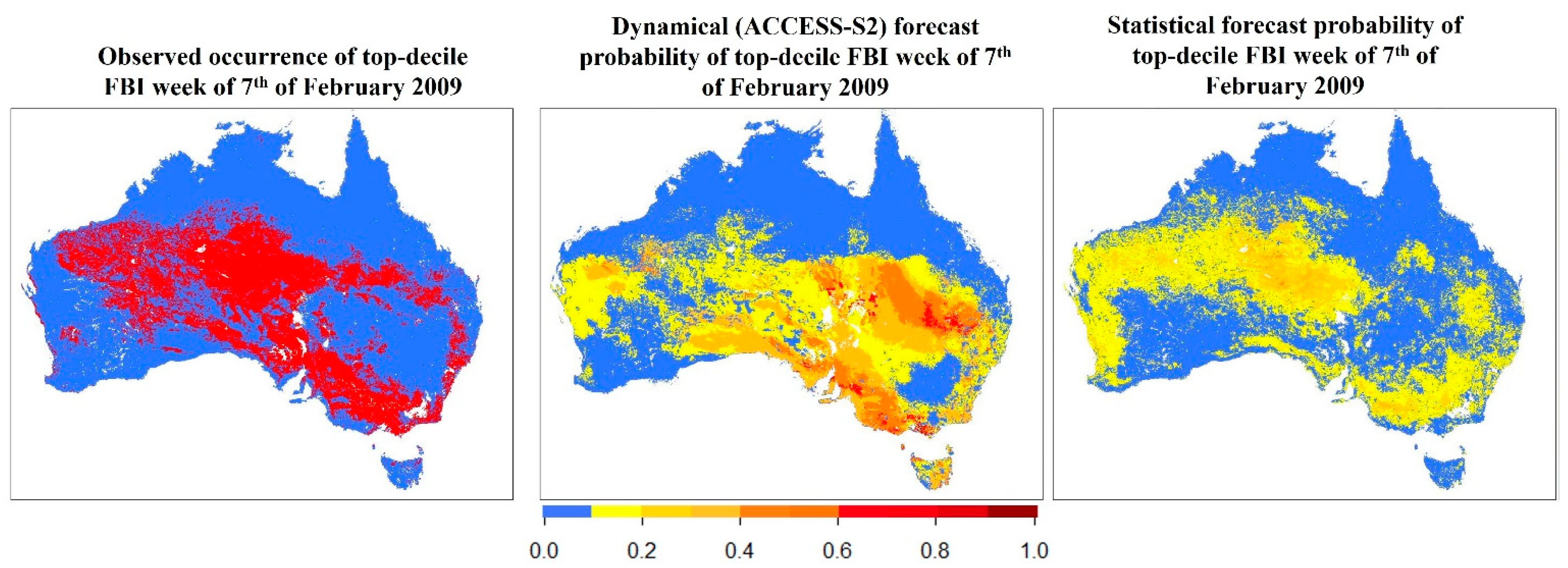
Figure 3. Observed occurrence and forecasted probability of 90th percentile FBI on the week of 7 February 2009.
Atmosphere 15 00470 g003
Figure 4. Contribution of each climate driver to statistical forecast probability of 90th percentile FBI for the week of 7 February 2009 according to linear regression.
Atmosphere 15 00470 g004
Figure 5. Observed occurrence and forecasted probability of 90th percentile FBI for the week of 25 November 2015.
Atmosphere 15 00470 g005
Figure 6. Contribution of each climate driver to statistical forecast probability of 90th percentile FBI for the week of 25 November 2015 according to linear regression.
Atmosphere 15 00470 g006
Table 1. Indices defining climate drivers in an evaluation of their impacts on Australian fire danger.
DriverDriver NameIndexReference Study
MJOMadden Julian OscillationReal-time Multivariate MJO series 1 and 2Wheeler & Hendon, 2004 [48]
ENSOEl Nino Southern OscillationNINO-3.4Trenberth, 1997 [49]
IODIndian Ocean DipoleDipole Mode IndexSaji & Yamagata, 2003 [50]
SAMSouthern Annular ModeAntarctic Oscillation IndexGong & Wang, 1999 [51]
Split-Flow Blocking Blocking IndexPook & Gibson, 1999 [52]
STRHSub-tropical Ridge HighSTRH IndexMarshall et al., 2014 [16]
Table 3. Contingency table, accuracy, probability of detection, and false alarm ratio for dynamical (ACCESS-S2) and statistical models on week of 18 January 2003 over Australia.
Dynamical ModelStatistical Model
ObservedTotal ObservedTotal
YesNo YesNo
ForecastYes22,36842,03064,398ForecastYes46,80789,720136,527
No28,317177,712206,029 No4103131,977136,080
Total 50,685219,742270,427Total 50,910221,697272,607
Accuracy 0.74Accuracy 0.66
Probability of detection0.28Probability of detection0.85
False alarm ratio0.65False alarm ratio0.66
Table 4. Contingency table, accuracy, probability of detection, and false alarm ratio for dynamical (ACCESS-S2) and statistical models on week of 7 February 2009 over Australia.
Dynamical ModelStatistical Model
ObservedTotal ObservedTotal
YesNo YesNo
ForecastYes61,93868,186130,124ForecastYes62,33948,661111,000
No23,426116,877140,303 No23,669137,938161,607
Total 85,364185,063270,427Total 86,008186,599272,607
Accuracy 0.66Accuracy 0.73
Probability of detection0.57Probability of detection0.57
False alarm ratio0.52False alarm ratio0.44
Table 5. Contingency table, accuracy, probability of detection, and false alarm ratio for dynamical (ACCESS-S2) and statistical models on week of 25 November 2015 over Australia.
Dynamical ModelStatistical Model
ObservedTotal ObservedTotal
YesNo YesNo
ForecastYes15,33638,20853,544ForecastYes36,382117,054153,436
No23,529194,415217,944 No2639117,596120,235
Total 38,865232,623271,488Total 39,021234,650273,671
Accuracy 0.77Accuracy 0.56
Probability of Detection0.25Probability of Detection0.87
False Alarm Ratio0.71False Alarm Ratio0.76
Disclaimer/Publisher’s Note: The statements, opinions and data contained in all publications are solely those of the individual author(s) and contributor(s) and not of MDPI and/or the editor(s). MDPI and/or the editor(s) disclaim responsibility for any injury to people or property resulting from any ideas, methods, instructions or products referred to in the content.