
Research on Prediction Model of Particulate Matter in Dalian Street Canyon

Abstract
1. Introduction
2. Methodology
2.1. Prediction Model of Particle Mass Concentrations
2.2. Model Deduction
- Vehicle exhaust was the sole source of pollution in the street canyon.
- Wind speed was uniform in the urban canopy.
- Different canopy heights were distinguished by site coverage and front density .
- The particle mass concentrations above buildings’ roofs were ignored.
- The particle mass concentrations delivered horizontally to the target volume were equal to the pollutant concentrations exported by the target volume.
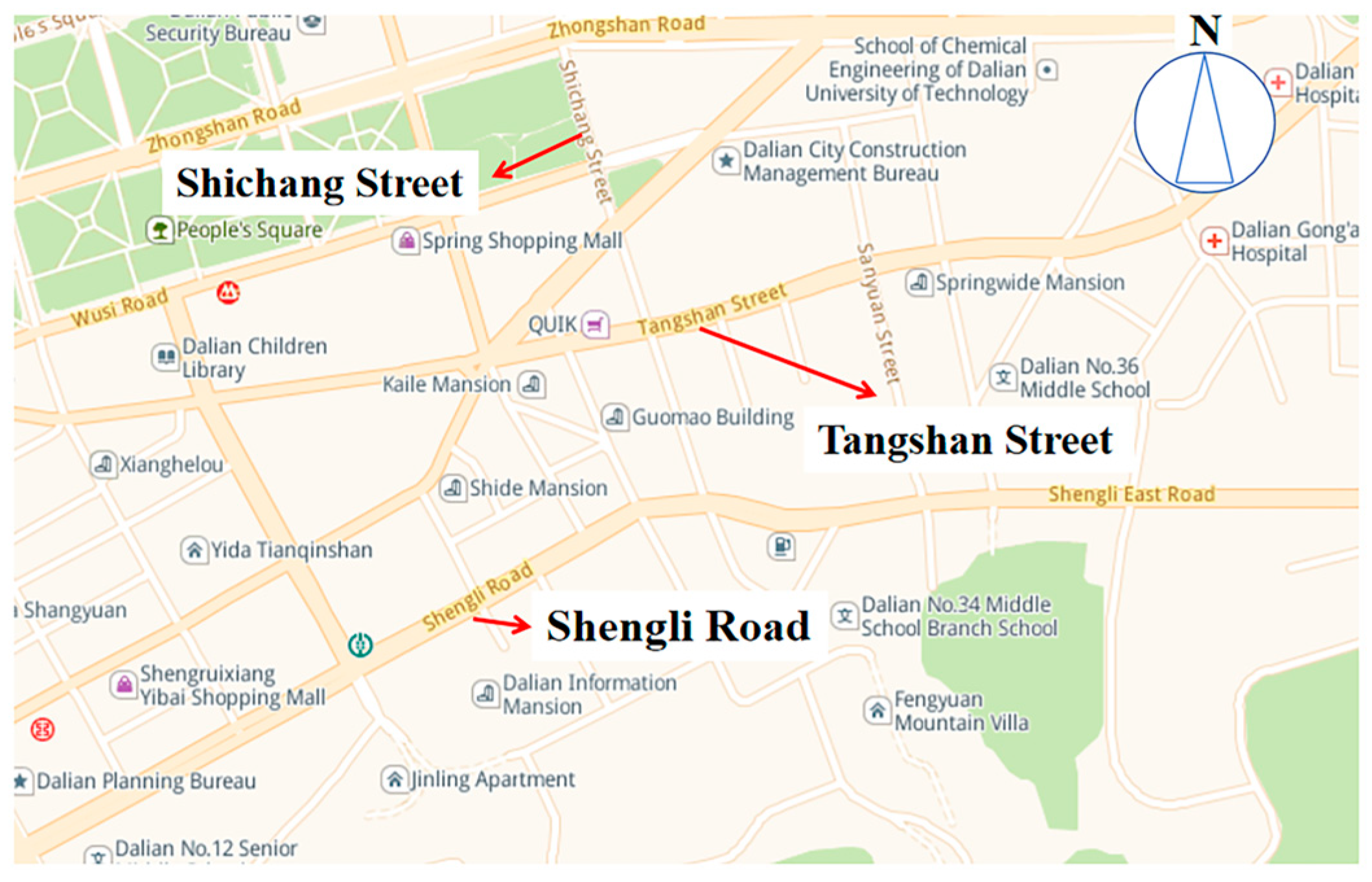
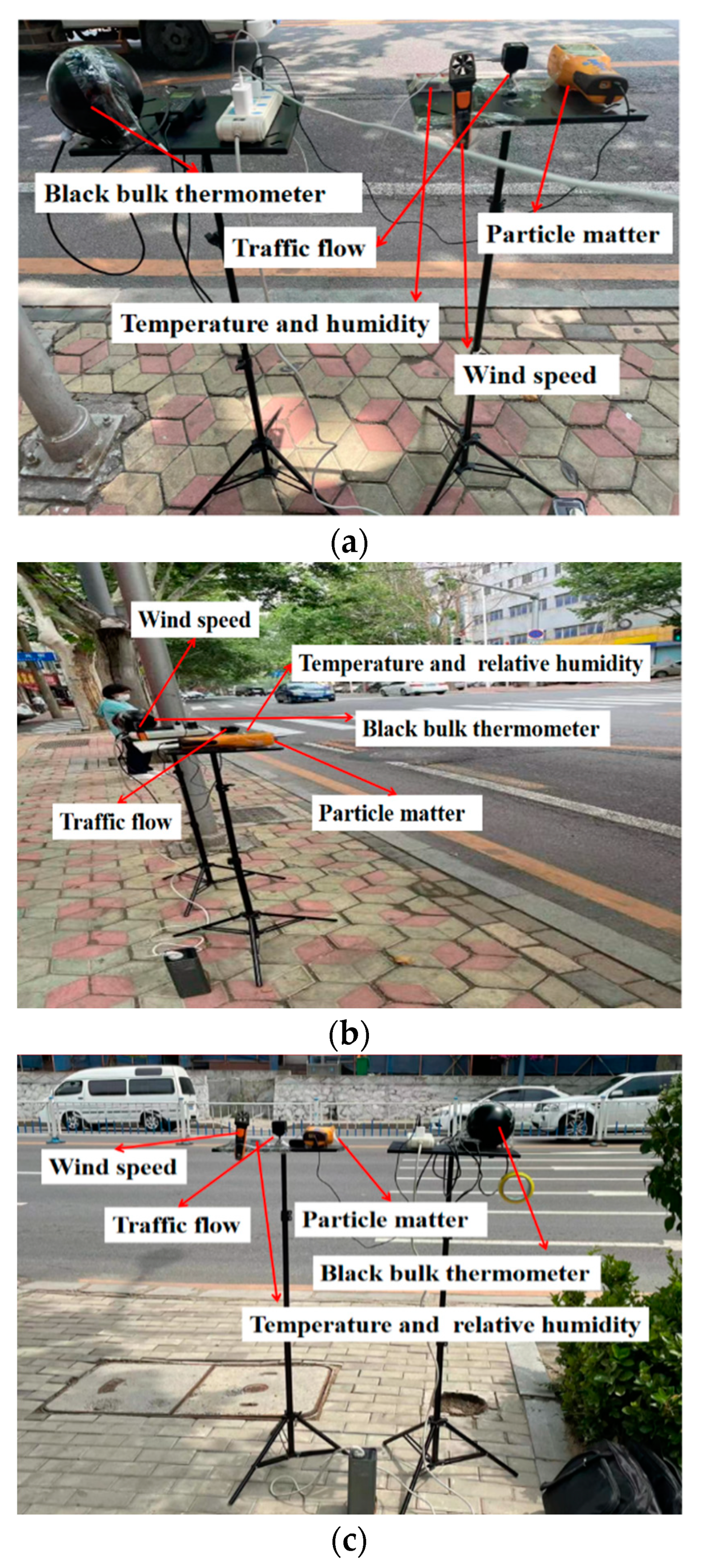
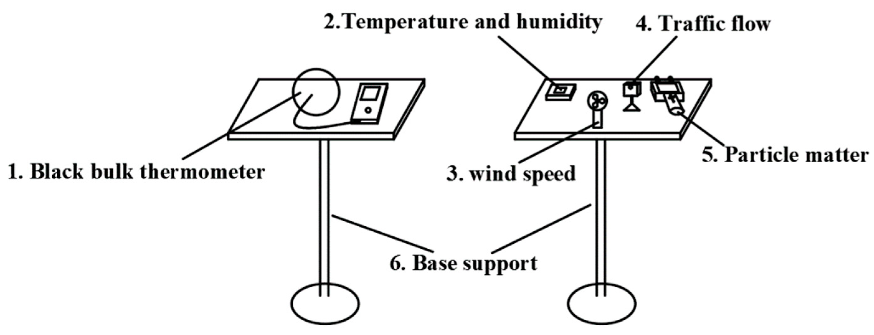
2.3. Field Measurement
2.4. Data Processing
3. Results and Analysis
3.1. Traffic Flow and Meteorological Parameters
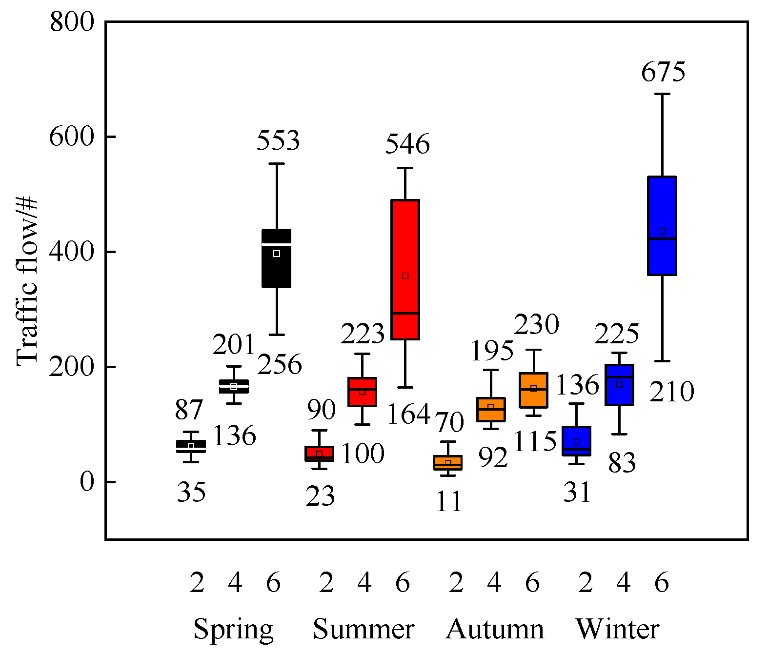
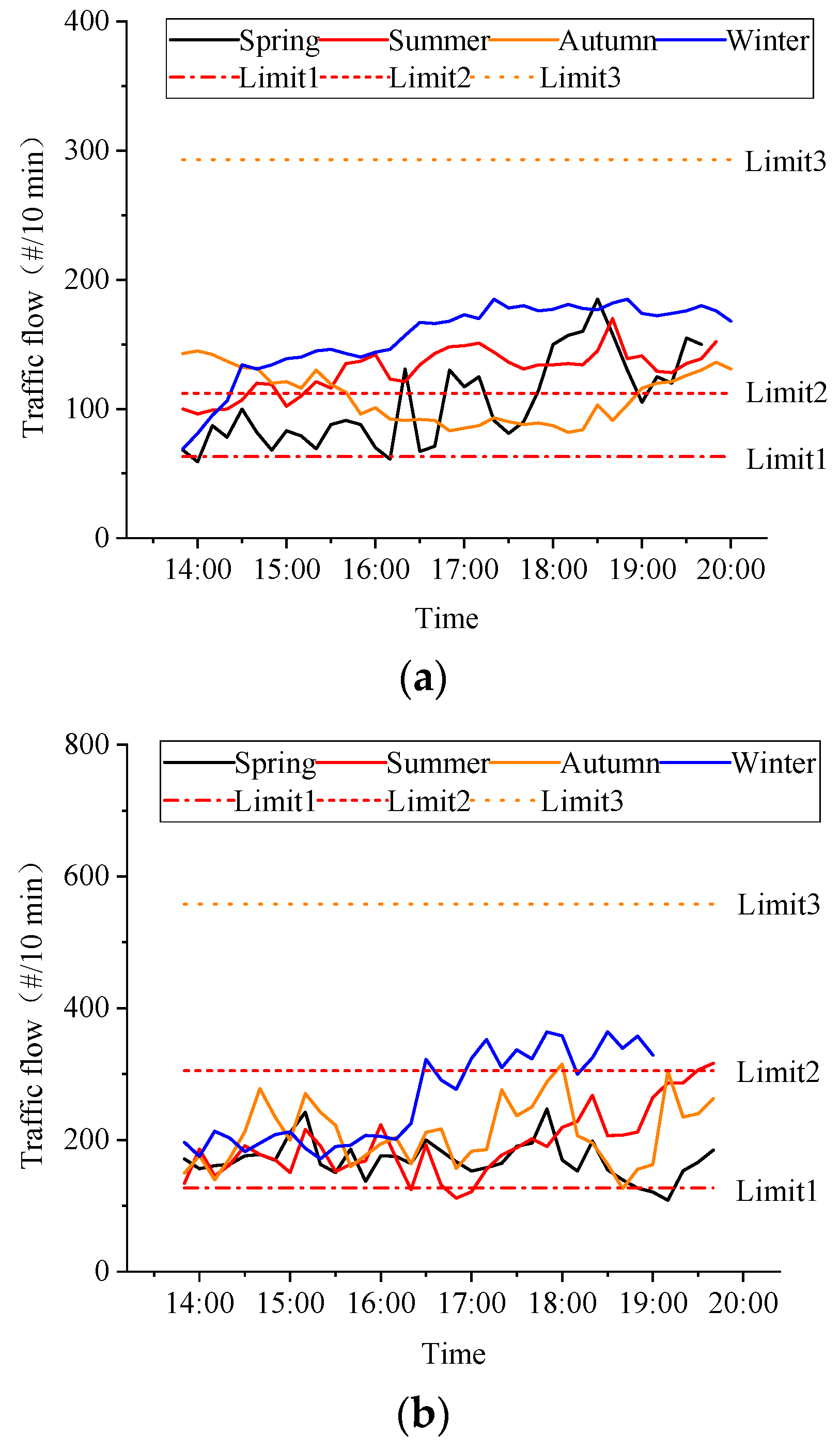
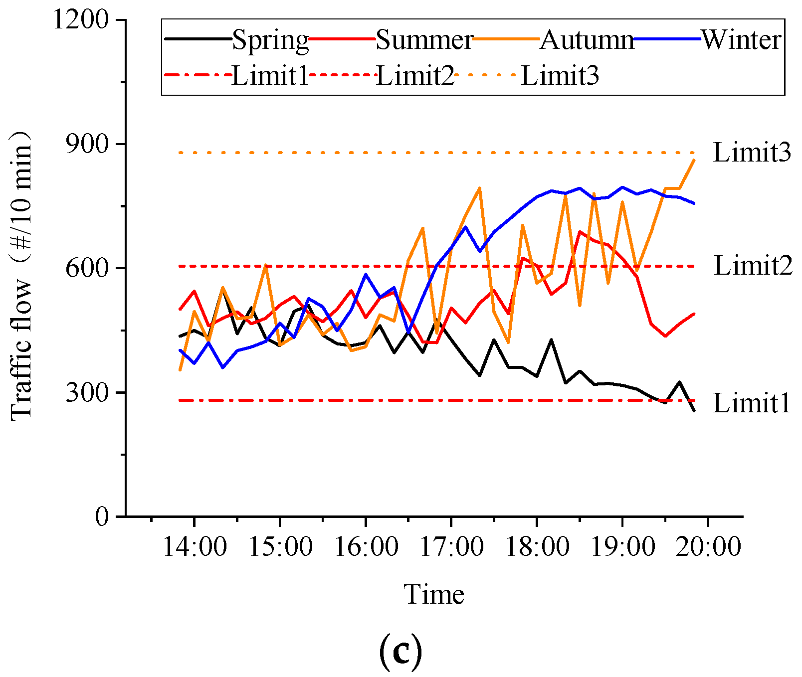
3.1.1. Traffic Flow
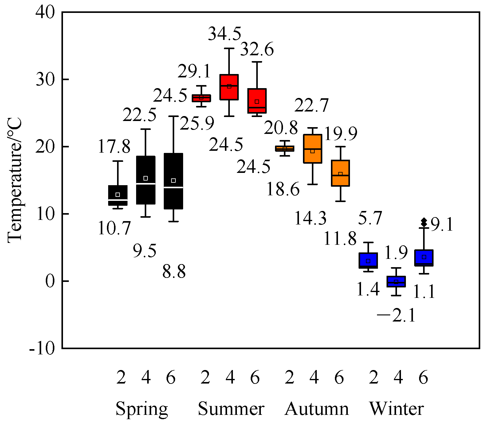
3.1.2. Temperature
3.1.3. Relative Humidity
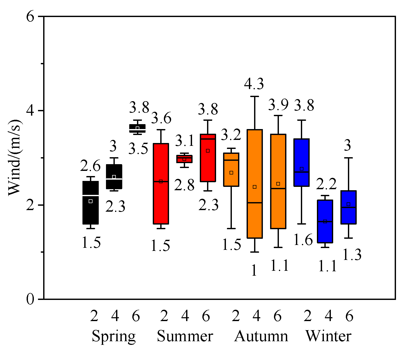
3.1.4. Wind
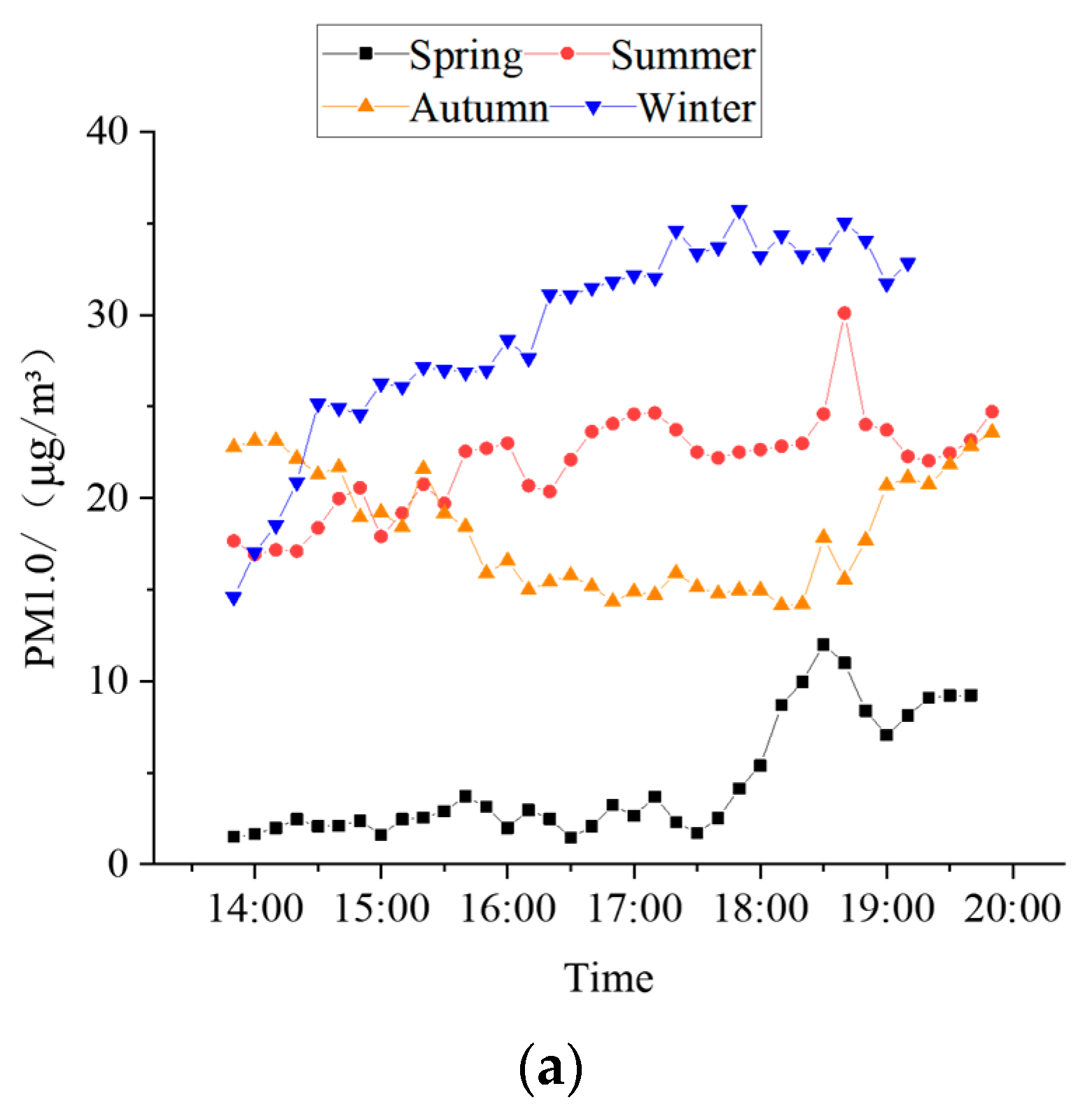
3.1.5. Particulate Matter
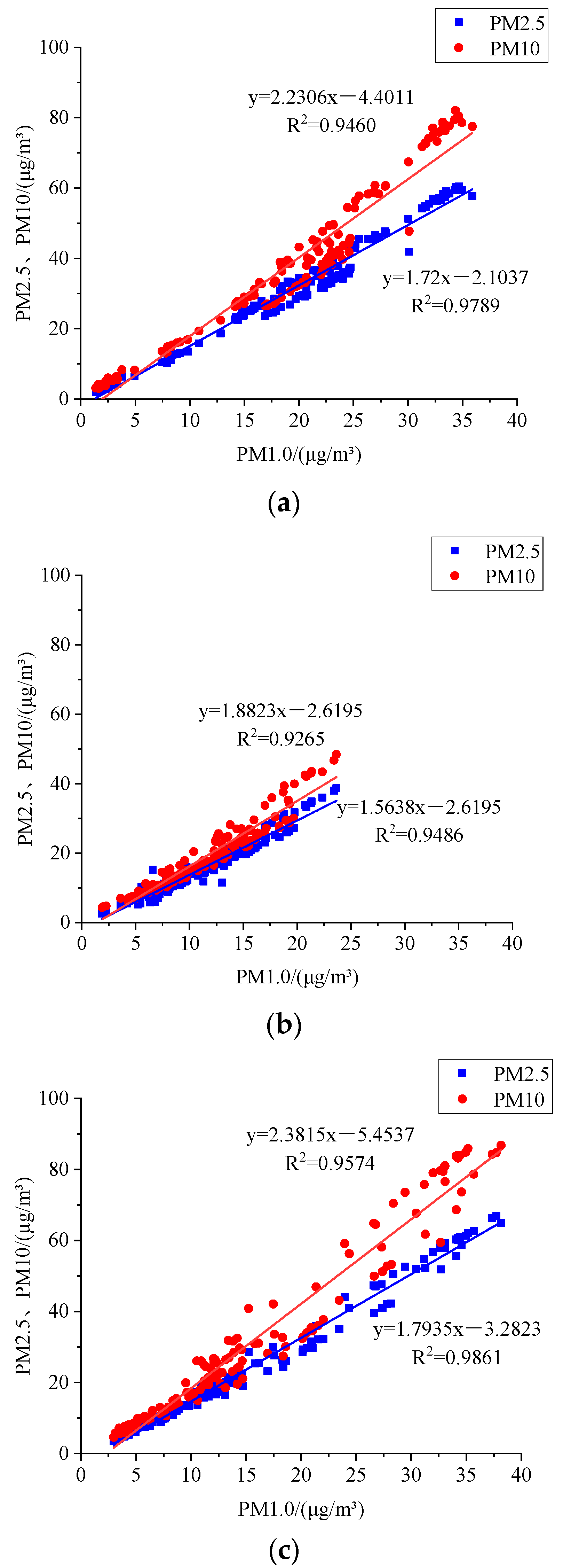
3.2. Analyzing Correlations between PM1.0 and Other Parameters
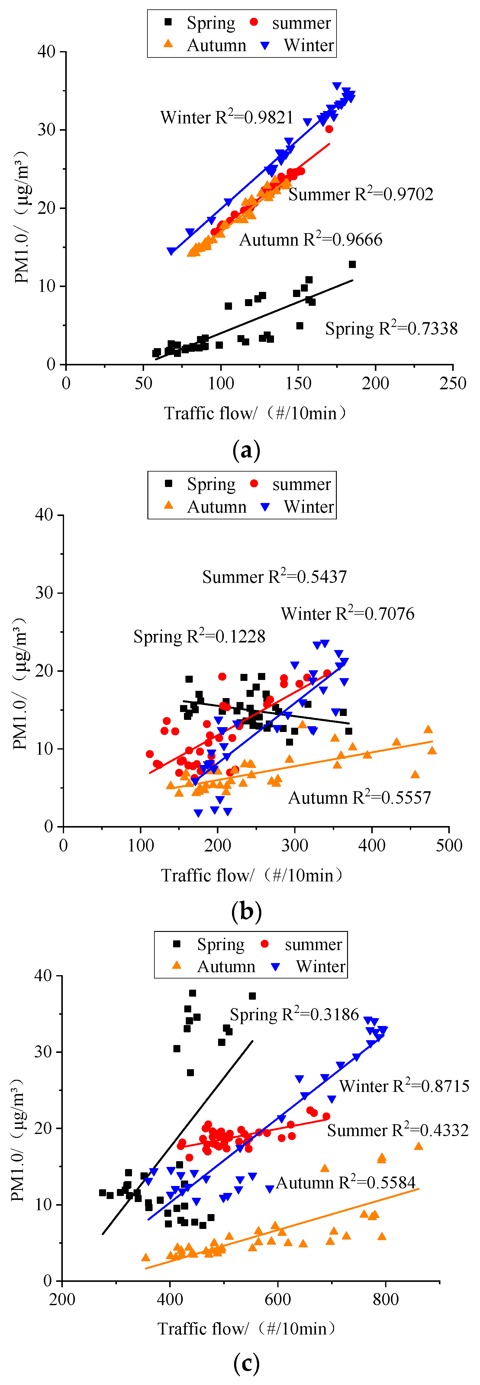
3.2.1. Correlations between Particle Mass Concentrations and Traffic Flow
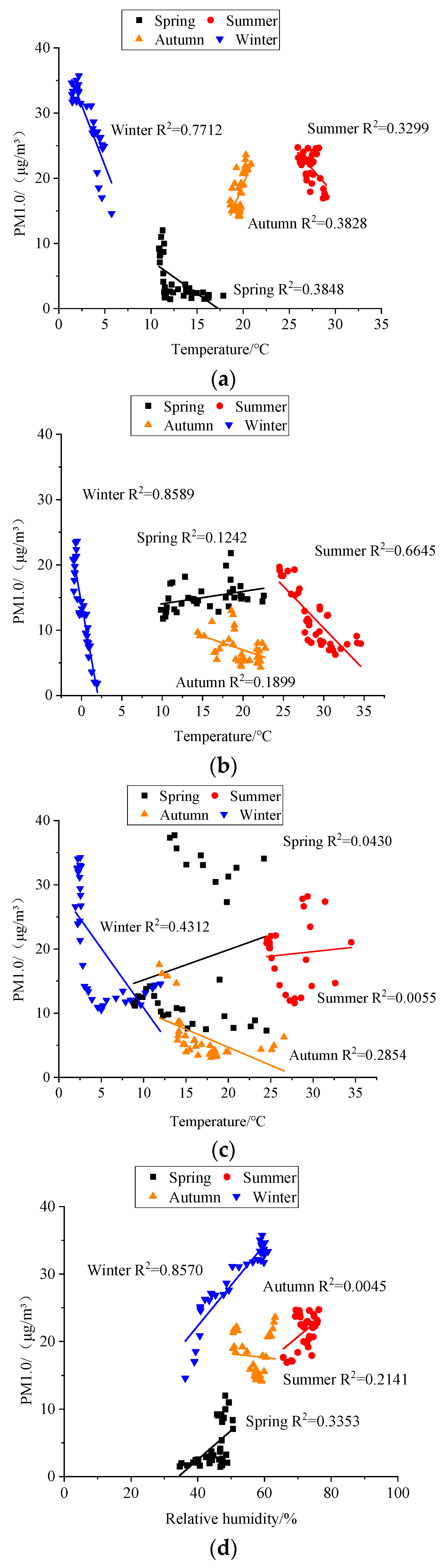
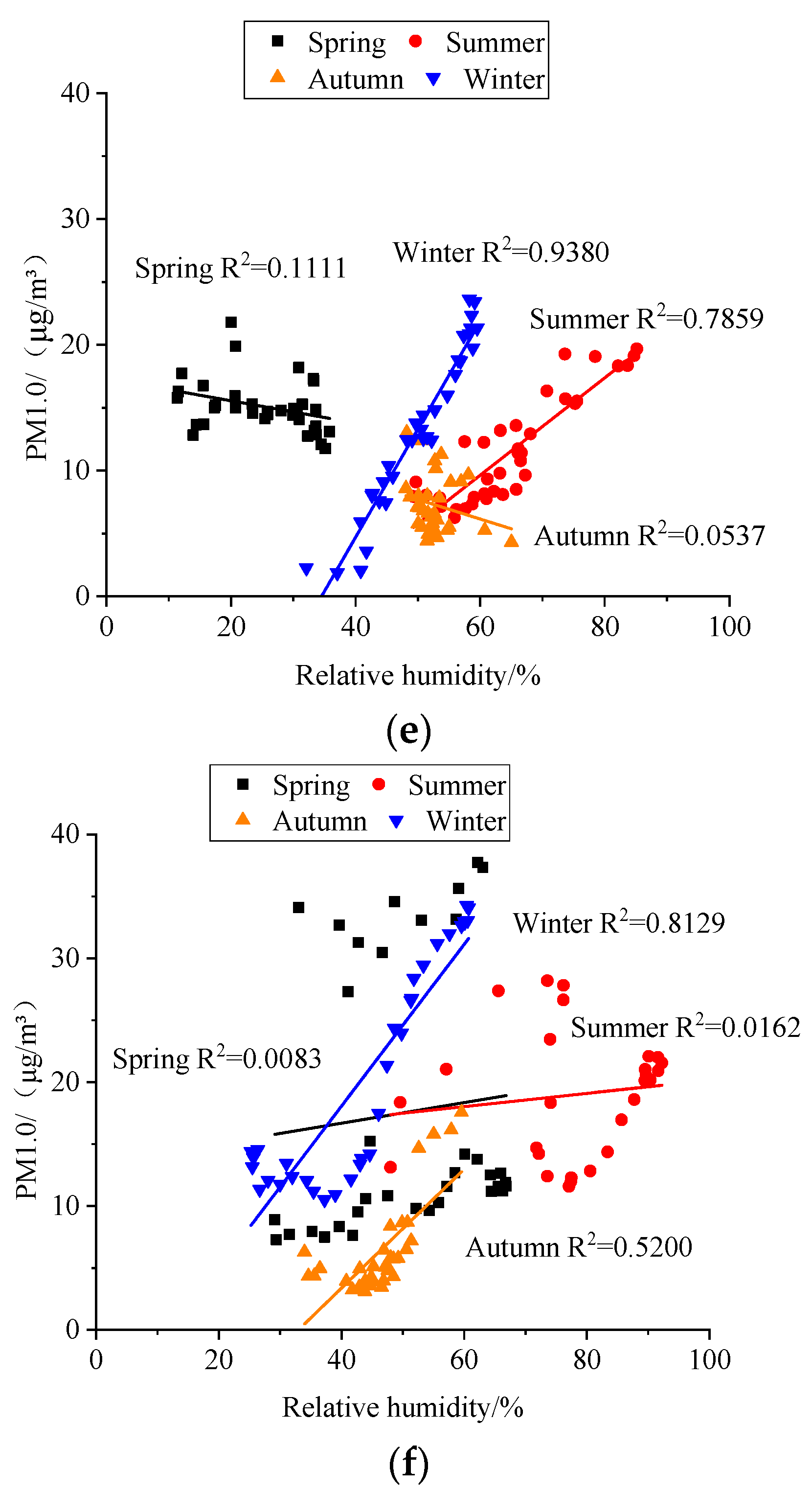
3.2.2. Correlations of Particulate Matter with Temperature and Relative Humidity
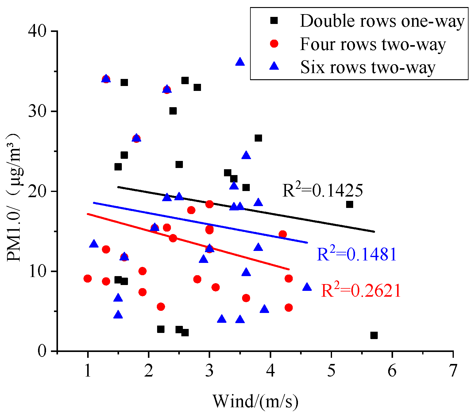
3.2.3. Correlation between Particle Mass Concentrations and Wind
3.3. Model Calculation and Measured Result
3.4. Healthy Environment Analysis for Street Canyon
3.5. Literature Report Comparison
4. Study Limitations
5. Conclusions
- The traffic flow on the three road types exhibited a single-peak distribution. The peak period occurred between approximately 17:30 to 18:30, with approximately 100–150 vehicles/10 min on 2-R, 300–400 vehicles/10 min on 4-R, and 600–700 vehicles/10 min on 6-R.
- PM1.0 mass concentrations measured in the field for 2-R and 4-R were 18.1 ± 10.2 μg/m3 and 16.2 ± 13.1 μg/m3, respectively, which were higher than limit 2 (PM1.0 = 15.8 μg/m3) and lower than limit 3 (PM1.0 = 22.7 μg/m3). Meanwhile, at 4-R, the PM1.0 mass concentration was 11.7 ± 8.43 μg/m3 and it ranged between limit 1 (PM1.0 = 10.2 μg/m3) and limit 2. The PM1.0 mass concentrations at the three road types demonstrated a significant seasonal pattern in winter. The PM1.0 mass concentration showed a positive correlation with traffic flow and relative humidity and a negative correlation with temperature and wind speed.
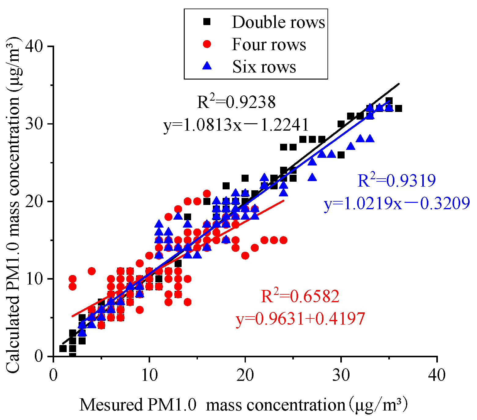
- The prediction model for particle mass concentrations exhibited a high level of accuracy. The prediction step for the PM1.0 mass concentration at 2-R was 14 s, while for 4-R, it was 6 s, and for 6-R, it was 5 s. The correlations between the predicted and measured values for 2-R, 4-R, and 6-R were 0.9319, 0.6582, and 0.9238, respectively.
- The traffic flow of the three road types exceeded limit 1 (recommended by the WHO), with frequencies of 63 for 2-R, 127 for 4-R, and 281 for 6-R. Among the traffic flow exceeding limit 2, 2-R = 112, 4-R = 310, and 6-R = 605. The highest frequency was found on 2-R, followed by 6-R and 4-R. The PM1.0 mass concentration exceeding limit 2 in winter had the longest duration. For other seasons, the traffic flow only exceeded limit 2 during peak hours.
Author Contributions
Funding
Institutional Review Board Statement
Informed Consent Statement
Data Availability Statement
Acknowledgments
Conflicts of Interest
References
- Gurbuz, H.; Sohret, Y.; Ekici, S. Evaluating effects of the COVID-19 pandemic period on energy consumption and enviro-economic indicators of Turkish road transportation. Engery Sources Part A-Recovery Util. Environ. Eff. 2021, 1–13. [Google Scholar] [CrossRef]
- Hudda, N.; Simon, M.; Patton, A.; Durant, J. Reductions in traffic-related black carbon and ultrafine particle number concentrations in an urban neighborhood during the COVID-19 pandemic. Sci. Total Environ. 2020, 2020, 140931. [Google Scholar] [CrossRef]
- Kerimray, A.; Baimatova, N.; Ibragimova, O.; Bukenov, B.; Karaca, F. Assessing airquality changes in large cities during COVID-19 lockdowns: The Impacts of Traffic-free Urban Conditions in Almaty, Kazakhstan. Sci. Total Environ. 2020, 730, 139179. [Google Scholar] [CrossRef]
- Le, V.; Huynh, T.; Olcer, A.; Hoang, A.; Le, A.; Nayak, S.; Pham, V. A remarkable review of the effect of lockdowns during COVID-19 pandemic on global PM emissions. Energy Sources, Part A: Recovery. Util. Environ. Eff. 2020, 2020, 1–16. [Google Scholar] [CrossRef]
- Lian, X.; Huang, J.; Huang, R.; Liu, C.; Wang, L.; Zhang, T. Impact of city lockdown on the air quality of COVID-19-hit of Wuhan city. Sci. Total Environ. 2020, 742, 140556. [Google Scholar] [CrossRef]
- Andronico, D.; Del Carlo, P. PM10 measurements in urban settlements after lava fountain episodes at Mt. Etna, Italy: Pilot test to assess volcanic ash hazard to human health. Nat. Hazards Earth Syst. Sci. 2016, 16, 29–40. [Google Scholar] [CrossRef]
- Di, Q.; Dominici, F.; Schwartz, J.D. Air Pollution and Mortality in the Medicare Population REPLY. N. Engl. J. Med. 2017, 377, 1498–1499. [Google Scholar]
- Dockery, D.W. Acute Respiratory Effects of Particulate Air Pollution. Annu. Rev. Public Health 1994, 15, 107–132. [Google Scholar] [CrossRef]
- Esposito, V.; Lucariello, A.; Savarese, L.; Cinelli, P.; Ferraraccio, F.; Bianco, A.; Luca, D.; Mazzarella, G. Morphology changes in human lung epithelial cells after exposure to diesel exhaust micron sub particles (PM) and pollen allergens. Environ. Pollut. 2012, 171, 162–167. [Google Scholar] [CrossRef]
- Franck, U.; Herbarth, O.; Roder, S.; Schlink, U.; Borte, M.; Diez, U.; Kramer, U.; Lehmann, L. Respiratory effects of indoor particles in young children are size dependent. Sci. Total Environ. 2011, 409, 1621–1631. [Google Scholar] [CrossRef]
- Katsouyanni, K.; Touloumi, G.; Spix, C.; Schwartz, J.; Balducci, F.; Medina, S.; Rossi, G.; Wojtyniak, B.; Sunyer, J.; Bacharova, L.; et al. Short term effects of ambient sulphur dioxide and particulate matter on mortality in 12 European cities: Results from time series data from the APHEA project. BMJ Br. Med. J. 1997, 314, 1658–1663. [Google Scholar] [CrossRef]
- Lim, J.M.; Lee, C.Y.; Lee, Y.; Kim, H.; Lee, J. Characteristics of airborne PM1.0 and associated chemical constituents at a roadside in Korwa. Environ. Eng. Res. 2023, 28, 220089. [Google Scholar] [CrossRef]
- Liu, W.; Du, W.; Wang, J.; Zhuo, S.; Chen, Y.; Lin, N.; Kong, G.; Pan, B. PAHs bound to submicron particles in rural Chinese homes burning solid fuels. Ecotoxicol. Environ. Saf. 2022, 247, 114274. [Google Scholar] [CrossRef]
- Niu, L.; Ye, H.; Xu, C.; Yao, Y.; Liu, W. Highly time- and size-resolved fingerprint analysis and risk assessment of airborne elements in a megacity in the Yangtze River Delta, China. Chemosphere 2015, 119, 112–121. [Google Scholar] [CrossRef]
- Wang, Y.; Kloog, I.; Coull, B.; Kosheleva, A.; Zanobetti, A.; Schwartz, J. Estimating causal effects of long-term PM2.5 exposure on mortality in New Jersey. Environ. Health Perspect. 2016, 124, 1182–1188. [Google Scholar] [CrossRef]
- Yang, T.; Jiang, L.; Bi, X.; Cheng, L.; Zheng, X.; Wang, X.; Zhou, X. Submicron aerosols share potential pathogens and antibiotic resistomes with wastewater or sludge. Sci. Total Environ. 2022, 821, 153521. [Google Scholar] [CrossRef]
- Yang, T.; Jiang, L.; Cheng, L.; Zheng, X.; Bi, X.; Wang, X.; Zhou, X. Characteristics of size-segregated aerosols emitted from an aerobic moving bed biofilm reactor at a full-scale wastewater treatment plant. J. Hazard. Mater. 2021, 416, 125833. [Google Scholar] [CrossRef]
- Zanobetti, A.; Bind, M.A.C.; Schwartz, J. Particulate air pollution and survival in a COPD cohort. Environ. Health 2008, 7, 48. [Google Scholar] [CrossRef]
- Zhao, Y.; Song, X.; Wang, Y.; Zhao, J.; Zhu, K. Seasonal patterns of PM10, PM2.5, and PM1.0 concentrations in a naturally ventilated residential underground garage. Build. Environ. 2017, 124, 294–314. [Google Scholar] [CrossRef]
- Zou, Y.; Wu, Y.; Wang, Y.; Li, Y.; Jin, C. Physicochemical properties, in vitro cytotoxic and genotoxic effects of PM1.0 and PM2.5 from Shanghai, China. Environ. Sci. Pollut. Res. 2017, 24, 19508–19516. [Google Scholar] [CrossRef]
- Kwon, S.; Won, S.; Lim, H.; Hong, S.; Lee, Y.; Jung, J.; Choi, S.; Lee, S.; Oh, S.; Kim, J.; et al. Relationship between PM1.0 and PM2.5 in urban and background areas of Republic of Korea. Atmos. Pollut. Res. 2016, 14, 101858. [Google Scholar] [CrossRef]
- Lee, S.; Cheng, Y.; Ho, K.; Cao, J.; Louie, P.; Chow, J.; Watson, J. PM(1.0) and PM(2.5) Characteristics in the Roadside Environment of Hong Kong. Aerosol Sci. Technol. J. Am. Assoc. Aerosol Res. 2006, 40, 157–165. [Google Scholar] [CrossRef]
- Zhang, Y.; Gu, Z.; Cheng, Y.; Shen, Z.; Dong, J.; Lee, S. Measurement of diurnal variations of PM2.5 mass concentrations and factors affecting pollutant dispersion in urban street canyons under weak-wind conditions in Xi’an. Aerosol Air Qual. Res. 2012, 12, 1261–1268. [Google Scholar] [CrossRef]
- Brook, J.R.; Dann, T.F.; Burnett, R.T. The relationship among TSP, PM10, PM2.5, and inorganic constituents of atmospheric particulate matter at multiple Canadian locations. J. Air Waste Manag. Assoc. 1997, 47, 2–19. [Google Scholar] [CrossRef]
- Dominici, F.; Peng, R.; Bell, M.; Pham, L.; Mc, D.; Zeger, S.; Samet, J. Fine particulate air pollution and hospital admission for cardio vascular and respiratory diseases. J. Am. Med. Assoc. 2006, 295, 1127–1134. [Google Scholar] [CrossRef]
- Giuliano, A.; Gioiella, F.; Sofia, D.; Lotrecchiano, N. A novel methodology and technology to promote the social acceptance of biomass power plants avoiding nimby syndrome. Chem. Eng. Trans. 2018, 67, 307–312. [Google Scholar] [CrossRef]
- Lotrecchiano, N.; Sofia, D.; Giuliano, A.; Barletta, D.; Poletto, M. Real-time On-road Monitoring Network of Air Quality. Chem. Eng. Trans. 2019, 74, 241. [Google Scholar] [CrossRef]
- Sofia, D.; Giuliano, A.; Gioiella, F. Air quality monitoring network for tracking pollutants. the case study ofSalerno city center. Chem. Eng. Trans. 2018, 68, 67–72. [Google Scholar] [CrossRef]
- Dhakal, S.; Gautam, Y.; Bhattarai, A. Exploring a deep LSTM neural network to forecast daily PM2.5 concentration using meteorological parameters in Kathmandu Canyon, Nepal. Air Qual. Atmos. Health 2020, 14, 83–96. [Google Scholar] [CrossRef]
- Alhanafy, T.E.; Zaghlool, F.; Saad, A.; Moustafa, E. Neuro Fuzzy Modeling Scheme for the Prediction of Air Pollution. J. Am. Sci. 2010, 6, 605–616. [Google Scholar]
- Goyal, P.; Chan, A.T.; Jaiswal, N. Statistical models for the prediction of respirable suspended particulate matter in urban cities. Atmos. Environ. 2006, 40, 2068–2077. [Google Scholar] [CrossRef]
- Gupta, P.; Christopher, S.A. Particulate Matter Air Quality Assessment using Integrated Surface, Satellite, and Meteorological Products. J. Geophys. Res. Atmos. 2009, 114. [Google Scholar] [CrossRef]
- Islam, M.M.; Sharmin, M.; Ahmed, F. Predicting air quality of Dhaka and Sylhet divisions in Bangladesh: A time series modeling approach. Air Qual. Atmos. Health 2020, 13, 607–615. [Google Scholar] [CrossRef]
- Loy-Benitez, J.; Vilela, P.; Li, Q.; Yoo, C. Sequential prediction of quantitative health risk assessment for the fine particulate matter in an underground facility using deep recurrent neural networks. Ecotoxicol. Environ. Saf. 2019, 169, 316–324. [Google Scholar] [CrossRef]
- Tong, W.; Li, L.; Zhou, X.; Hamilton, A.; Zhang, K. Deep learning PM2.5 concentrations with bidirectional LSTM RNN. Air Qual. Atmos. Health 2019, 12, 411–423. [Google Scholar] [CrossRef]
- Appel, K.W.; Napelenok, S.L.; Foley, K.M.; Pye, H.O.T.; Hogrefe, C.; Luecken, D.J.; Bash, J.O.; Roselle, S.J.; Pleim, J.E.; Foroutan, H.; et al. Description and evaluation of the Community Multiscale Air Quality (CMAQ) modeling system version 5.1. Geosci. Model Dev. 2017, 10, 1703–1732. [Google Scholar] [CrossRef] [PubMed]
- Mailler, S.; Menut, L.; Khvorostyanov, D.; Valari, M.; Couvidat, F.; Siour, G.; Turquety, S.; Briant, R.; Tuccella, P.; Bessagnet, B.; et al. CHIMERE-2017: From urban to hemispheric chemistry-transport modeling. Geosci. Model Dev. 2017, 10, 2397–2423. [Google Scholar] [CrossRef]
- Tuccella, P.; Curci, G.; Visconti, G.; Bessagnet, B.; Menut, L.; Park, R. Modeling of gas and aerosol with WRF/Chem over Europe: Evaluation and sensitivity study. J. Geophys. Res. Atmos. 2012, 117. [Google Scholar] [CrossRef]
- Finardi, S.; De, M.; D’Allura, A.; Cascone, C.; Calori, G.; Lollobrigida, F. A deterministic air quality forecasting system for Torino urban area, Italy. Environ. Model. Softw. 2008, 23, 344–355. [Google Scholar] [CrossRef]
- Zhao, Y.; Jiang, C.; Song, X.; Li, Z.; Zhang, Y. Modelling particle diffusion patterns inside urban road tunnels in Dalian, China, employing annual field measurement. Build. Environ. 2021, 194, 107681. [Google Scholar] [CrossRef]
- Chianese, E.; Camastra, F.; Ciaramella, A.; Landi, T.; Staiano, A.; Riccio, A. Spatio-temporal learning in predicting ambient particulate matter concentration by multi-layer perceptron. Ecol. Inform. 2018, 49, 54–61. [Google Scholar] [CrossRef]
- Gulia, S.; Nagendra, S.M.S.; Khare, M. A system based approach to develop hybrid model predicting extreme urban NOx and PM2.5 concentrations. Transp. Res. Part D-Transp. Environ. 2017, 56, 141–154. [Google Scholar] [CrossRef]
- Li, R.; Mei, X.; Wei, L.; Han, X.; Zhang, M.; Jing, Y. Study on the contribution of transport to PM2.5 in typical regions of China using the regional air quality model RAMS-CMAQ. Atmos. Environ. 2019, 214, 116856. [Google Scholar] [CrossRef]
- Kusaka, H.; Kimura, F. Coupling a Single-Layer Urban Canopy Model with a Simple Atmospheric Model: Impact on Urban Heat Island Simulation for an Idealized Case. J. Meteorol. Soc. Jpn. 2004, 82, 67–80. [Google Scholar] [CrossRef]
- Krayenhoff, E.S.; Jiang, T.; Christen, A.; Martilli, A.; Oke, T.; Bailey, B.; Nazarian, N.; Voogt, J.; Giometto, M.; Stastny, A. A multi-layer urban canopy meteorological model with trees (BEP- Tree): Street tree impacts on pedestrian-level climate. Urban Clim. 2020, 32, 100590. [Google Scholar] [CrossRef]
- Yuan, C.; Shan, R.; Zhang, Y.; Li, X.; Yin, T.; Hang, J.; Norford, L. Multilayer urban canopy modelling and mapping for traffic pollutant dispersion at high density urban areas. Sci. Total Environ. 2019, 647, 255–267. [Google Scholar] [CrossRef]
- Rakowska, A.; Wong, K.; Townsend, T.; Chan, K.; Westerdahl, D.; Ng, S.; Mocnik, G.; Drinovec, L.; Ning, Z. Impact of traffic volume and composition on the air quality and pedestrian exposure in urban street canyon. Atmos. Environ. 2014, 98, 260–270. [Google Scholar] [CrossRef]
- Kim, T.K. T test as a parametric statistic. Korean J. Anesthesiol. 2015, 68, 540–546. [Google Scholar] [CrossRef]
- Kruschke, J.K. Bayesian estimation supersedes the t test. J. Exp. Psychol. Gen. 2013, 142, 573. [Google Scholar] [CrossRef]
- Ruxton, G.D. The unequal variance t-test is an underused alternative to Student’s t-test and the Mann–Whitney U test. Behav. Ecol. 2010, 17, 688–690. [Google Scholar] [CrossRef]
- Xu, M.; Fralick, D.; Zheng, J.; Wang, B.; Tu, X.; Feng, C. The differences and similarities between two-sample t-test and paired t-test. Shanghai Arch. Psychiatry 2017, 29, 184–188. [Google Scholar] [CrossRef]
- Megaritis, A.; Fountoukis, C.; Charalampidis, P.; Pilinis, C.; Pandis, S. Response of fine particulate matter concentrations to changes of emissions and temperature in Europe. Atmos. Chem. Phys. 2013, 13, 3423–3443. [Google Scholar] [CrossRef]
- Galindo, N.; Varea, M.; Gil-Molto, J.; Yubero, E.; Nicolas, J. The Influence of Meteorology on Particulate Matter Concentrations at an Urban Mediterranean Location. Water Air Soil Pollut. 2011, 215, 365–372. [Google Scholar] [CrossRef]
- Zhang, B.; Jiao, L.; Xu, G.; Zhao, S.; Tang, X.; Zhou, Y.; Gong, C. Influences of wind and precipitation on different-sized particulate matter concentrations (PM2.5, PM10, PM2.5–10). Meteorol. Atmos. Phys. 2017, 130, 383–392. [Google Scholar] [CrossRef]
- Chen, C.; Zhang, H.; Li, H.; Wu, N.; Zhang, Q. Chemical characteristics and source apportionment of ambient PM1.0 and PM2.5 in a polluted city in North China plain. Atmos. Environ. 2020, 242, 117867. [Google Scholar] [CrossRef]
- Han, J.; Lim, S.; Meehye, L.; Lee, Y.; Woong, L.; Shim, C.; Chang, L. Characterization of PM2.5 Mass in Relation to PM1.0 and PM10 in Megacity Seoul. Asian J. Atmos. Environ. 2022, 16, 2021124. [Google Scholar] [CrossRef]
- Li, Y.; Chen, Q.; Zhao, H.; Wang, L.; Tao, R. Variations in PM10, PM2.5 and PM10 in an Urban Area of the Sichuan Basin and Their relation to meteorological factors. Atmosphere 2015, 6, 150–163. [Google Scholar] [CrossRef]
- World Health Organization. WHO Global Air Quality Guidelines: Particulate Matter (PM2.5 and PM10), Ozone, Nitrogen Dioxide, Sulfur Dioxide and Carbon Monoxide; WHO: Geneva, Switzerland, 2021. [Google Scholar]
- Rovelli, S.; Cattaneo, A.; Borghi, F.; Spinazze, A.; Campagnolo, D.; Limbeck, A.; Cavallo, D. Mass Concentration and Size-Distribution of Atmospheric Particulate Matter in an Urban Environment. Aerosol Air Qual. Res. 2016, 17, 1142–1155. [Google Scholar] [CrossRef]
- Shindler, L. Development of a low-cost sensing platform for air quality monitoring: Application in the city of Rome. Environ. Technol. 2019, 2019, 1–14. [Google Scholar] [CrossRef]


| Instrument | Range | Resolution | Accuracy |
|---|---|---|---|
| 179 dt DTH temperature and humidity recorder | 0–80 °C | 0.01 °C | ±0.4 °C |
| 0–100% | 0.01% | ±3% | |
| Korno GT-1000 composite pollutant mass | 0–500 µg/m3 | 1 µg/m3 | ≤±3% |
| concentration detector | |||
| Testo 410i | 0.4~30 m/s | 0.1 m/s | 0.1 m/s |
| Model Parameter | Value |
|---|---|
| Pollutant discharge flux | 4.5 × 10⁻⁶ kg/s/m2 |
| Traffic flow | 10–60 #/min |
| Wind | 1–6 m/s |
| Wind direction | 0–360° |
| Speed | 40–50 km/h |
| Exhaust emission velocity | 0.8 m/s |
| Exhaust port area | 0.02 m2 |
| Long and wide (double rows) | 330 and 5 m |
| Long and wide (four rows) | 320 m and 13 m |
| Long and wide (six rows) | 450 m and 21 m |
| Street canyon canopy height | 3 m |
| Long, wide, and high (car) | 4.6 m, 1.8 m, and 1.5 m |
| External concentration of traffic wind | Measured acquisition |
| Natural wind external concentration | Obtained by China Weather Network |
| 0.05 m/s | |
| 0.43 | |
| 0.0015 | |
| Climate statistics acquisition |
| Road Type | Model |
|---|---|
| 2-R | |
| 4-R | |
| 6-R |
| Grade | PM2.5 | PM1.0 | 2-R | 4-R | 6-R | Non-Accidental Mortality | Level |
|---|---|---|---|---|---|---|---|
| Recommended | 15.0 μg/m3 | 10.2 μg/m3 | 63# | 127# | 281# | 0 | Limit 1 |
| Interim target 4 | 25.0 μg/m3 | 15.8 μg/m3 | 112# | 310# | 605# | 0.7% | Limit 2 |
| Interim target 3 | 37.5 μg/m3 | 22.7 μg/m3 | 293# | 558# | 879# | 1.3% | Limit 3 |
| Interim target 2 | 50.0 μg/m3 | 29.7 μg/m3 | 417# | 1150# | 2200# | 2.3% | Limit 4 |
| Interim target 1 | 75.0 μg/m3 | 43.6 μg/m3 | 870# | 2650# | 3030# | 3.9% | Limit 5 |
Disclaimer/Publisher’s Note: The statements, opinions and data contained in all publications are solely those of the individual author(s) and contributor(s) and not of MDPI and/or the editor(s). MDPI and/or the editor(s) disclaim responsibility for any injury to people or property resulting from any ideas, methods, instructions or products referred to in the content. |
© 2024 by the authors. Licensee MDPI, Basel, Switzerland. This article is an open access article distributed under the terms and conditions of the Creative Commons Attribution (CC BY) license (https://creativecommons.org/licenses/by/4.0/).
Share and Cite
Song, X.; He, Y.; Zhang, Y.; Zhang, G.; Zhou, K.; Que, J. Research on Prediction Model of Particulate Matter in Dalian Street Canyon. Atmosphere 2024, 15, 397. https://doi.org/10.3390/atmos15040397
Song X, He Y, Zhang Y, Zhang G, Zhou K, Que J. Research on Prediction Model of Particulate Matter in Dalian Street Canyon. Atmosphere. 2024; 15(4):397. https://doi.org/10.3390/atmos15040397
Chicago/Turabian StyleSong, Xiaocheng, Yuehui He, Yao Zhang, Guoxin Zhang, Kai Zhou, and Jinhua Que. 2024. "Research on Prediction Model of Particulate Matter in Dalian Street Canyon" Atmosphere 15, no. 4: 397. https://doi.org/10.3390/atmos15040397
APA StyleSong, X., He, Y., Zhang, Y., Zhang, G., Zhou, K., & Que, J. (2024). Research on Prediction Model of Particulate Matter in Dalian Street Canyon. Atmosphere, 15(4), 397. https://doi.org/10.3390/atmos15040397