Defining Detection Limits for Continuous Monitoring Systems for Methane Emissions at Oil and Gas Facilities

Abstract

Networks of fixed-point continuous monitoring systems are becoming widely used in the detection and quantification of methane emissions from oil and gas facilities in the United States. Regulatory agencies and operators are developing performance metrics for these systems, such as minimum detection limits. Performance characteristics, such as minimum detection limits, would ideally be expressed in emission rate units; however, performance parameters such as detection limits for a continuous monitoring system (CMS) will depend on meteorological conditions, the characteristics of emissions at the site where the CMS is deployed, the positioning of CMS devices in relation to the emission sources, and the amount of time allowed for the CMS to detect an emission source. This means that certifying the performance of a CMS will require test protocols with well-defined emission rates and durations; initial protocols are now being used in field tests. Field testing results will vary, however, depending on meteorological conditions and the time allowed for detection. This work demonstrates methods for evaluating CMS performance characteristics using dispersion modeling and defines an approach for normalizing test results to standard meteorological conditions using dispersion modeling.

1. Introduction

Global energy systems have estimated releases of ~100 Tg/y of methane emissions, which have the warming equivalent, over a 20-year period, of >8 Gt/y of carbon dioxide emissions [1]. Extensive analyses and measurement campaigns over the last decade have led to the understanding that emissions from oil and gas facilities consist of both small numbers of large emission events and large numbers of smaller-emission-rate sources [2,3]. Large-emission-rate and short-duration emission events are often attributed to equipment malfunctions [4] and substantial emission reductions are possible if these emissions can be rapidly identified and mitigated. Programs such as the Methane Alert and Response System (MARS), launched by the United Nations Environment Program’s International Methane Emissions Observatory (IMEO), seeks to use remote sensing data to identify large emission events and communicate event detections to operators [5]. In addition, the United States has launched, as part of its data center for greenhouse gas emissions, a program to identify large emission events [6].

While many scientific reports and government programs have used satellite and other remote sensing systems to detect large emission events [7,8], satellite detection methods that have global coverage generally have detection limits > 1000 kg/h, and satellite systems with lower detection limits (hundreds of kg/h) generally have limited spatial coverage. This has led to interest in relatively sparse networks of continuous monitors that can be used to identify large emissions events quickly and to characterize the duration of those events [9,10]. Sparse networks of continuous monitoring systems could be used to achieve the very rapid detection of large emission events.

In addition to using measurements to detect large emission events, there has also been significant interest in using measurements to improve emission quantification and reporting. For example, the United Nations’ Oil and Gas Methane Partnership 2.0 (OGMP 2.0) requires building emission inventories that include measurement and reconciliation [11], and involves over 130 companies with operations in more than 70 countries globally [12]. In the United States, the Environmental Protection Agency (EPA) proposed changes to current emissions reporting that incorporate a greater focus on emission measurements [13]. The requirements for measurement systems that are to be used for emissions reporting differ from the requirements for large-emission-event detection. For emissions reporting, emissions from sources with both large and small emission rates must be detected, measured, and quantified. Because significant fractions of total methane emissions at oil and gas facilities are due to both small numbers of large emission events found at sites with total emission rates that are in the 99th percentile of measurements and large numbers of smaller-emission-rate sources found at virtually all sites, measurement systems must have relatively low detection limits to enable accurate emission reporting.

The need for measurement systems able to detect both small and large emission rate sources has driven the widespread deployment of continuous monitoring networks of fixed-point sensors. The primary advantage of continuous monitoring systems located in close proximity to emission sources is their ability to rapidly detect relatively low emission rates. The U.S. Environmental Protection Agency has established a minimum detection limit (MDL) for continuous monitoring systems (CMSs) for methane emissions in its recent OOOOb/c regulations [14]. That MDL is specified as 0.4 kg/h; however, because continuous monitoring systems do not directly measure emission rate, the detection limit of a CMS is more accurately specified as a concentration enhancement, detectable within a specified period of time. Converting between MDLs based on an emission rate from a source that is remote from a sensor and the concentration enhancement present at the sensor and the time to detection requires assumptions regarding meteorological conditions, the characteristics of emissions at the site, and the positioning of CMS devices in relation to the emission sources. An MDL based on emission rate is application- and time-period specific. This work uses dispersion modeling to develop robust detection limit definitions for CMSs and compares these results based on simulations to controlled release testing results for CMS devices. Based on these analyses, recommendations are made for assessing the MDLs of continuous monitoring systems for methane emissions and how dispersion models can be used to adjust the results to standard sets of meteorological conditions.

2. Methods

2.1. Source and Sensor Configurations

The dispersion modeling performed in this work is based on analyses initially described by Chen et al. [15] In that work, the ability of CMS devices to detect a single idealized source was evaluated by considering a steady emission released at a height of 5.5 m above ground level (agl). The analyses evaluated the ability of CMS devices arrayed in a rectangular grid to detect the emission source. The rectangular grid was used to assess the number of sensors that would need to be deployed at the perimeter of a rectangular oil and gas production pad in order to achieve a targeted efficiency of emission event detection. In this work, the goal is to characterize how the distance from an emission source will influence emission detection. The CMS deployment formed a radial pattern of concentric rings, as shown in Figure 1. In a base-case scenario, CMS devices are deployed radially in concentric rings every 45 degrees, at 10 m, 20 m, 30 m, 40 m, and 50 m from a source that emits at the EPA-defined emission threshold of 0.4 kg/h at a release height of 2.4 m. Sensors were assumed to be located at 2.4 m agl. Simulations were also performed at emission release heights of 5.5 m, which is representative of an emission release from the top of a storage tank.

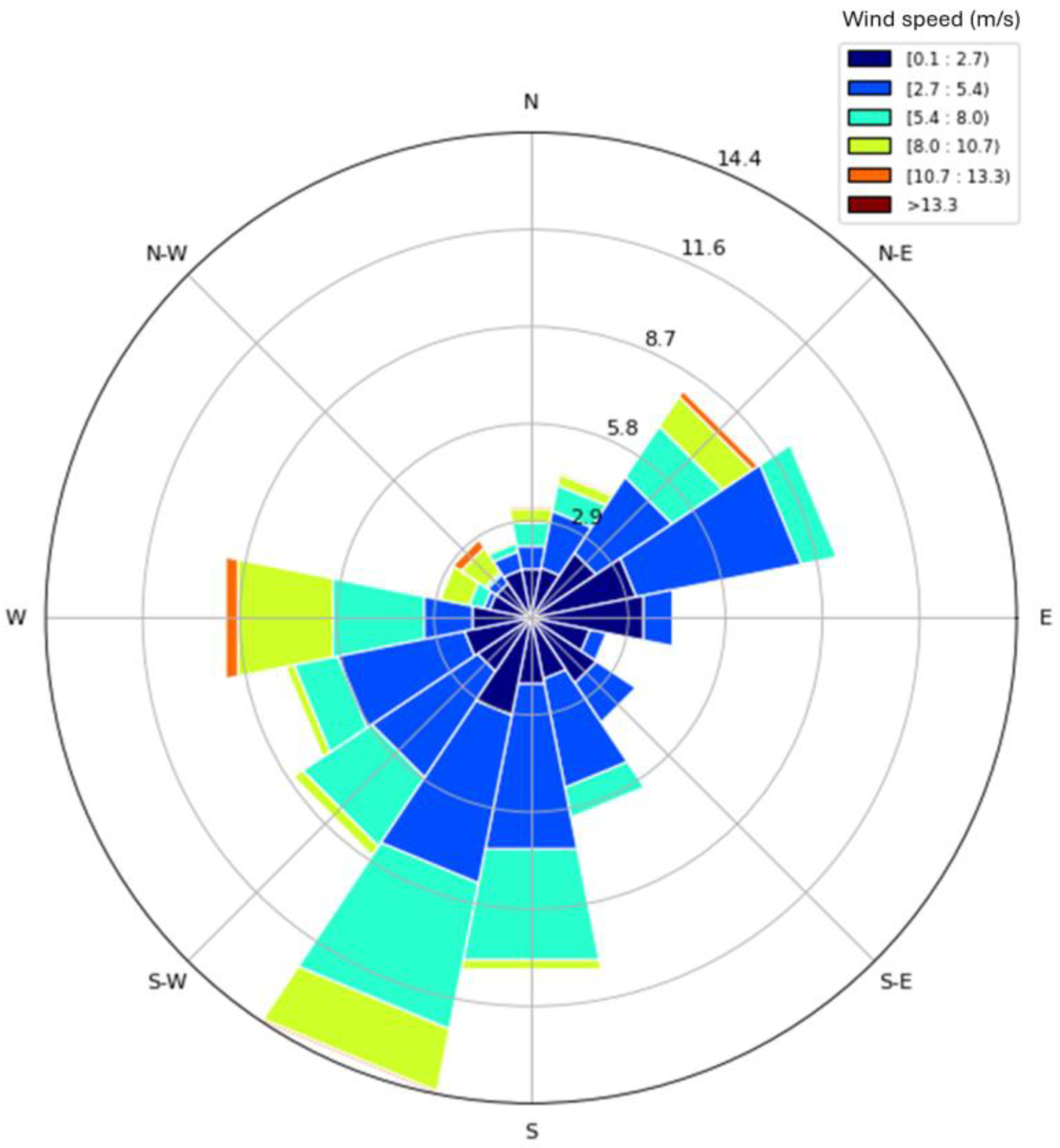
2.2. Dispersion Modeling

Dispersion modeling was performed at a one-minute temporal resolution. A two-week period, chosen to be representative of annual average wind speeds and directions in the Permian Basin in west Texas, was used in the analyses. The Permian Basin is one of the largest oil and gas production regions in the world [16]. A wind rose, summarizing wind speeds and directions during the episode period, is shown in Figure 2. Chen et al. [15] compared the details of the episode period to decadal meteorological data in the region and performed sensitivity analyses on meteorological conditions.

A demonstration network of CMS devices has been operated in a roughly 10 km² region since 2022, encompassing approximately 50 oil and gas production sites and 70 wells in the Permian Basin [17]. Data from six on-site meteorological stations from this network were used to retrieve pressure, temperature, humidity, wind speed, and wind direction observations used in the dispersion model. These data were supplemented by data from National Weather Service stations, twice-daily observations from the National Oceanic and Atmospheric Administration radiosondes, and other information [15].

Dispersion modeling was performed using CALPUFF v7.2.17. Meteorological modeling inputs were generated using CALMET v6.5 [18]. Receptor sites for the modeling included both the sensor locations shown in Figure 1 and a grid with 100 m horizontal spatial resolution with 10 vertical layers. The dispersion model generated methane concentration enhancements as a function of time and spatial locations.

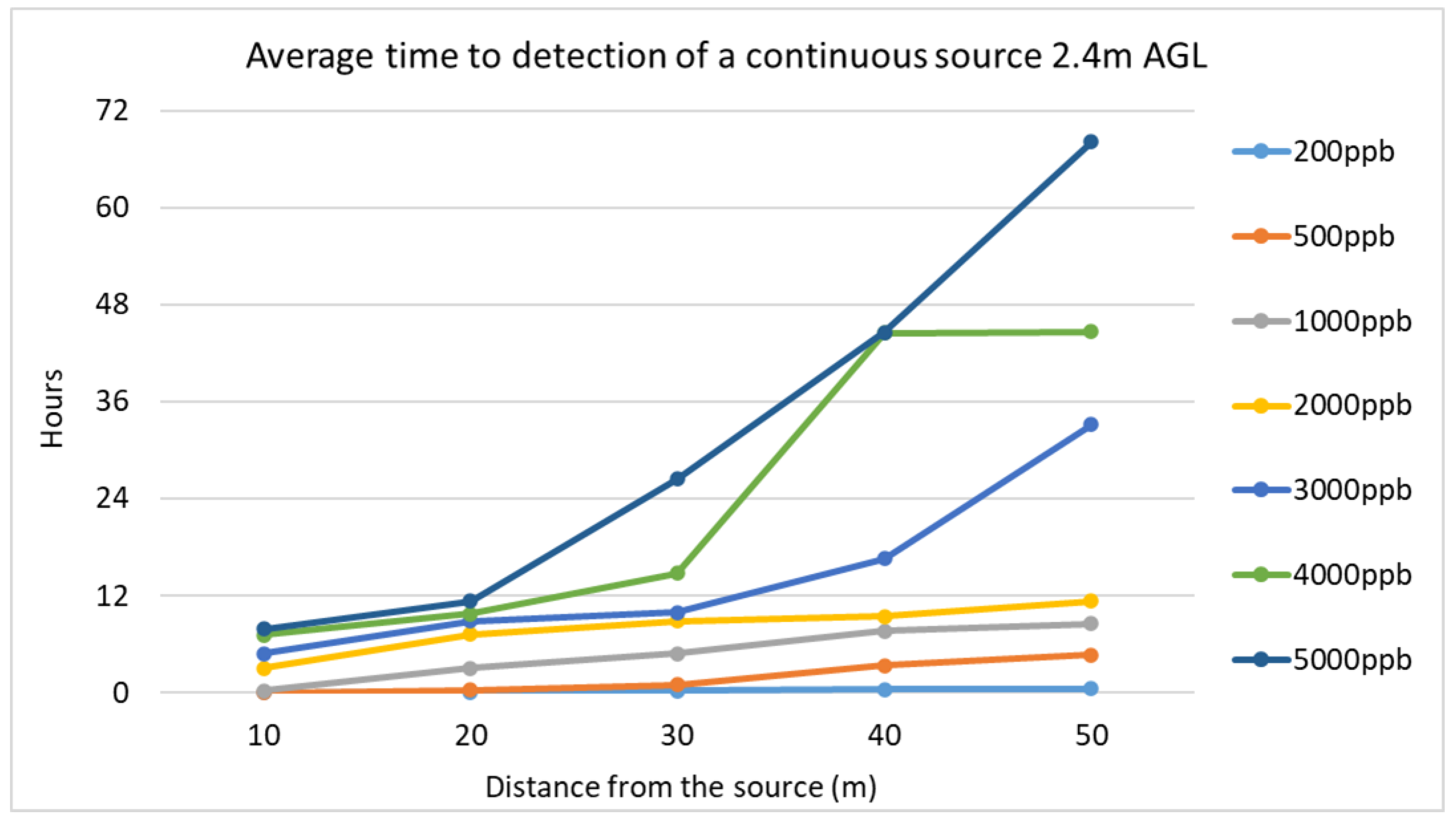
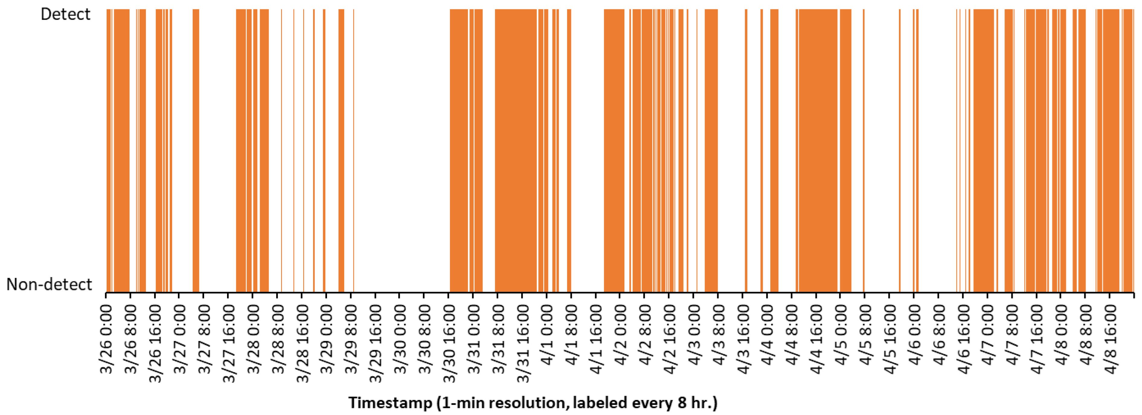
2.3. Event Detection, Temporal Coverage, and Time to Detection

Methane concentration enhancements were simulated for sensors positioned 2.4 m agl in various directions and at various distances from an emission source, as shown in Figure 1. The source was assumed to be emitting methane continuously. An event was assumed to be detected if a one-minute average concentration enhancement exceeded specific concentration thresholds. Thresholds ranging from 200 ppb to 5000 ppb (parts per billion by volume) were considered and were consistent with the range of detection limits covered by commercial methane sensors commonly deployed in the field [19]. The data were summarized in a time series plot, identifying periods of detection and non-detection for single sensors or groups of sensors. Figure 3 shows a time series of periods of detection and non-detection for a group of 8 sensors located 20 m from a source with a release rate of 0.4 kg/s and a release height of 2.4 m agl. Sensors were spaced every 45 degrees, as shown in Figure 1, and a detection threshold of 1 ppm was assumed. In this case, the group of 8 sensors collectively detected an emission event of 0.4 kg/h, 21% of the time.

Emission events were initiated every minute from the start of the two-week period until the last minute that met the event detection criteria (1 min concentration enhancement exceeding the threshold level). Each event was continued until it reached a minute in which a sensor would detect it, based on detection criteria, and the time to detection per event and average times to detection were determined.

3. Results and Discussion

The dispersion modeling simulations were used to generate mappings of the temporal coverage for various sensor configurations. Figure 3 shows the fraction of time in which a 0.4 kg/h emission source with a release point located 2.4 m agl would be observed by at least one of eight sensors deployed every 45 degrees, at 20 m from the source, if the detection threshold was set at 1000 ppb. Similar time series were developed for multiple distances and detection thresholds. As shown in Figure 4, the temporal coverage depends on the concentration enhancement detectable by the sensing system and the distance from the source. At a 10 m distance from the source, a sensing system able to detect a methane concentration enhancement of 2 ppm would detect emissions only about a quarter of the time, while a system capable of detecting a 200 ppb enhancement would detect emissions nearly all of the time.

If effectiveness is defined as a temporal coverage greater than 25%, then only systems with sensors placed every 45 degrees, with a detection threshold of 2 ppm or lower, at a 10 m distance from the source, would be effective. If, however, effectiveness is defined using a time-to-detection metric, and effectiveness is defined as an average time to detection of 12 h or less, then, as shown in Figure 5, systems with sensors placed every 45 degrees, with a wide range of detection thresholds up to 5 ppm, could be effective at a 20 m distance from the source. As shown in Figure 5, with lower detection limits (concentration enhancement threshold < 2 ppm), time to detection is more sensitive to detection thresholds than the distance from the source. Systems with sensors separated by more than 45 degrees could also be effective.

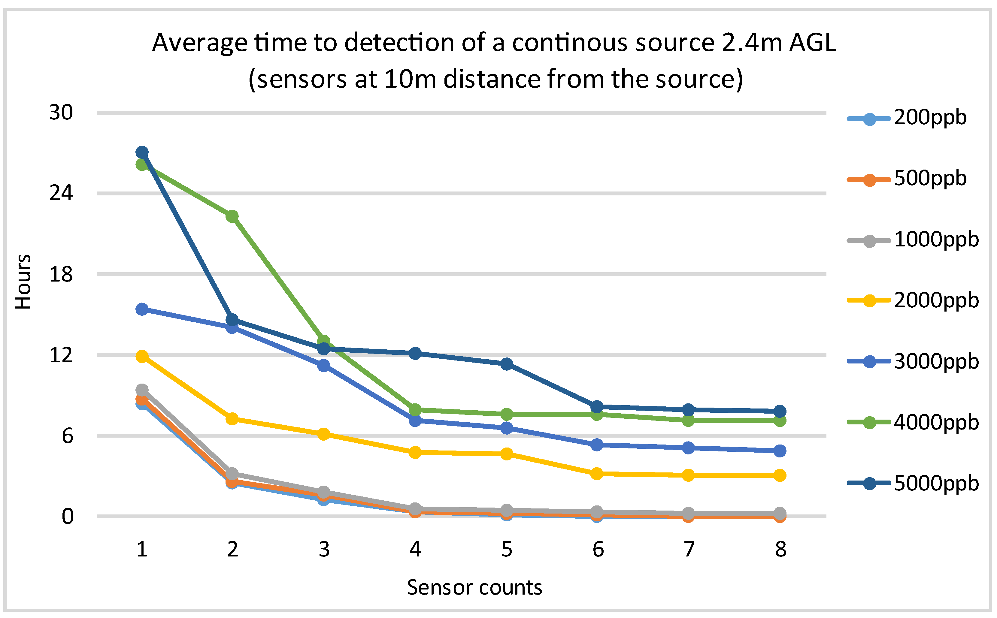
3.1. Effect of the Number of Sensors

Figure 6 shows the average detection times for a 0.4 kg/h emission source with a release point located 2.4 m agl by a group of one to eight sensors deployed 10 m from the source. Sensor placements are constrained by the eight locations, as shown in Figure 1. For each combination of sensor counts and sensor detection thresholds, optimum sensor placements are determined by maximizing the temporal coverage of detection covered by the selected locations out of the eight possible locations. A 0.4 kg/h source could be detected within 12 h, with a single sensor with a detection threshold of 2000 ppb or lower deployed 10 m from the source. The source could also be detected within 6 h, with three sensors with detection thresholds of 2000 ppb or lower. Increasing the number of sensors from one to four significantly reduces the average time to detection, whereas increasing the sensors beyond four has a limited impact on the detection times. Improving sensor detection limits or placing more sensors in the system generally reduces the average time to detection by the sensor network, but some exceptions exist, because sensor placements were optimized by maximizing temporal coverage of detection. With a similar overall temporal coverage of detection, the time to detection is affected by the temporal patterns of detection and non-detection times, represented in Figure 3.

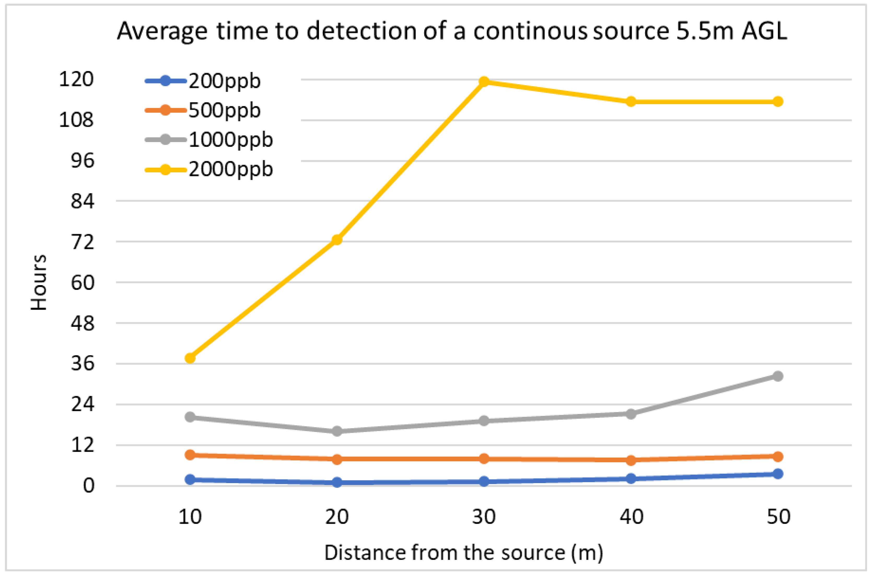
3.2. Effect of Source Release Height

The dispersion modeling simulations performed using a source height of 2.4 m agl were repeated for a source height of 5.5 m agl. Figure 7 and Figure 8 report the results of simulations for a release height of 5.5 m agl. Thresholds higher than 2 ppm led to no detection at any distances considered in this work. In general, temporal coverage was lower and time to detection higher, compared to the results for a source release height of 2.4 m. In addition, the relative performance of sensors between 10 and 20 m from the source was complex. For emission sources at the same height as the sensors (2.4 m agl), the temporal coverage and time to detection showed relatively simple monotonic behavior, as illustrated in Figure 4 and Figure 5. In contrast, for sources at 5.5 m agl, plumes may or may not reach the sensor height at distances 10 m downwind, leading to complex detection characteristics depending on the methane concentration enhancement assumed for emission detection and the meteorological conditions. This sensitivity to emission release height characteristics means that CMS performance and MDL will be sensitive to a mixture of source characteristics, including but not limited to emission rate and release height.

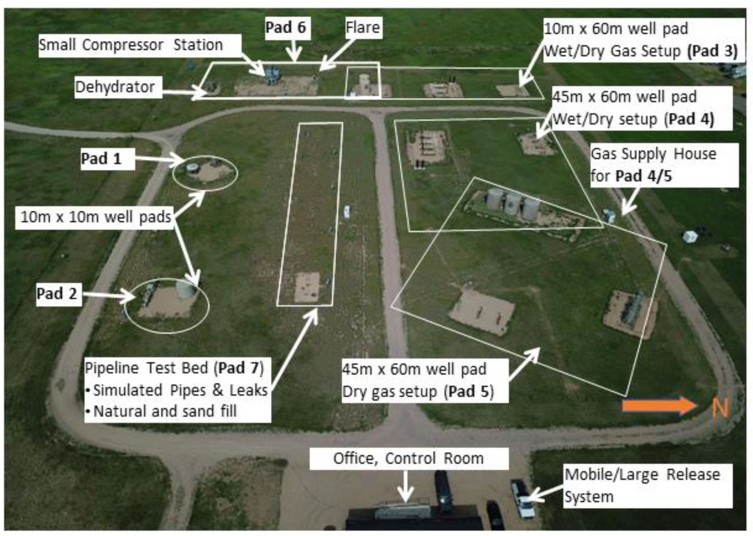
3.3. Comparison with Controlled-Release Testing

All of the analyses presented in this work assume idealized sensor performance and unobstructed plumes. Real systems will behave differently, but the overall performance predicted using dispersion modeling can be compared to the overall performance measured in controlled test facilities. Bell et al. [20] reported MDLs for eleven continuous monitoring systems deployed at the Methane Emission Technology Evaluation Center at Colorado State University (METEC) [21]. Figure 9 shows the test facility configuration, which allows for flexible sensor placement and includes a variety of emission release configurations that are representative of oil and gas facilities in the United States.

Methane emission rates ranging from 0.4 to 6400 g/h were evaluated at METEC to determine the probabilities of detection for continuous monitoring systems [20]. During testing, sensing system providers were allowed flexibility in locating their sensors and multiple sensors were frequently deployed. A typical sensor density was on the order of one per 1000 m², suggesting an average distance ~10–30 m from a source. Bell et al. [20] reported that probabilities of detection of 50–90% were achieved for multiple systems, with emission rates ranging from <0.4 to 3 kg/h. Times to detection were generally in the range of a few hours to a day. This suggests that the relatively simple source and sensor configurations used in this work are broadly representative of field conditions.

3.4. Implications

This work assessed approaches to CMS detection limits based on a simplified configuration. The framework could be widely applicable in defining detection limits for continuous monitoring systems. The dispersion modeling presented in this work demonstrates that the detection limit for continuous monitoring systems, expressed as an emission rate, will depend on meteorological conditions, the characteristics of emissions at the site, the positioning of CMS devices in relation to the emission sources, and the amount of time allowed for the CMS to detect an emission source. This means that certifying an MDL for a CMS will require a well-defined set of emission sources, with varying release heights and emission rates. Testing protocols specifying source characteristics are beginning to emerge, such as the testing scenarios employed at the METEC facility [21]. Testing protocols will also need to take into account the number and locations of sensor deployments. In testing at METEC, sensor vendors have been allowed to select sensor locations based on their understanding of the strengths and limitations of their system, and subject to logistical constraints such as the boundaries of the METEC site and the avoidance of sensor locations on site roadways.

Testing results also differ, however, depending on the meteorological conditions at the time of the test, and test results should in principle be normalized to a standard set of meteorological conditions. Those conditions might be designed to be representative of annual distributions of wind speed and wind direction in the regions in which the sensors are to be deployed, or for some other set of conditions. One mechanism for addressing meteorological variability under testing conditions would be to develop an adjustment factor based on meteorological conditions. For example, an idealized sensing system, such as the system described in this work, could be simulated for a standard set of meteorological conditions. Using the examples demonstrated in this work, an average MDL could be calculated for sources at 2.4 m agl and 5.5 m agl using the period representing annual average meteorology for the Permian Basin. The MDL could be calculated for an idealized sensor network (e.g., eight sensors deployed at 30 m from the source), where MDL could be defined as the emission rate at which idealized sensors capable of detecting a 1 ppm methane enhancement at one minute resolution would have an average time to detection of 12 h or less. Using this definition, the MDL for the meteorology used in this work would be <0.4 kg/h for sources at 2.4 m agl. For emission sources released at 5.5 m agl, the MDL would be <0.4 kg/h if the MDL is defined as a 1 ppm methane enhancement at one minute resolution and would have an average time to detection of 24 h or less. If testing was conducted under different meteorological conditions, an adjustment factor could be calculated as the ratio of MDL under test conditions and standard conditions. For example, if testing were conducted under the conditions of the first week of the two-week period, and the MDL was defined as the emission rate at which a 1 ppm methane enhancement at one minute resolution would have an average time to detection of 12 h or less for a network of eight sensors deployed 30 m from a source at 2.4 m agl, then the MDL would be 0.13 kg/h. If testing was conducted under the conditions of the second week of the two-week period analyzed in this work, the MDL would be 0.10 kg/h. If testing was carried out during both weeks, the MDL would be 0.11 kg/h. An approach such as this would allow for the consistent field testing of CMS technologies while recognizing the importance of meteorological conditions in evaluating performance characteristics.

References

1. Saunois, M.; Stavert, A.R.; Poulter, B.; Bousquet, P.; Canadell, J.G.; Jackson, R.B.; Raymond, P.A.; Dlugokencky, E.J.; Houweling, S.; Patra, P.K.; et al. The global methane budget 2000–2017. Earth Syst. Sci. Data Discuss. 2020, 12, 1561–1623. [Google Scholar] [CrossRef]
2. National Academies of Sciences, Engineering, and Medicine. Improving Characterization of Anthropogenic Methane Emissions in the United States; The National Academies Press: Washington, DC, USA, 2018. [Google Scholar]
3. Zavala-Araiza, D.; Lyon, D.R.; Alvarez, R.A.; Davis, K.J.; Harriss, R.; Herndon, S.C.; Karion, A.; Kort, E.A.; Lamb, B.K.; Lan, X.; et al. Reconciling divergent estimates of oil and gas methane emissions. Proc. Natl. Acad. Sci. USA 2015, 112, 15597–15602. [Google Scholar] [CrossRef] [PubMed]
4. Zavala-Araiza, D.; Alvarez, R.A.; Lyon, D.R.; Allen, D.T.; Marchese, A.J.; Zimmerle, D.J.; Hamburg, S.P. Super-emitters in natural gas infrastructure are caused by abnormal process conditions. Nat. Commun. 2017, 8, 14012. [Google Scholar] [CrossRef] [PubMed]
5. United Nations Environment Program. Methane Alert and Response System. 2023. Available online: https://www.unep.org/explore-topics/energy/what-we-do/methane/imeo-action/methane-alert-and-response-system-mars (accessed on 26 December 2023).
6. United States Greenhouse Gas Center. 2023. Available online: https://earth.gov/ghgcenter (accessed on 26 December 2023).
7. Varon, D.J.; Jacob, D.J.; McKeever, J.; Jervis, D.; Durak, B.O.; Xia, Y.; Huang, Y. Quantifying methane point sources from fine-scale satellite observations of atmospheric methane plumes. Atmos. Meas. Tech. 2018, 11, 5673–5686. [Google Scholar] [CrossRef]
8. Jacob, D.J.; Varon, D.J.; Cusworth, D.H.; Dennison, P.E.; Frankenberg, C.; Gautam, R.; Guanter, L.; Kelley, J.; McKeever, J.; Ott, L.E.; et al. Quantifying methane emissions from the global scale down to point sources using satellite observations of atmospheric methane. Atmos. Chem. Phys. 2022, 22, 9617–9646. [Google Scholar] [CrossRef]
9. Chen, Q.; Modi, M.; McGaughey, G.; Kimura, Y.; McDonald-Buller, E.; Allen, D.T. Simulated methane emission detection capabilities of continuous monitoring networks in an oil and gas production region. Atmosphere 2022, 13, 510. [Google Scholar] [CrossRef]
10. Wang, J.L.; Daniels, W.S.; Hammerling, D.M.; Harrison, M.; Burmaster, K.; George, F.C.; Ravikumar, A.P. Multiscale methane measurements at oil and gas facilities reveal necessary frameworks for improved emissions accounting. Environ. Sci. Technol. 2022, 56, 14743–14752. [Google Scholar] [CrossRef] [PubMed]
11. United Nations. Oil and Gas Methane Partnership (OGMP) 2.0 Framework; Climate & Clean Air Coalition; 2020; Available online: https://www.ccacoalition.org/resources/oil-and-gas-methane-partnership-ogmp-20-framework (accessed on 26 December 2023).
12. United Nations. List of OGMP 2.0 Member Companies (as of 11.03.2024). 2024. Available online: https://ogmpartnership.com/wp-content/uploads/2024/03/List_of_OGMP2.0_Member_Companies_11.03.pdf (accessed on 10 March 2024).
13. United States Environmental Protection Agency. Greenhouse Gas Reporting Rule: Revisions and Confidentiality Determinations for Petroleum and Natural Gas Systems (GHG Reporting Rule), proposal published in the Federal Register, 88, 50282, 1 August 2023. Available online: https://www.federalregister.gov/documents/2023/08/01/2023-14338/greenhouse-gas-reporting-rule-revisions-and-confidentiality-determinations-for-petroleum-and-natural (accessed on 26 December 2023).
14. United States Environmental Protection Agency. Standards of Performance for New, Reconstructed, and Modified Sources and Emissions Guidelines for Existing Sources: Oil and Natural Gas Sector Climate Review. 2023. Available online: https://www.epa.gov/system/files/documents/2023-12/eo12866_oil-and-gas-nsps-eg-climate-review-2060-av16-final-rule-20231130.pdf (accessed on 26 December 2023).
15. Chen, Q.; Schissel, C.; Kimura, Y.; McGaughey, G.; McDonald-Buller, E.; Allen, D.T. Assessing detection efficiencies for continuous methane emission monitoring systems at oil and gas production sites. Environ. Sci. Technol. 2023, 57, 1788–1796. [Google Scholar] [CrossRef] [PubMed]
16. Texas Railroad Commission. Permian Basin Information. 2023. Available online: https://www.rrc.texas.gov/oil-and-gas/major-oil-and-gas-formations/permian-basin/ (accessed on 16 August 2023).
17. University of Texas, Project Astra Web Site. 2023. Available online: https://dept.ceer.utexas.edu/ceer/astra/ (accessed on 26 December 2023).
18. Exponent. Official CALPUFF Modeling System. 2020. Available online: http://www.src.com/ (accessed on 26 December 2023).
19. Torres, V.M.; Sullivan, D.W.; He’Bert, E.; Spinhirne, J.; Modi, M.; Allen, D.T. Field inter-comparison of low-cost sensors for monitoring methane emissions from oil and gas production operations. Atmos. Meas. Tech. Discuss. 2022, 2022, 1–22. [Google Scholar]
20. Bell, C.; Ilonze, C.; Duggan, A.; Zimmerle, D. Performance of Continuous Emission Monitoring Solutions under a Single-Blind Controlled Testing Protocol. Environ. Sci. Technol. 2023, 57, 5794–5805. [Google Scholar] [CrossRef] [PubMed]
21. Methane Emissions Technology Evaluation Center (METEC). Colorado State University. 2023. Available online: https://energy.colostate.edu/metec/ (accessed on 26 December 2023).
Figure 1. Source and sensor locations are deployed radially in concentric rings every 45 degrees, at 10 m, 20 m, 30 m, 40 m, and 50 m from a source emitting at 0.4 kg/h.
Atmosphere 15 00383 g001
Figure 2. Wind rose for the two-week episode used in dispersion modeling.
Atmosphere 15 00383 g002
Figure 3. Time series of periods of detection and non-detection for a group of 8 sensors located 20 m from a source with a release rate of 0.4 kg/s and a release height of 2.4 m agl.
Atmosphere 15 00383 g003
Figure 4. Fraction of time that a 0.4 kg/h emission source with a release point located 2.4 m agl would be observed by at least one of eight sensors deployed every 45 degrees at various distances from the source.
Atmosphere 15 00383 g004
Figure 5. Detection times for a 0.4 kg/h emission source with a release point located 2.4 m agl by a group of 8 sensors deployed every 45 degrees at various distances from the source.
Atmosphere 15 00383 g005
Figure 6. Detection times for a 0.4 kg/h emission source with a release point located 2.4 m agl by a group of 1 to 8 sensors deployed at a 10 m distance from the source.
Atmosphere 15 00383 g006
Figure 7. Fraction of time that a 0.4 kg/h emission source with a release point located 5.5 m agl would be observed by at least one of eight sensors deployed every 45 degrees at various distances from the source.
Atmosphere 15 00383 g007
Figure 8. Detection times for a 0.4 kg/h emission source with a release point located 5.5 m agl by a group of 8 sensors deployed every 45 degrees at various distances from the source.
Atmosphere 15 00383 g008
Figure 9. The Methane Emissions Technology Evaluation Center (METEC), designed to perform controlled-release testing in a configuration that simulates upstream oil and gas facilities [20,21].
Atmosphere 15 00383 g009
Disclaimer/Publisher’s Note: The statements, opinions and data contained in all publications are solely those of the individual author(s) and contributor(s) and not of MDPI and/or the editor(s). MDPI and/or the editor(s) disclaim responsibility for any injury to people or property resulting from any ideas, methods, instructions or products referred to in the content.