Evaluating the Effects of Raindrop Motion on the Accuracy of the Precipitation Inversion Algorithm by X-SAR

Abstract

Precipitation has a profound impact on both human life and the natural environment. X-band synthetic aperture radar (X-SAR) utilizes high-resolution microwave remote-sensing technology, providing opportunities for global precipitation measurements. The current precipitation inversion algorithms from X-SAR measurements assume that precipitation particles remain relatively stationary with the ground. However, the motion of raindrops could potentially reduce the accuracy of these algorithms. In this study, we first established a functional relationship between raindrop motion and SAR echoes based on the standard deviation of the raindrop Doppler velocity spectrum. Secondly, an exploratory algorithm was proposed to retrieve rainfall distribution under the raindrop motion error model (RMM) and quantitatively calculate the precipitation inversion error caused by raindrop motion. In comparison to conditions where the atmosphere is stationary, when the standard deviation of the Doppler velocity spectrum of raindrops is 1.1 m/s, the relative error of the retrieved surface rain rate increases from 2.1% to 35.8%. Numerical simulations show that SAR echoes are sensitive to changes in the standard deviation of the Doppler velocity spectrum, and the impact of raindrop motion on the accuracy of X-SAR precipitation measurements cannot be neglected.

1. Introduction

In the atmospheric, hydrological, oceanic, and environmental sciences, the study of rainfall is a very important component. Precipitation consists of a collection of liquid or solid water particles, known as hydrometeors, that begin within a cloud. The measurement of global precipitation is a major goal in environmental climate change research [1]. International satellite missions, such as the tropical rainfall measuring mission (TRMM) [2] and the global precipitation mission (GPM) [3], enhance the advancements in satellite-based global precipitation measurements.

The X-band spaceborne synthetic aperture radar (X-SAR) satellite TerraSAR-X was successfully launched in 2007. It can acquire high-resolution images of any desired area, regardless of weather conditions, with a resolution of up to 1 m [4]. With the rapid development of numerous satellite platforms equipped with high spatial resolution SAR technology, the application of SAR high-resolution ground data in various fields, such as water body detection, optical image enhancement, target detection, and terrain recognition, is becoming increasingly widespread [5,6,7,8]. The traditional methods of estimating rainfall using rain gauges and land-based radars do not cover the entire world, particularly ocean areas [9]. Satellite remote-sensing technology, however, can provide more comprehensive precipitation distribution information with its broad coverage and high-frequency measurements. The numerous inherent advantages of SAR provide the possibility for more convenient, nearly global, continuous, and high-precision precipitation inversion [10,11,12]. Consequently, exploring how to utilize SAR for global precipitation monitoring holds significant implications for complementing the theory of precipitation measurements and meeting practical needs.

Research shows that the X band (10 GHz) near the Ku band (14 GHz), used by precipitation radar (PR), is more sensitive to rainfall effects than the L and C bands [13,14]. Moore et al. (1997) observed SAR images and found that rain clouds were evident in both C-band and X-band images. For the first time, they used echo signals and image shadows to determine precipitation, showcasing the potential of spaceborne X-SAR for precipitation inversion [14]. Pichugin et al. (1991) assumed a uniform distribution of precipitation in the vertical direction under a single-layer rainfall model [15]. By introducing a particular function, they cleverly converted the non-linear expression for rainfall attenuation into a linear Volterra integral equation (VIE) of the second kind. This transformation made the task of rainfall retrieval straightforward. The VIE algorithm achieves high inversion accuracy but cannot be directly applied to models containing two or more meteorological particles. When this method is applied to vertically non-uniform models, the computational complexity of the analytical solution significantly increases. Marzano et al. (2008) proposed the model-oriented statistical (MOS) inversion algorithm [16]. This method can retrieve precipitation distribution for a double-layer rainfall model with a completely separated snowfall layer and rainfall layer. However, it requires a large number of empirical parameters. MOS has high accuracy in rainstorms but performs poorly in light to moderate rain. Weinman et al. (2009) used precipitation data from Bangladesh and the Amazon region for inversion. The relative errors of the MOS and VIE algorithms are both within 20% [17], which makes them applicable for rainfall inversion in real-life scenarios. Zheng et al. (2020) proposed a method for detecting rainfall based on the correlation characteristics of the sea clutter and the difference in the correlation coefficients between sea wave images with and without rain. This method can detect rainfall from X-SAR images with uneven precipitation distribution [18]. Zhao et al. (2021) used textural information to detect and segment rainfall on sea surface SAR images [19].

However, there are still several issues with spaceborne X-SAR precipitation measurement technology, one of which is the potential error caused by neglecting the movement of raindrops. Numerous studies show links between wind fields, raindrop motion, and SAR images. Draper and others conducted experiments that provided evidence of rainfall causing a significant attenuation in the C-band SAR backscattering cross section of the sea surface wind [20]. Satake et al. analyzed the polarimetric data of rainfall obtained from an airborne X-SAR and explored the relationship between raindrop motion and SAR images [21]. Yu found that heavy rain could reduce the accuracy of wind speed measurement by SAR up to 30%, especially under typhoon conditions, becoming more complex with increasing rainfall intensity [22]. Studies focusing on rain effects on wind field retrieval have developed methods to recognize heavy rain-affected areas and reconstruct SAR-retrieved wind speed in those areas [23,24]. However, many interesting rain-related phenomena revealed by SAR images are still not fully understood due to poor theoretical modeling of the rain–wind–wave interactions [25].

Our knowledge of the effects of wind-induced raindrop motion on SAR data limits the current precipitation retrieval methods. When SAR detects distributed targets such as precipitation, it assumes that the precipitation particles remain relatively stationary with the ground. In the actual rainfall environment, raindrop motion can impact the inversion model and introduce errors in the inversion of precipitation intensity. However, there is currently no publicly available quantitative analysis of the error caused by raindrop motion in SAR precipitation retrieval in the existing literature. The research on SAR precipitation measurements needs to include the content of raindrop motion error. To address the above problems, this paper establishes a raindrop motion error model and studies the impact of the standard deviation of the Doppler velocity spectrum of precipitation particles on SAR backscattering echoes. Subsequently, we propose an algorithm based on the raindrop motion error model (RMM). Combined with the MOS inversion method, the RMM algorithm can quantify the wind-induced raindrop motion’s impact on precipitation retrieval accuracy.

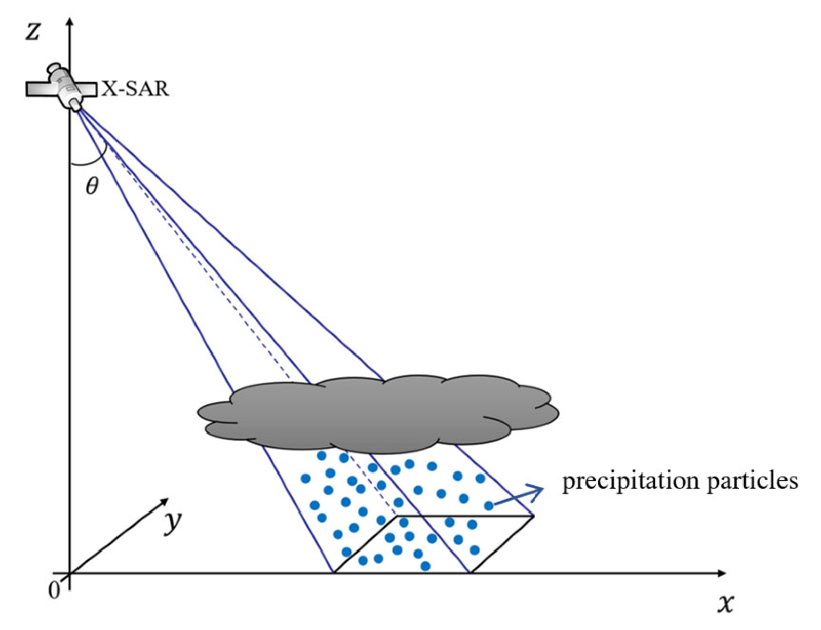
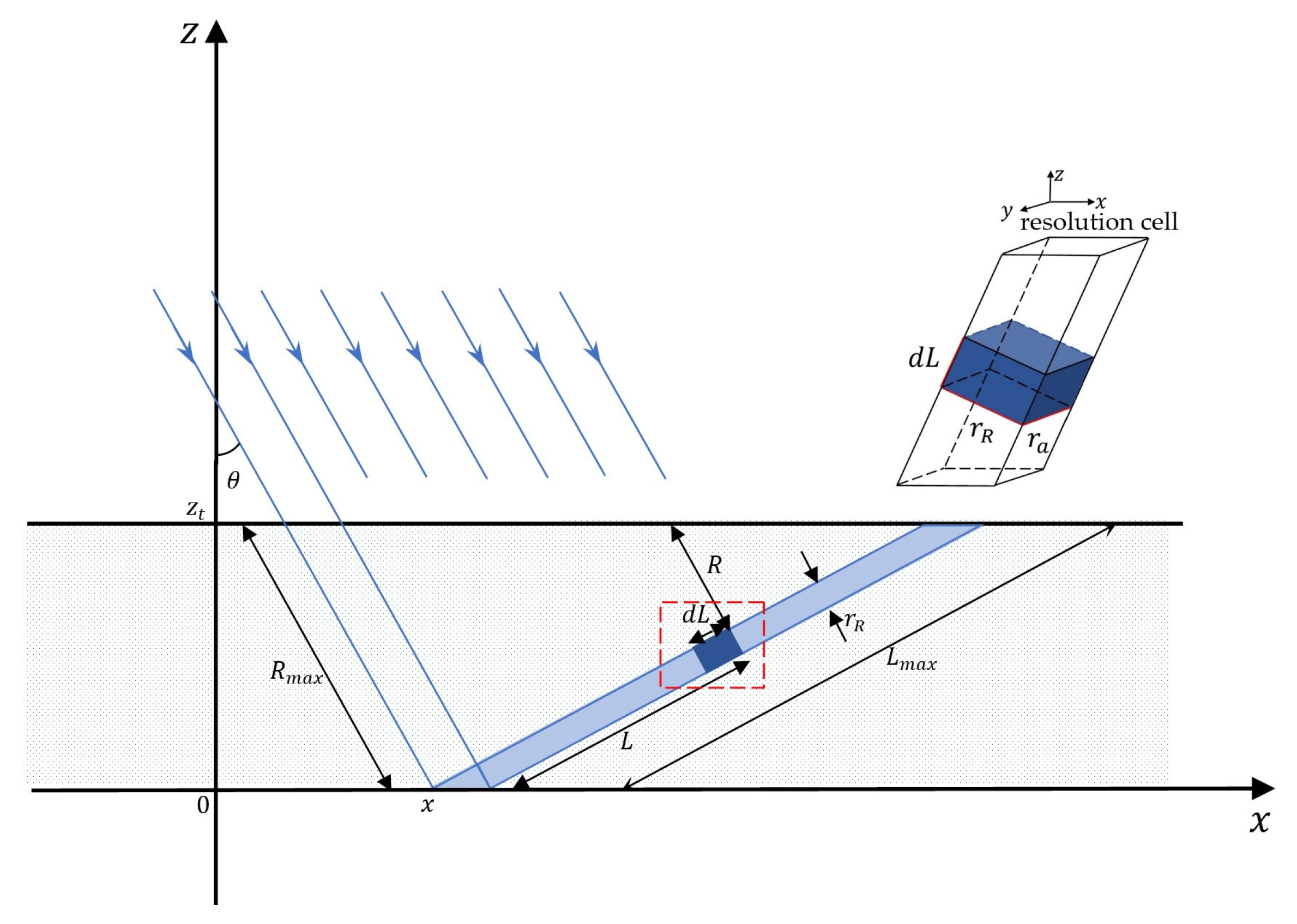
2. SAR Rain Measurement Principles

The radar cross section (RCS) in ${\mathrm{m}}^2$ is used to describe the backscattering characteristics of a target [26]:

$$\sigma (r,\theta ,\phi )=4\pi r^2\frac{S_s(r,\theta ,\phi )}{S_i(r,{\theta }_i,{\phi }_i)}$$

(1)

where the dimension of $\sigma$ is the area, $\theta$ is the slant off-nadir angle, and $\phi$ is the azimuth angle, respectively. $S_s$ is the backscattering power density, and $S_i$ is the incident power density in the $(\theta ,\phi )$ direction.

The three-dimensional side view of precipitation detection by SAR is shown in Figure 1. The x-axis is the cross-track direction, the y-axis is the along-track direction, and the z-axis is the altitude direction.

Figure 1. SAR side view three-dimensional structure diagram.

Assuming that the backscattering echoes of precipitation particles within a radar beam are incoherent, the energy of the total backscattering echoes is equal to the sum of the echo energy of each particle. When SAR detects precipitation in strip scan mode, the power of the backscattering echoes is as follows [26]:

$$P_r=\frac{P_t{G}^2{\lambda }^2}{{\left(4\pi \right)}^2{r}^4}\sum _{i=1}^N{\sigma }_i$$

(2)

where $P_r$ is the radar received power, $P_t$ is the radar transmitted power, $G$ is the radar antenna gain, $\lambda$ is the operating wavelength, $r$ is the distance between the measured target and the radar, $N$ is the total number of precipitation particles within the effective illuminated volume of the radar beam that simultaneously produce scattering echo energy and return to the radar antenna, and ${\sigma }_i$ is the backscattering cross section of an individual precipitation particle.

The radar volume reflectivity of precipitation is defined as the sum of the backscattering cross section of all precipitation particles per unit volume, denoted as $\eta$ [27]:

$$\eta =\sum {\sigma }_i$$

(3)

The volume resolution cell represents the minimum separable precipitation unit that SAR can distinguish during motion. It can be considered as the differential element of the effective illuminated volume. The volume of the cell is related to the three-dimensional resolutions of SAR [28]:

$$V_r=r_R{r}_c{r}_a$$

(4)

where $r_R$ is the slant-range resolution, $r_a$ is the azimuth resolution, and $r_c$ is the resolution corresponding to the beam width in the pitch plane.

In practical applications, SAR precipitation measurements need to consider the impact of precipitation particles on the attenuation of radar echoes. L is the one-way attenuation factor. Therefore, the backscattering echoes power for detecting precipitation with SAR within the volume resolution cell can be expressed as follows:

$$P_r=\frac{P_t{G}^2{\lambda }^2{V}_r\eta }{{\left(4\pi \right)}^2{r}^4}{L}^2$$

(5)

Therefore, the sum of the radar backscattering cross sections of all precipitation particles within the volume resolution cell is as follows:

$$\sigma =V_r\eta L^2$$

(6)

The observation range of spaceborne SAR is typically extensive with significant variations in $\sigma$. Instead, we generally use the dimensionless normalized radar cross section (NRCS), denoted as ${\sigma }_{SAR}$, which is obtained by comparing it with the area. The transformation relationship between $\sigma$ and ${\sigma }_{SAR}$ will be discussed in detail in Section 4.1.

The absorption and scattering of radar waves by precipitation particles between the radar and the target cause signal attenuation. In radar meteorology, the precipitation particles’ attenuation and scattering effects on electromagnetic waves are typically described by the power law relationship [29,30]. The relationship between the rainfall attenuation coefficient $k(x,z)$ in $\mathrm{k}{\mathrm{m}}^{-1}$, radar reflectivity $\eta (x,z)$ in $\mathrm{k}{\mathrm{m}}^{-1}$, and precipitation $R(x,z)$ in mm/h is summarized as follows:

$$\eta (x,z)=\frac{{\pi }^5}{{\lambda }^4}{\left|K_0\right|}^{2}i{R(x,z)}^j$$

(7)

$$k(x,z)\approx a{R(x,z)}^b$$

(8)

where ${\left|K_0\right|}^2$ is a function of the refractive index of water when neglecting the influence of temperature; the value of ${\left|K_0\right|}^2$ is approximately 0.93 for rain and 0.19 for snow [13]. In this paper, the relevant empirical parameters $a,b,i,$ and $j$ adopt the typical values statistically calculated by Ulaby et al. For rain, a is 2.6 × 10⁻³, b is 1.11, i is 300, and j is 1.35; for snow, a is 5.6 × 10⁻³, b is 1.60, i is 182, and j is 1.60 [31].

From Equations (5), (7), and (8), the precipitation distribution information can be retrieved using SAR echo data, which is the fundamental principle of SAR precipitation measurements.

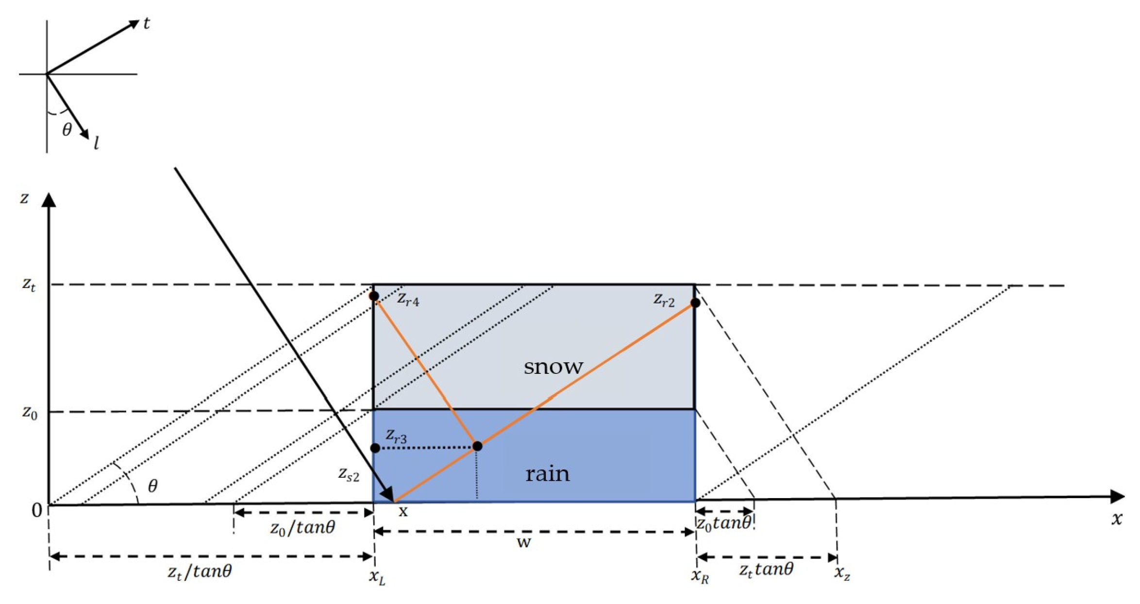
3. Raindrop Motion Error Model

When SAR detects distributed targets like precipitation, it assumes that the precipitation particles remain relatively stationary with the ground. In the actual precipitation environment, the echo signal received by the radar is influenced by various factors, such as raindrop motion, atmospheric turbulence, and the effect of surface horizontal winds. The signal is the comprehensive result of the backscattering of all scattering particles within the effective illuminated volume. Such a comprehensive result leads to the standard deviation of the Doppler velocity spectrum, indicating that the echo signal contains multiple frequency components. Raindrop motion affects the azimuthal resolution of SAR precipitation measurement that, in turn, affects the precipitation volume resolution cell, echo intensity, and other factors [23].

Spaceborne SAR is a two-dimensional, high-resolution microwave imaging radar. It achieves high resolution in range by transmitting large bandwidth signals and achieves high resolution in azimuth by synthetic aperture technology [32]. Under the impact of raindrop motion, the equivalent azimuthal resolution is as follows [33]:

$$r_a=\frac{2{\sigma }_v}{u}r$$

(9)

where $u$ is the platform speed, $r$ is the distance between SAR and the measured target, and ${\sigma }_v$ is the standard deviation of the Doppler speed spectrum of raindrops. The Doppler speed spectrum width characterizes the extent to which various sizes of Doppler speeds within the effective illuminated volume deviate from their average value, which is caused by the different radial velocities of the scattering particles. When SAR measures distributed targets such as raindrops, ${\sigma }_v$ is variable under different meteorological conditions [34]. It is approximately 0.6 m/s for snowfall in a stationary atmosphere and 10 m/s for rainfall in strong wind shear. In practical calculations, ${\sigma }_v$ takes 1 m/s as the typical value for rainfall in a stationary atmosphere [26].

Based on the analysis above, a positive linear relationship exists between the standard deviation of the raindrop Doppler velocity spectrum and the azimuthal resolution of SAR precipitation measurements. On this basis, we establish the raindrop motion error model, as shown in Figure 2. First, consider calculating the SAR backscattering cross section under the ideal rain cloud with a uniform distribution of precipitation in both the horizontal and vertical directions. We analyze the propagation of electromagnetic waves and backscattering situations to derive a calculation method for the SAR backscattering cross section in the raindrop motion model in the following.

Figure 2. Raindrop motion error model. (Below) The geometry for calculating attenuation of the returns from different parts of the rain resolution cell; (Upper right) The three-dimensional structure of the rain resolution cell.

In Figure 2, $\theta$ is the incident angle, $z_t$ is the cloud top height, and $R$ is the distance in the rain for attenuation for a differential element on the x-z plane with a maximum length of $R_{max}$ in km. $L$ is the distance from the surface to a differential volume for rain scatter on the x-z plane with a maximum length of $L_{max}$ in km.

The beam below the cloud top is divided into resolution cells corresponding to the slant range resolution $r_R$. The light blue area in the center of Figure 2 shows one of the rain resolution cells. The thickness of the cell is the slant range resolution $r_R$. The width of the cell is the azimuth resolution $r_a$. It is noteworthy that, on the incident plane, the length of the rain resolution cell is $L_{max}$, perpendicular to the direction from the radar to the rain, while the length of the illuminated volume defined by the three-dimensional resolutions corresponds to the differential amount dl. From Figure 2, we can derive the following relationship:

$$\frac{R}{R_{max}}=\frac{(L_{max}-L)}{L_{max}}$$

(10)

$$R_{max}=\frac{z_t}{cos\theta }$$

(11)

$$L_{max}=\frac{z_t}{sin\theta }$$

(12)

Then, we can obtain the following:

$$R=(1-\frac{Lsin\theta }{z_t})\frac{z_t}{cos\theta }$$

(13)

The volume of the rain resolution cell from the bottom and the ground area coupled to the rain cell can be calculated as follows [14]:

$$V=r_a{r}_R{L}_{max}$$

(14)

$$A=\frac{r_a{r}_R}{sin\theta }$$

(15)

The total radar backscattering cross section is the sum of the two components:

$$\sigma ={\sigma }_{srf}+{\sigma }_{vol}$$

(16)

The ideal rain cloud assumes a uniform distribution of precipitation in both the horizontal and vertical directions. From Equations (7) and (8), we can infer that a certain amount of precipitation corresponds to fixed values of the attenuation coefficient $k$ and the radar reflectivity $\eta$. Without taking into account the attenuation of electromagnetic waves along the propagation path, the surface backscattering cross section ${\sigma }_{srf}$ and the precipitation backscattering cross section ${\sigma }_{vol}$ can be expressed as follows:

$${\sigma }_{srf}={\sigma }^0\frac{r_a{r}_R}{sin\theta }$$

(17)

$${\sigma }_{vol}=r_a{r}_R{L}_{max}\eta$$

(18)

where ${\sigma }^0$ is the average backscattering cross section for vertically polarized radiation incident on land at 30°, which is approximately −7 dB [35].

Now consider a more realistic situation where different parts of each rain resolution cell experience different attenuation paths for backscattering. The closer to the top of the rain cloud, the smaller the attenuation. Near the top of the rain cloud, little attenuation occurs. The attenuation factors $K_{srf}$ and $K_{vol}$ are used to characterize the attenuation effect on the ground surface and precipitation backscattering echoes in the actual precipitation environment. Equations (17) and (18) can be rewritten as follows:

$${\sigma }_{srf}={\sigma }_{srf}{K}_{srf}={\sigma }_{srf}{e}^{-2k{R}_{max}}={\sigma }_{srf}{e}^{\frac{-2k{z}_t}{cos\theta }}$$

(19)

$${\sigma }_{vol}={\sigma }_{vol}{K}_{vol}=\eta r_a{r}_R{\int }_0^{L_{max}}{e}^{-2k\frac{z_t}{cos\theta }(1-\frac{Lsin\theta }{z_t})}dL$$

(20)

Assume that the effective volume of the rain cell in the actual rainfall environment is $V_{eff}$. Calculating the integral in Equation (20) and substituting in the definition of $V_{eff}$, we obtain the following:

$$V_{eff}=r_a{r}_R\frac{1-e^{-2k{z}_t/cos\theta }}{2ktan\theta }=V\frac{1-e^{-2k{z}_t/cos\theta }}{2k{z}_t/cos\theta }$$

(21)

In summary, the surface backscattering cross section and the volume backscattering cross section in the actual precipitation environment, considering the raindrop motion, can be expressed as follows:

$${\sigma }_{srf}=\frac{{\sigma }^0{r}_a{r}_R}{sin\theta }{e}^{\frac{-2k{z}_t}{cos\theta }}$$

(22)

$${\sigma }_{vol}=\frac{r_a{r}_R\eta }{2ktan\theta }(1-e^{\frac{-2k{z}_t}{cos\theta }})$$

(23)

where $r_a$ is the equivalent azimuthal resolution, which varies with the standard deviation of the Doppler velocity spectrum of raindrops. ${\sigma }_v$ generally ranges from 0.6 to 8.0 m/s.

Under the raindrop motion model established in this paper, we derive formulas for calculating the effective surface and precipitation backscattering under different standard deviations of the Doppler velocity spectrum. This allows for further analysis of the SAR radar scattering cross section changes caused by raindrop motion.

4. RMM Algorithm

The RMM algorithm merges the proposed raindrop motion error model with the MOS inversion algorithm, enabling a quantitative evaluation of the impact of raindrop motion on the accuracy of MOS. The overall RMM algorithm is schematically shown in Figure 3, and each step is illustrated in the following.

Figure 3. The process of RMM.

4.1. RCS and NRCS

The RMM algorithm uses simulated SAR echo data with raindrop motion errors as equivalent SAR echo data. Under the raindrop motion error model, we can calculate the RCS with varying levels of raindrop motion error by controlling the standard deviation of the raindrop Doppler velocity spectrum. Since the MOS algorithm uses NRCS data as the input, we first need to normalize the RCS to NRCS to quantitatively analyze the raindrop motion’s impact on the MOS accuracy.

The X-SAR precipitation measurement model used to calculate the NRCS is shown in Figure 4. This model neglects the earth’s curvature, does not consider beam width, and simplifies spherical waves into plane waves for analysis.

Figure 4. Schematic view of the model used to compute the NRCS from a double-layer rain cloud.

The NRCS is derived from the surface backscattering cross section from the ground and the volume backscattering cross section from precipitation [10], as follows:

$${\sigma }_{SAR}={\sigma }^0{e}^{-2{\int }_{z_{s1}}^{z_{s2}}k\left(z\right)dz/cos\theta }+{\int }_{z_{r1}}^{z_{r2}}\eta \left(z\right)e^{-2{\int }_{z_{r3}}^{z_{r4}}k\left(z^{\prime }\right)d{z}^{\prime }/cos\theta }dz$$

(24)

where $z_{s2}$ and $z_{s1}$ and $z_{r4}$ and $z_{r3}$ are, respectively, the upper and lower attenuation limits of backscattering echoes from the surface and the volume resolution cell. $z_{r2}$ and $z_{r1}$ are the upper and lower limits of the resolution cell in the rainfall area. $z_0$ is the top height of the rain layer, and $z_t$ is the top height of the snow layer. The rain cloud width $w$ extends from the left corner $x_L$ to the right corner $x_R$.

Based on the analysis in Section 3, we can similarly derive the radar backscattering cross section for the double-layer rain cloud shown in Figure 4:

$$\sigma ={\sigma }_{srf}+{\sigma }_{vol}=\frac{r_a{r}_R}{sin\theta }{\sigma }^0{e}^{-2{\int }_{z_{s1}}^{z_{s2}}k\left(z\right)dz/cos\theta }+r_a{r}_R{\int }_{z_{r1}}^{z_{r2}}\eta \left(z\right)e^{-2{\int }_{z_{r3}}^{z_{r4}}k\left(z^{\prime }\right)d{z}^{\prime }/cos\theta }dz$$

(25)

Thus, we can also obtain the conversion relationship between NRCS and RCS as follows:

$${\sigma }_{SAR}=\frac{sin\theta }{r_a{r}_R}{\sigma }_{srf}+\frac{{\sigma }_{vol}}{{r_{a}r}_R}$$

(26)

where ${\sigma }_{SAR}$ denotes the NRCS data; the surface backscattering cross section ${\sigma }_{srf}$ and the volume backscattering cross section ${\sigma }_{vol}$ are the two components of the RCS.

Next, we use a simple example to illustrate how errors are introduced into the MOS in the RMM algorithm. Assuming ${\sigma }_{v1}$ = 1 m/s and ${\sigma }_{v2}$ = 2 m/s, the relationship can be obtained from Equation (9):

$$r_{a2}=2r_{a1}$$

(27)

The original MOS algorithm does not consider raindrop motion and only applies to a windless situation with ${\sigma }_v$ = 1 m/s. When the actual rainfall environment is windy with ${\sigma }_v$ = 2 m/s, the NRCS, used as the input data to the algorithm, contains a certain degree of motion error. We use ${\sigma }_{mSAR}$ to represent the NRCS data with the raindrop motion error as follows:

$${\sigma }_{mSAR}=\frac{sin\theta }{r_{a1}{r}_R}{\sigma }_{srf2}+\frac{{\sigma }_{vol2}}{{r_{a1}r}_R}=2{\sigma }_{SAR}$$

(28)

A conclusion can be drawn about the conversion relationship. For the double-layer rain cloud model in Figure 4, the sizes of the two sets of NRCS data satisfy a proportional relationship when the standard deviation of the raindrop Doppler velocity spectrum ${\sigma }_v$ is taken as 1 m/s and 2 m/s, respectively. The difference between the two is 3 dB when converted into decibels.

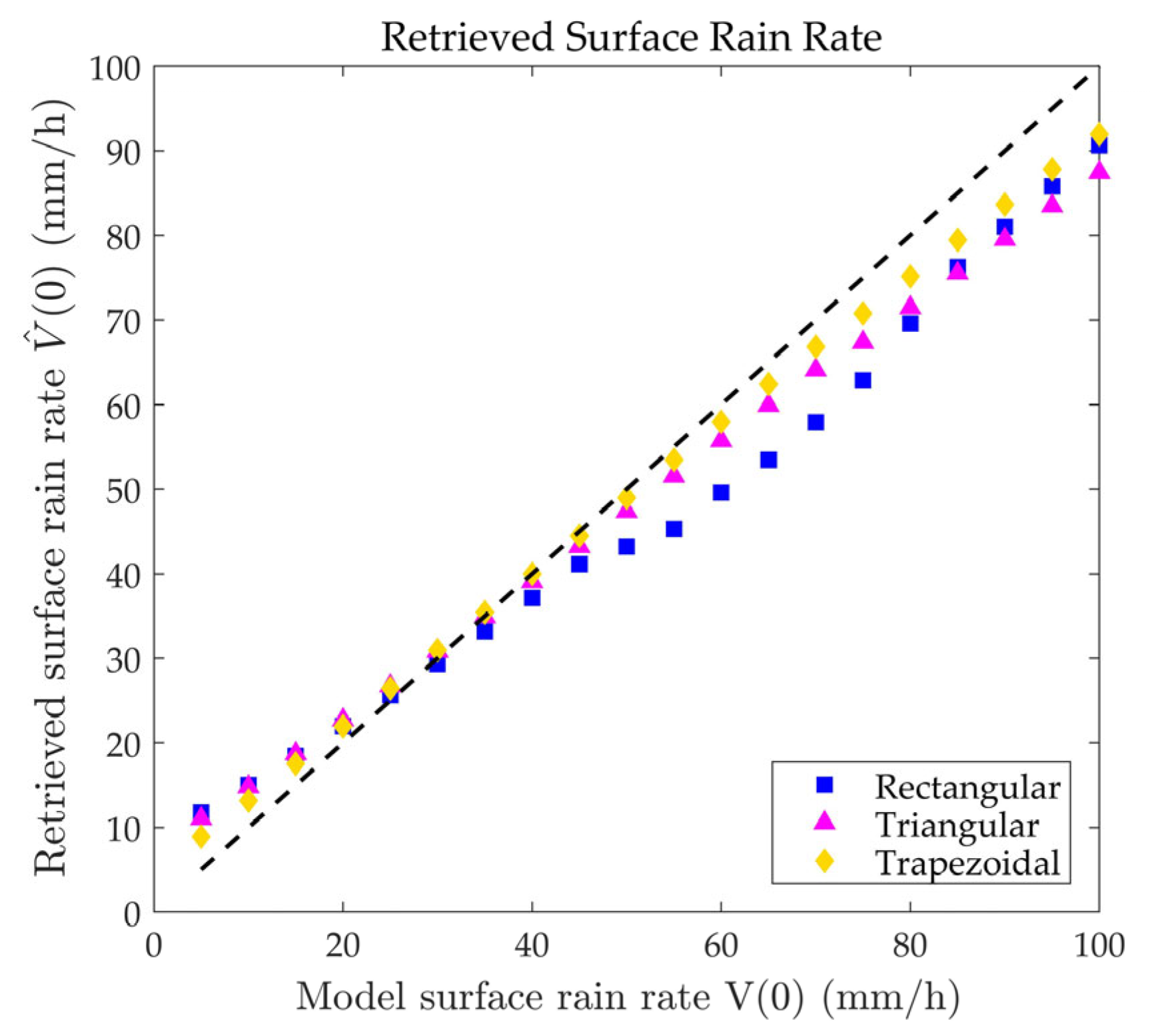
4.2. Retrieval of Precipitation Distribution

The RMM mainly uses the MOS inversion method to obtain precipitation distribution. The spatial distribution of precipitation can be categorized into different types [36]. To simplify the problem, it assumes that the two-dimensional precipitation distribution $R(x,z)$ can be divided into horizontal and vertical distributions. The two distributions are considered uncorrelated and can be retrieved separately:

$$R\left(x,z\right)=H\left(x\right)V\left(z\right)$$

(29)

The horizontal weighting factor $H\left(x\right)$ varies linearly and symmetrically with the distance from the edges over a thickness d:

$$H\left(x\right)=\left\{\begin{array}{cc}\hfill 0,& 0\le x<z_t/\tan \theta \hfill \\ \hfill x/d-z_t/(\mathrm{dtan}\theta ),& z_t/\tan \theta \le x<d+z_t/\tan \theta \hfill \\ \hfill 1,& d+z_t/\tan \theta \le x<w-d+z_t/\tan \theta \hfill \\ \hfill (w-x)/d+z_t/(\mathrm{dtan}\theta ),& w-d+z_t/\tan \theta \le x<w+z_t/\tan \theta \hfill \\ \hfill 0,& x\ge w+z_t/\tan \theta \hfill \end{array}\right.$$

(30)

There are 18 existing types of $H\left(x\right)$ [37]. The three most commonly used are rectangular (d = 0), trapezoidal (0 < d < w/2), and triangular (d = w/2) horizontal distributions. In this paper, the parameters with superscripts represent the retrieved values, while the parameters without superscripts represent the given values. By applying the concept of maximum likelihood classification to the ${\sigma }_{SAR}$ data analysis, we can obtain $\widehat{H}(x)$ [38]. The MOS inversion method performs statistical calculations on simulated NRCS data, yielding the mean vector $m_{cSAR}$ and the covariance matrix $C_{cSAR}$. The typical parameter vector derived from the actual equivalent NRCS data acquired by SAR is denoted as $x_{mSAR}$ [39]. Comparing simulation and observation, we calculate the likelihood distance as follows:

$$d\left(c_H\right)={\left(x_{mSAR}-m_{cSAR}\right)}^T{C}_{cSAR}(x_{mSAR}-m_{cSAR})$$

(31)

where $c_H$ is the rain cloud shape class. Different likelihood distances are associated with distinct horizontal rainfall distributions. The desired horizontal distribution is the one with the minimum likelihood distance.

A widely accepted functional form of $V\left(z\right)$ is the following:

$$V_{rain}(z)=V(0)[0.85+0.15(\frac{z_0-z}{z_0}{)}^{0.62}]\left(0<z\le z_0\right)$$

(32)

$$V_{snow}(z)=V(z_0){(\frac{z_t-z}{z_t-z_0})}^p\left(z_0<z\le z_t\right)$$

(33)

where $p$ represents the frozen particle distribution coefficient. $z_0$ and $z_t$ can be obtained from temperature soundings.

The philosophy behind RMM is to statistically analyze NRCS data and primarily identify the horizontal distribution $H\left(x\right)$. Then, after classifying the shape, we eventually invert the vertical distribution $V\left(z\right)$ based on the parameterized model given in Equations (32) and (33). The details of the inversion method for the main rainfall parameters are shown in Appendix A.

From Equations (32) and (33), it can be observed that the accuracy of the retrieved surface rain rate $\widehat{V}(0)$ is crucial for the inversion accuracy of the vertical precipitation distribution. During the inversion process of $\widehat{V}(z)$ by RMM, $\widehat{V}(0)$ is given by the following:

$$\widehat{V}\left(0\right)=1.13{\int }_{{\widehat{x}}_L}^{{\widehat{x}}_{min}}\left[{\sigma }_{dB}^0-{\sigma }_{mSARdB}\left(x\right)\right]dx-21.62{\int }_0^{{\widehat{x}}_L}\left[{\sigma }_{mSAR}\left(x\right)-{\sigma }^0\right]dx-2.58\widehat{w}+23.3$$

(34)

where ${\widehat{x}}_{min}$ is the x-axis position corresponding to the minimum ${\sigma }_{mSAR}$. The values 1.13, 21.62, 2.58, and 23.3 are all empirical values, only applicable to rain clouds with $\theta$ = 30°, $z_t$ = 13 km, and $z_0$ = 4.5 km. If the height of the rain cloud or the incidence angle of X-SAR changes, all the empirical values mentioned above need to be recalculated, which will require a large amount of weather data as assistance [40].

5. Simulation and Discussion

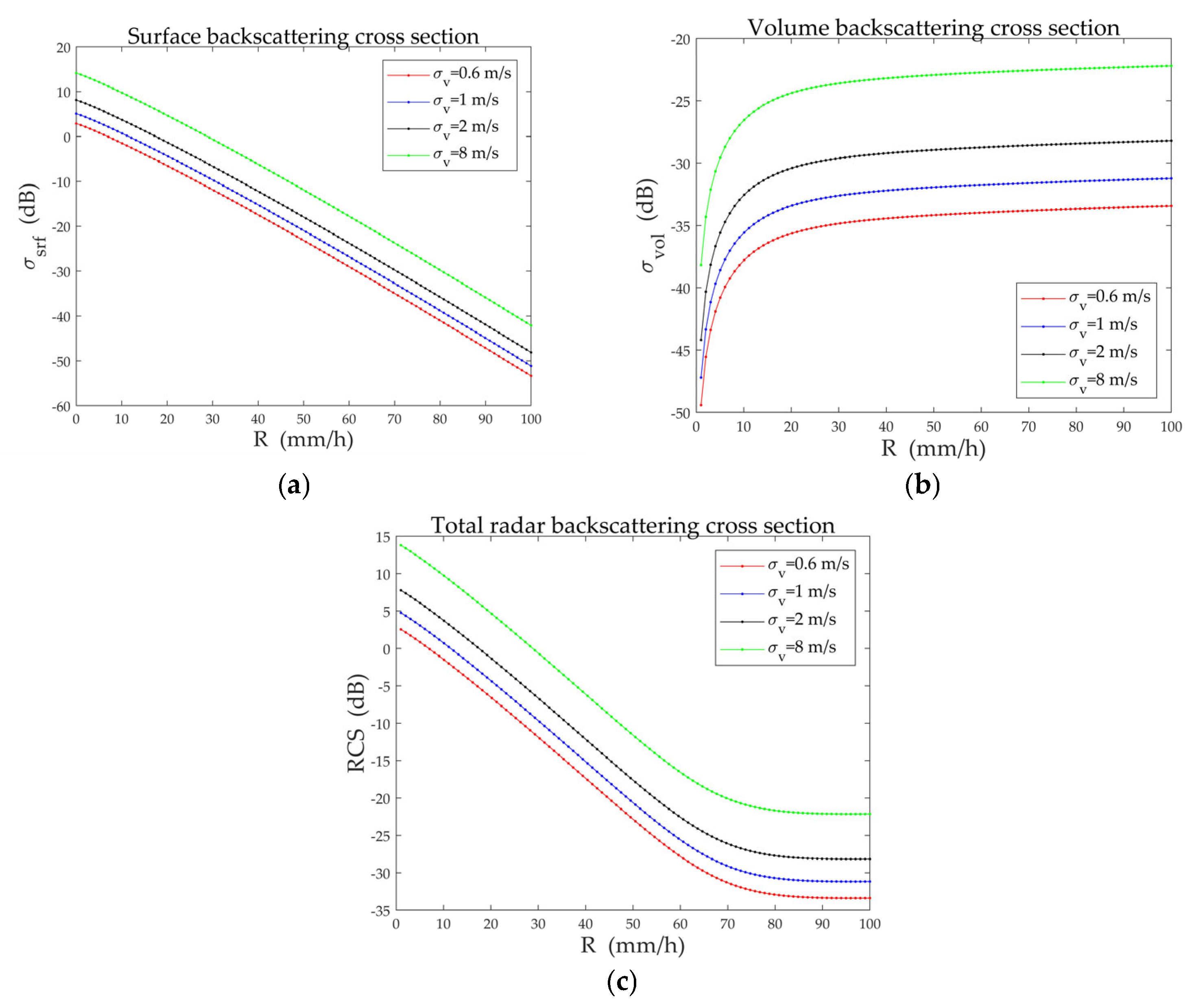
5.1. RCS under Raindrop Motion Error Model

In case 1, we set $h$ = 514 km, $\lambda$ = 3.1 cm, ${\sigma }^0$ = −7 dB, $z_t$ = 13 km, $\theta$ = 30°, and $u$ = 7300 m/s. The precipitation rate $R$ varies from 0 to 100 mm/h, and the standard deviation of the Doppler velocity spectrum of raindrops ${\sigma }_v$ takes values of 0.6 m/s, 1.0 m/s, 2.0 m/s, and 8.0 m/s, respectively. Using Equations (16), (22), and (23), the simulated curves of the surface backscattering cross section ${\sigma }_{srf}$, the volume backscattering cross section ${\sigma }_{vol}$, and the total radar backscattering cross section $\sigma$ with varying $R$ and ${\sigma }_v$ are shown in Figure 5.

Figure 5. Simulation results of RCS. (a) The surface backscattering cross section; (b) The volume backscattering cross section; (c) The total radar backscattering cross section.

Figure 5 shows that the RCS is sensitive to changes in the standard deviation of the raindrop Doppler velocity spectrum. As ${\sigma }_v$ increases under the same precipitation rate, both the area and volume within the effective beam illuminated range increase, leading to a rise in ${\sigma }_{srf}$ and ${\sigma }_{vol}$. Additionally, when ${\sigma }_v$ is 1 m/s and 2 m/s, respectively, the difference between the two sets of ${\sigma }_{srf}$ and ${\sigma }_{vol}$ curves remains constant at 3 dB. The difference is determined by the coefficients of the two parts on the right side of Equation (26), confirming the accuracy of the theoretical analysis. Based on this result, we can conduct the experiments below to examine the impact of raindrop motion on the accuracy of MOS inversion results.

5.2. Retrieval Results of Precipitation Distribution

In this section, the RMM algorithm is used to simulate the inversion results of surface rainfall rate, horizontal distribution, and two-dimensional precipitation distribution under windy and windless conditions, respectively. By comparing these two sets of results, we can evaluate the impact of raindrop motion on inversion accuracy.

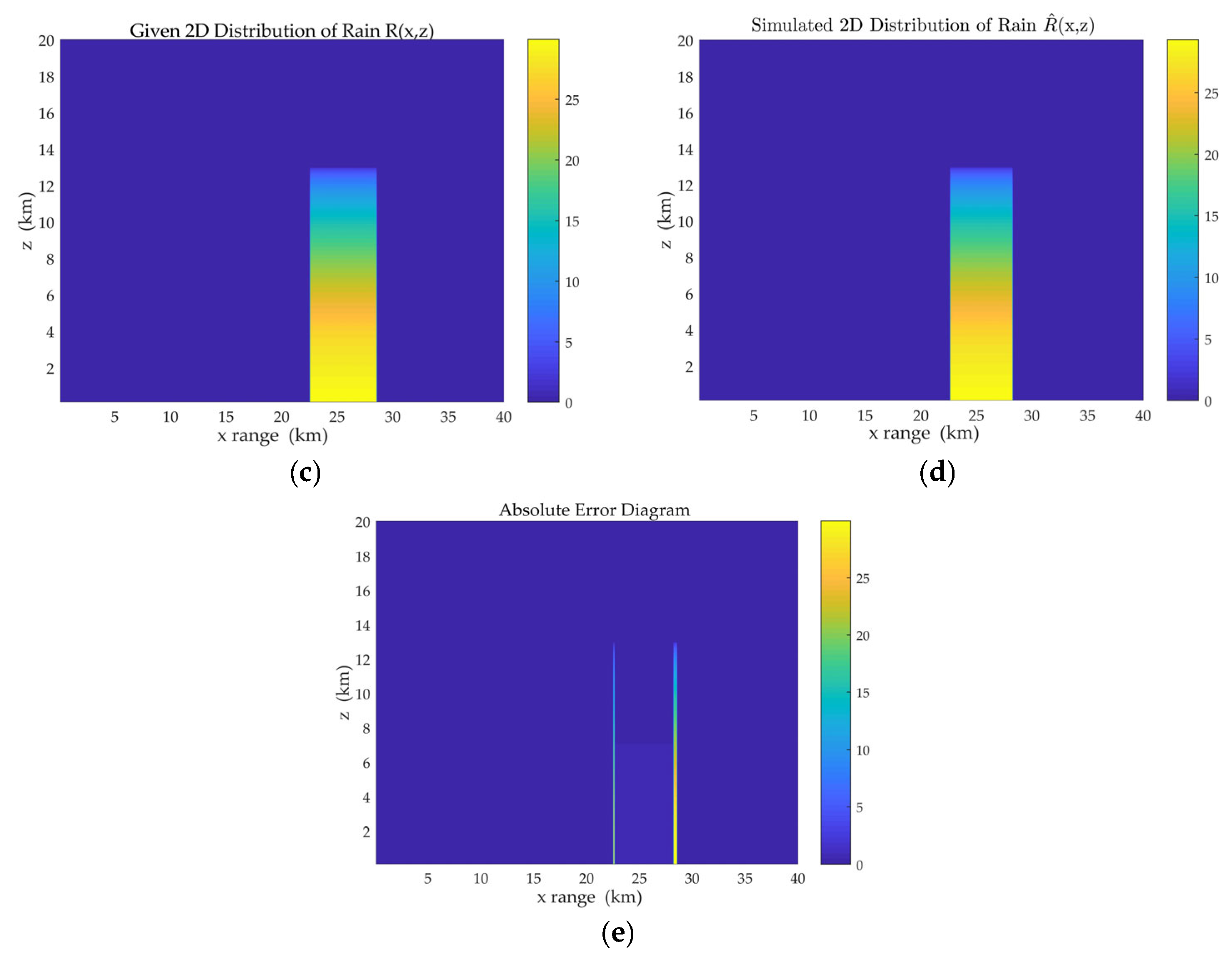
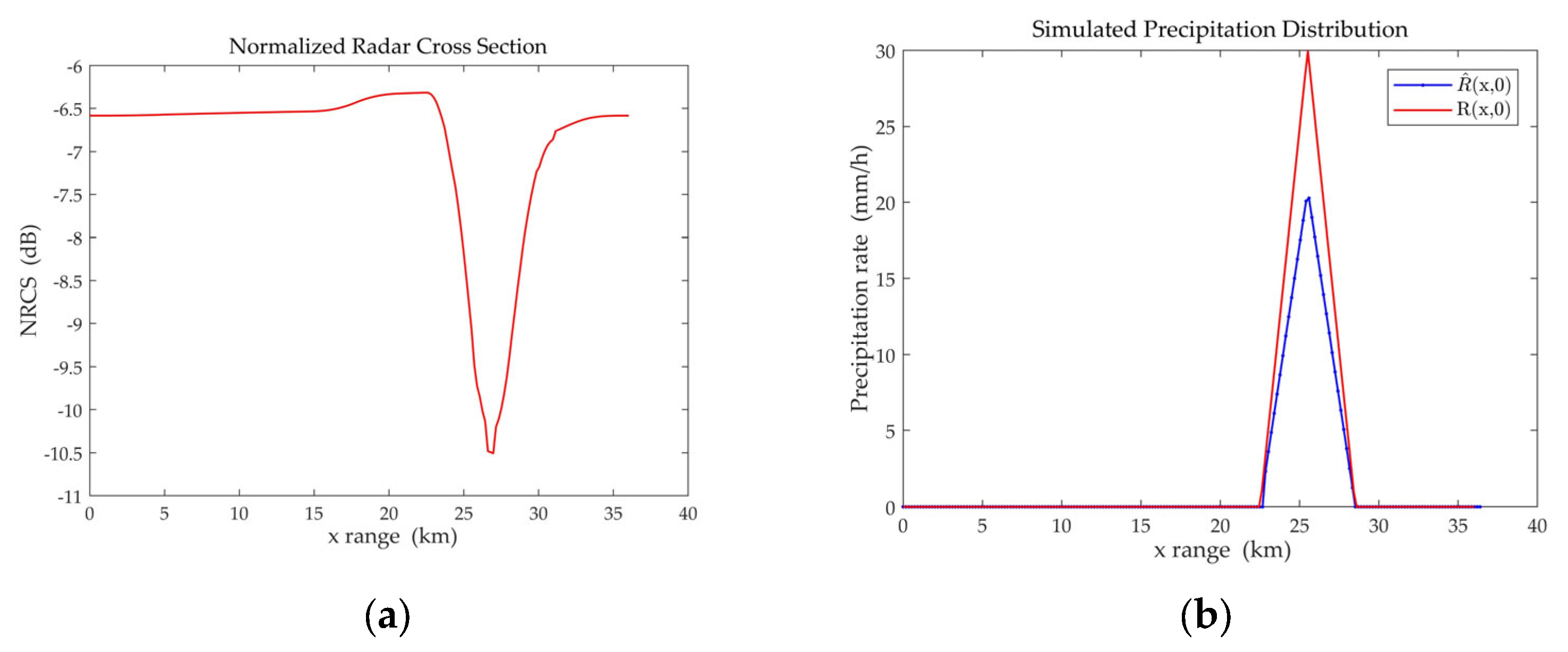
5.2.1. Simulation without Raindrop Motion

When ${\sigma }_v$ = 1 m/s, it means that the raindrop motion error model in Figure 3 is not considered, and the RMM algorithm is simplified to the original MOS algorithm. We first simulate and analyze the retrieval results of the original MOS algorithm with various combinations of rainfall parameters in cases 2–4. We set the relevant parameters of the rainfall area as follows: $w$ = 6 km, $z_0$ = 4.5 km, $z_t$ = 13 km, $\theta$ = 30°, and ${\sigma }^0$ = −7 dB. It is assumed that $R(x,0)$ consists of a horizontal distribution $H\left(x\right)$ and a surface rain rate $V\left(0\right)$:

$$R\left(x,0\right)=H\left(x\right)V\left(0\right)$$

(35)

Case 2: Taking a rectangular rain cloud ($d$ = 0 km), the surface rain rate is 30 mm/h. The NRCS data and the inversion results are shown in Figure 6. The surface rain rate retrieved by RMM of ${\sigma }_v$ = 1 m/s is 29.36 mm/h.

Figure 6. Inversion results under rectangular horizontal distribution by RMM of ${\sigma }_v$ = 1 m/s. (a) The normalized radar cross section; (b) Simulated precipitation distribution $\widehat{R}(x,0)$; (c) Given precipitation distribution $R(x,z)$; (d) Simulated precipitation distribution $\widehat{R}(x,z)$; (e) Absolute error diagram.

Case 3: Taking a trapezoidal rain cloud ($d$ = 1.5 km), the surface rain rate is 30 mm/h. The inversion results are shown in Figure 7. The surface rain rate retrieved by RMM of ${\sigma }_v$ = 1 m/s is 30.94 mm/h.

Figure 7. Trapezoidal distribution diagrams retrieved by RMM of ${\sigma }_v$ = 1 m/s. (a) The normalized radar cross section; (b) Simulated precipitation distribution $\widehat{R}(x,0)$.

Case 4: Taking a triangular rain cloud ($d$ = 3 km), the surface rain rate is 30 mm/h. The inversion results are shown in Figure 8. The surface rain rate retrieved by RMM of ${\sigma }_v$ = 1 m/s is 30.82 mm/h.

Figure 8. Triangular distribution diagrams retrieved by RMM of ${\sigma }_v$ = 1 m/s. (a) The normalized radar cross section; (b) Simulated precipitation distribution $\widehat{R}(x,0)$.

Case 5: Assume that the model surface rain rate varies from 5 to 100 mm/h, and the horizontal precipitation distribution takes rectangular ($d$ = 0 km), trapezoidal ($d$ = 1.5 km), and triangular ($d$ = 3 km) shapes, respectively. Three sets of the retrieved surface rates, each consisting of 20 values, are shown in Figure 9.

Figure 9. Surface rain rate of 5 to 100 mm/h retrieved by RMM of ${\sigma }_v$ = 1 m/s.

Case 6: Assume that the model surface rain rate varies from 20 to 40 mm/h, and the horizontal precipitation distribution takes rectangular ($d$ = 0 km), trapezoidal ($d$ = 1.5 km), and triangular ($d$ = 3 km) shapes, respectively. Three sets of the retrieved surface rates, each consisting of 21 values, are shown in Figure 10.

Figure 10. Surface rain rate of 20 to 40 mm/h retrieved by RMM of ${\sigma }_v$ = 1 m/s.

Figure 6e shows the absolute error between the retrieved two-dimensional precipitation distribution $\widehat{R}(x,z)$ and the given two-dimensional precipitation distribution $R(x,z)$. More significant absolute errors occur at the edges of the rainfall area. This is mainly because of the error in the retrieved rainfall area width $\widehat{w}$. Furthermore, the MOS can be applied to rain clouds of various shapes, as shown in Figure 6, Figure 7 and Figure 8. This method can also be applied to various rainfall rates, as shown in Figure 9 and Figure 10. The above results prove that the retrieval results using the MOS are in good agreement with the given rain cloud model in windless conditions, where the impact of raindrop motion error is negligible.

In Figure 9, the MOS exhibits a better inversion effect during moderate to heavy rainfall. Consequently, our subsequent research will primarily focus on experiments where the surface rain rate ranges from 20 to 40 mm/h.

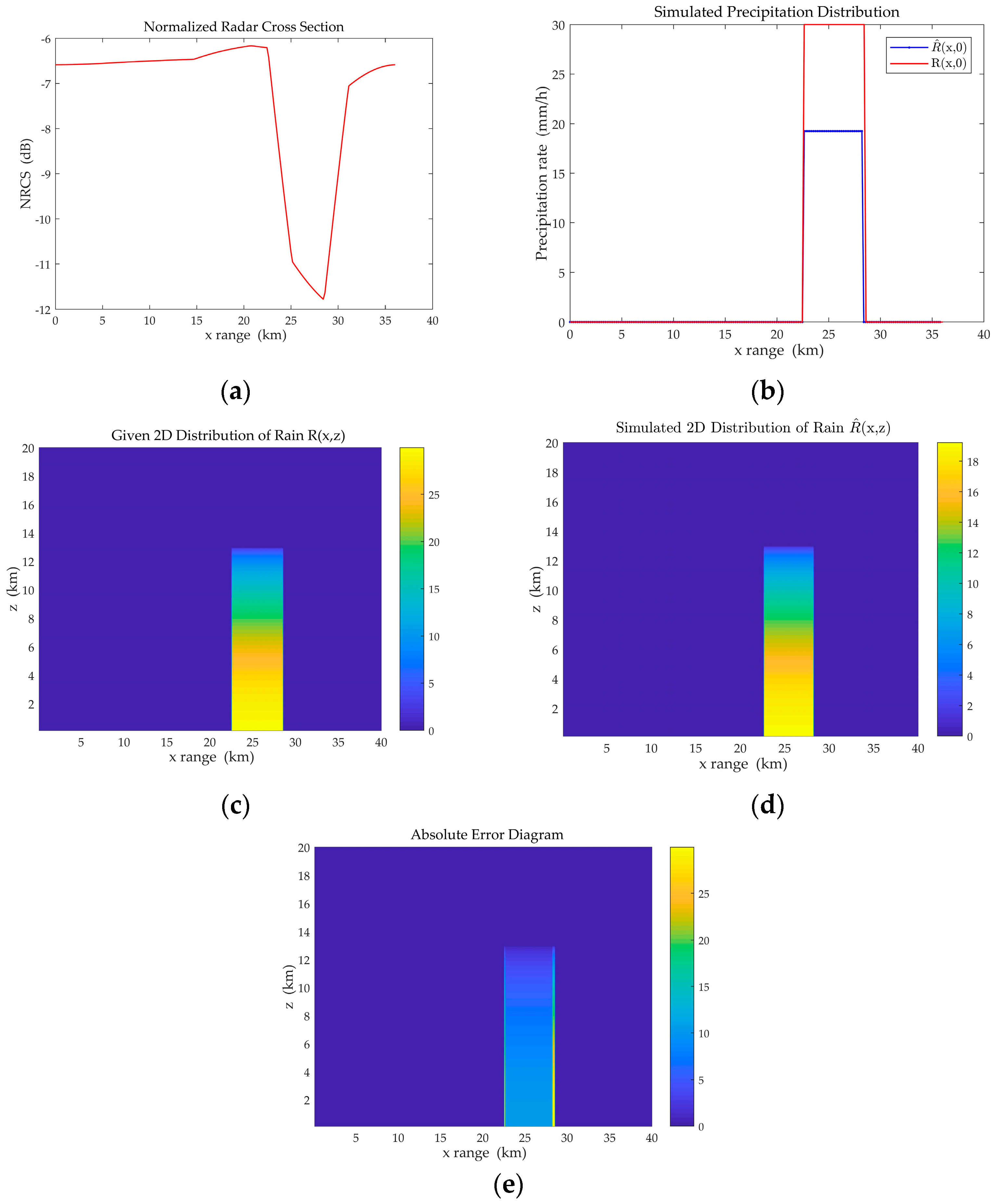
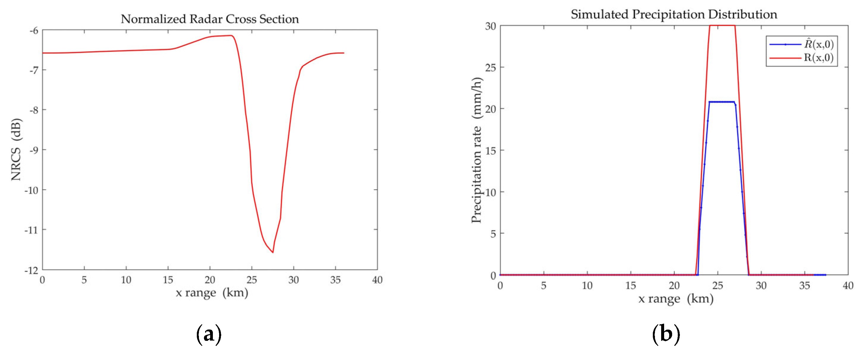
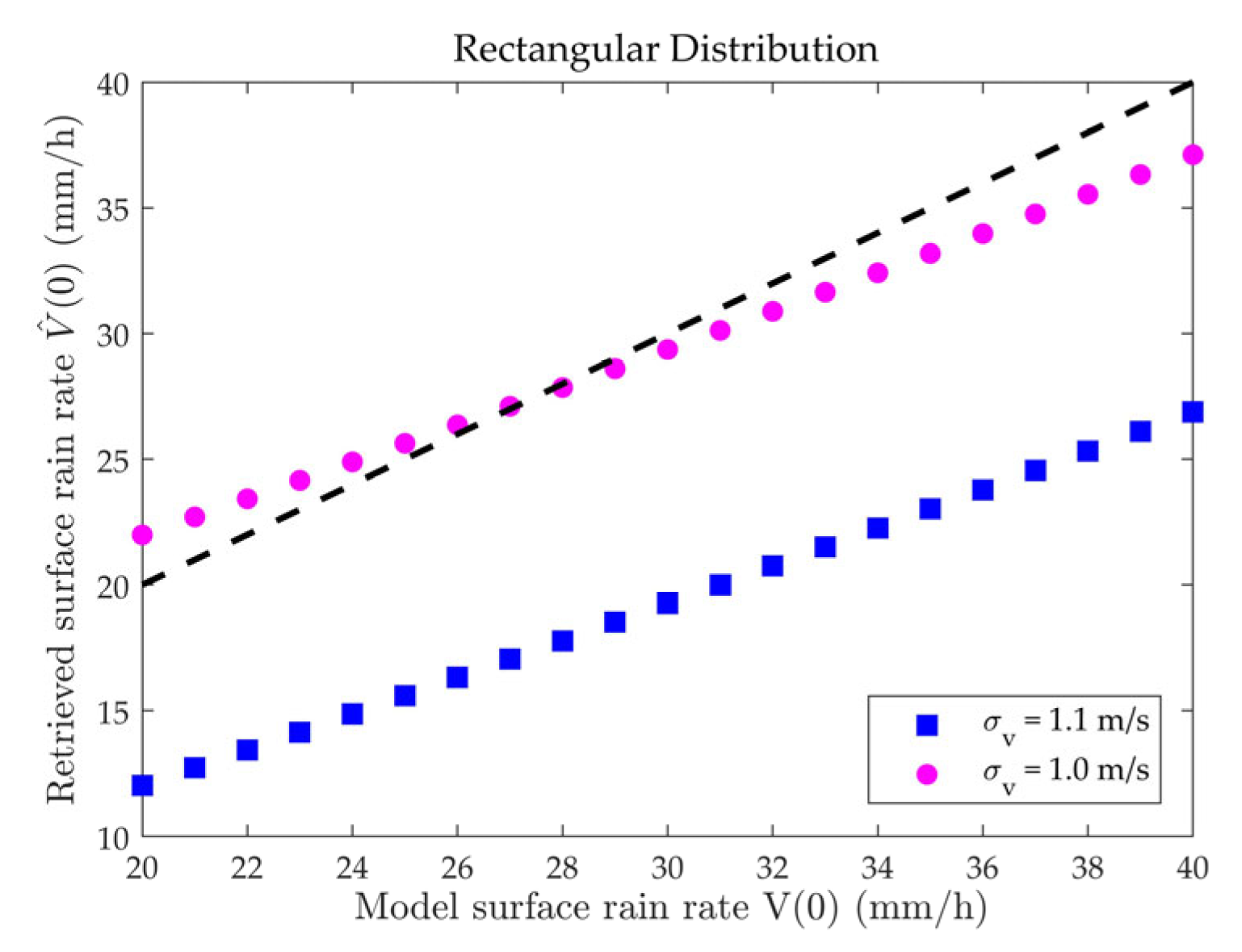
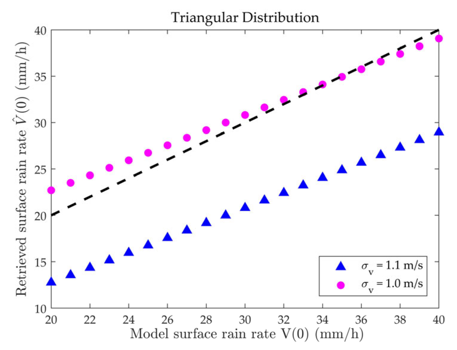
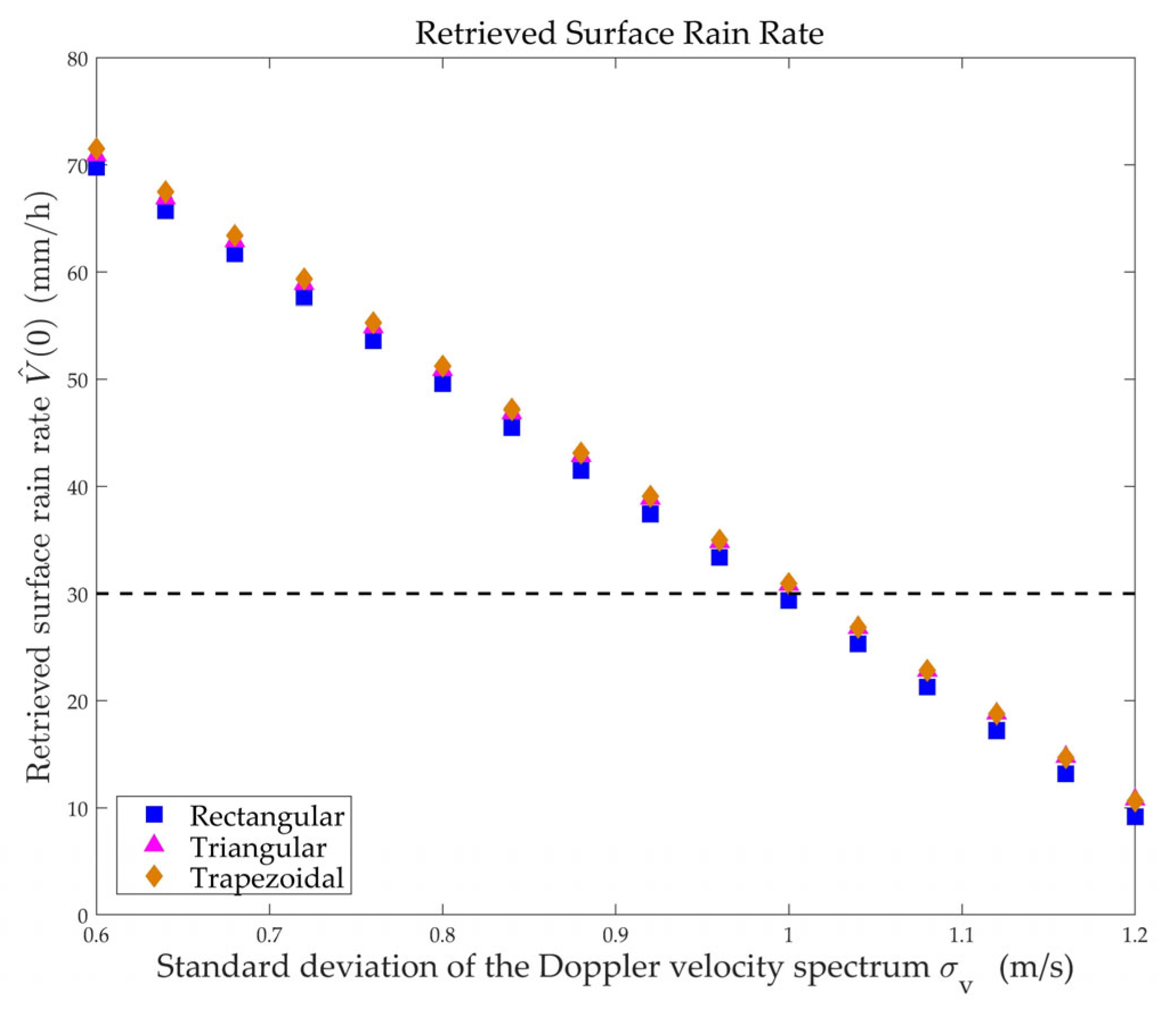
5.2.2. Simulation with Raindrop Motion

In Figure 5, the experimental results show the RCS with raindrop motion error that, according to Equation (26), can be converted to NRCS data. These data are then used for precipitation inversion. For a fixed surface rain rate, we use the RMM algorithm to evaluate the inversion error caused by raindrop motion in cases 7–9. In cases 10–12, we compare inversion results under a range of surface rain rates, consisting of 21 values, to better illustrate the motion error’s impact on the retrieved surface rain rate. Case 13 further explores the variances in retrieved surface rain rates for different standard deviations of the raindrop Doppler velocity spectrum.

Case 7: Taking a rectangular rain cloud, ${\sigma }_v$ is 1.1 m/s, and the surface rain rate is 30 mm/h. The inversion results of RMM are shown in Figure 11. The surface rain rate retrieved by RMM is 19.26 mm/h.

Figure 11. Inversion results under rectangular horizontal distribution by RMM of ${\sigma }_v$ = 1.1 m/s. (a) The normalized radar cross section; (b) Simulated precipitation distribution $\widehat{R}(x,0)$; (c) Given precipitation distribution $R(x,z)$; (d) Simulated precipitation distribution $\widehat{R}(x,z)$; (e) Absolute error diagram.

Case 8: Taking a trapezoidal rain cloud, ${\sigma }_v$ is 1.1 m/s, and the surface rain rate is 30 mm/h. The inversion results of RMM are shown in Figure 12. The surface rain rate retrieved by RMM is 20.79 mm/h.

Figure 12. Trapezoidal distribution diagrams retrieved by RMM of ${\sigma }_v$ = 1.1 m/s. (a) The normalized radar cross section; (b) Simulated precipitation distribution $\widehat{R}(x,0)$.

Case 9: Taking a triangular rain cloud, ${\sigma }_v$ is 1.1 m/s, and the surface rain rate is 30 mm/h. The inversion results of RMM are shown in Figure 13. The surface rain rate retrieved by RMM is 20.80 mm/h.

Figure 13. Triangular distribution diagrams retrieved by RMM of ${\sigma }_v$ = 1.1 m/s. (a) The normalized radar cross section; (b) Simulated precipitation distribution $\widehat{R}(x,0)$.

Case 10: Taking a rectangular rain cloud, the surface rain rate varies from 10 to 50 mm/h, and ${\sigma }_v$ takes 1 m/s and 1.1 m/s, respectively. The surface rain rates retrieved by RMM are shown in Figure 14.

Figure 14. Scatterplot of surface rain rates retrieved by RMM under rectangular horizontal distribution.

Case 11: Taking a trapezoidal rain cloud, the surface rain rate varies from 10 to 50 mm/h, and ${\sigma }_v$ takes 1 m/s and 1.1 m/s, respectively. The surface rain rates retrieved by RMM are shown in Figure 15.

Figure 15. Scatterplot of surface rain rates retrieved by RMM under trapezoidal horizontal distribution.

Case 12: Taking a triangular rain cloud, the surface rain rate varies from 10 to 50 mm/h, and ${\sigma }_v$ takes 1 m/s and 1.1 m/s, respectively. The surface rain rates retrieved by RMM are shown in Figure 16.

Figure 16. Scatterplot of surface rain rates retrieved by RMM under triangular horizontal distribution.

Several groups of the retrieved surface rainfall data are selected for an error analysis. The relative error (RE) of the surface rain rate is as follows:

$$RE=\left|\frac{\widehat{V}\left(0\right)-V\left(0\right)}{V\left(0\right)}\right|$$

(36)

The root mean square error (RMS) of the surface rain rate is as follows:

$$RM{S}_n=\sqrt{\frac{1}{n}\sum _{i=1}^n{\left[\frac{{\widehat{V}\left(0\right)}_i-{V\left(0\right)}_i}{{V\left(0\right)}_i}\right]}^2}$$

(37)

The attributes of the six selected cases are shown in Table 1, and Table 2 shows the relative error for these cases. Table 3 shows the root mean square error of the cases 10–12.

Table 1. The attributes of the 6 cases.

	$\mathit{V}\left(0\right) (\mathbf{m}\mathbf{m}/\mathbf{h})$	${\mathit{\sigma }}_{\mathit{v}} (\mathbf{m}/\mathbf{s})$	$\mathit{w} \left(\mathbf{k}\mathbf{m}\right)$	Shape of Rain Cloud(s)
Case 2	30	1.0	6	Rectangular
Case 3	30	1.0	6	Trapezoidal
Case 4	30	1.0	6	Triangular
Case 7	30	1.1	6	Rectangular
Case 8	30	1.1	6	Trapezoidal
Case 9	30	1.1	6	Triangular

Table 2. Analysis of relative error of the cases.

	$\widehat{\mathit{V}}\left(0\right) (\mathbf{m}\mathbf{m}/\mathbf{h})$	$\mathit{R}\mathit{E}$ (%)	$\widehat{\mathit{w}} \left(\mathbf{k}\mathbf{m}\right)$	Shape of Rain Cloud(s)
Case 2	29.36	2.13	5.62	Rectangular
Case 3	30.94	3.13	7.06	Trapezoidal
Case 4	30.82	2.73	6.07	Triangular
Case 7	19.26	35.80	5.62	Rectangular
Case 8	20.79	30.70	7.06	Trapezoidal
Case 9	20.80	30.67	6.07	Triangular

Table 3. Root mean square error of the cases 10–12.

	${\mathit{\sigma }}_{\mathit{v}}=1.0 \mathbf{m}/\mathbf{s}$	${\mathit{\sigma }}_{\mathit{v}}=1.1 \mathbf{m}/\mathbf{s}$	Shape of Rain Cloud(s)
Case 10	0.052	0.361	Rectangular
Case 11	0.047	0.318	Trapezoidal
Case 12	0.060	0.312	Triangular

Case 13: Assume that the standard deviation of the raindrop Doppler velocity spectrum ranges from 0.6 to 1.2 m/s, the surface rain rate is 30 mm/h, and the horizontal distribution of precipitation takes rectangular (d = 0 km), trapezoidal (d = 1.5 km), and triangular (d = 3 km) shapes, respectively. Three sets of the retrieved surface rates, each consisting of 20 values, are shown in Figure 17.

Figure 17. Surface rain rates of ${\sigma }_v$ ranging from 0.6 to 1.2 m/s retrieved by RMM.

Taking cases 2–4 as the control group, cases 7–9 can provide insight into the inversion errors caused by raindrop motion in the MOS algorithm. Taking the rectangular rain cloud as an example, it can be observed from Figure 6a and Figure 11a that the NRCS curve corresponding to ${\sigma }_v$ = 1.1 m/s is approximately 0.4 dB higher than the original NRCS curve. Comparing Figure 6e and Figure 11e, it can be observed that raindrop motion also introduces significant errors to the retrieved two-dimensional precipitation distribution $\widehat{R}(x,z)$, which are beyond the acceptable error range. For the inversion of surface rain rate, under a rectangular rain cloud with ${\sigma }_v$ = 1.1 m/s and $V\left(0\right)$ = 30 mm/h, the relative error of $\widehat{V}(0)$ increases from the original 2.13% to 35.80% in Table 2. Similar conclusions also apply to trapezoidal and triangular rain clouds. The ${RMS}_{21}$ under the three different shapes of the rain clouds are very close to each other in Table 3. The ${RMS}_{21}$ of ${\sigma }_v$ = 1.0 m/s is approximately 0.05, but the ${RMS}_{21}$ of ${\sigma }_v$ = 1.1 m/s increases to approximately 0.32. The results above show that the inversion accuracy of MOS is significantly affected after introducing different raindrop motion errors.

In Figure 14, Figure 15 and Figure 16, the curve of retrieved surface rain rates $\widehat{V}(0)$ noticeably decreases when ${\sigma }_v$ is greater than 1 m/s. Figure 17 provides a clearer view of how retrieved surface rain rates change with ${\sigma }_v$ under three different precipitation distributions. Taking ${\sigma }_v$ = 1 m/s as the dividing line, the two sides of the horizontal axis represent the introduction of varying levels of raindrop motion errors. The value of $\widehat{V}(0)$ increases when ${\sigma }_v$ is less than 1 m/s and decreases when ${\sigma }_v$ is larger than 1 m/s. Moreover, the degree of deviation from $V\left(0\right)$ in $\widehat{V}(0)$ is related to the extent of deviation from 1 m/s in ${\sigma }_v$.

6. Conclusions

In Section 3, we establish the raindrop motion error model and analyze the RCS under different raindrop Doppler velocity spectrum standard deviations to identify the RCS’s variation pattern. In this way, the relationship between the wind field, raindrop motion, and SAR echoes is established. When ${\sigma }_v$ takes 1 m/s and 2 m/s, respectively, the difference between the two groups of ${\sigma }_{srf}$ and ${\sigma }_{vol}$ remains constant with a total RCS difference of 3 dB. Next, the RMM algorithm is proposed, based on the raindrop motion error model. This algorithm allows for us to examine the impact of raindrop motion on the original MOS inversion model and accurately calculate the resulting error in precipitation retrieval. In the RMM algorithm, introducing the raindrop motion error increases the relative error of the retrieved surface rain rate $\widehat{V}(0)$ from the original 2.13% to 35.80% under a rectangular rain cloud with ${\sigma }_v$ = 1.1 m/s and $V\left(0\right)$ = 30 mm/h. The degree to which the retrieved surface rain rate differs from the given one is strongly correlated with the value of ${\sigma }_v$. The inversion error significantly increases, indicating that the impact of raindrop motion on the accuracy of the MOS algorithm cannot be neglected. The current inversion algorithms, such as the MOS, require modifications to the relevant retrieval models when a wind field is present in the rainfall environment.

The original MOS algorithm does not account for wind fields influencing raindrops in actual rainfall environments. Therefore, in conjunction with the analysis and simulation in this paper, we suggest adding a motion compensation module to further improve the accuracy and applicability of the MOS algorithm. The problem becomes tractable when we obtain the standard deviation of the Doppler velocity spectrum in actual precipitation measurements. Adding a data preprocessing step to the MOS can rectify the impact of wind-induced raindrop motion on SAR rainfall retrieval accuracy.

This study provides a preliminary understanding of the theoretical framework regarding how raindrop motion impacts the MOS inversion error, using the standard deviation of the Doppler velocity spectrum of raindrops ${\sigma }_v$. We have made some simplifications to the rain motion model and the double-layer rain cloud model. Naturally, the variation in ${\sigma }_v$ itself, influenced by environmental wind field velocities, is a highly complex process with many error factors. In the actual atmosphere, wind speed and direction vary with altitude [41]. In turbulent air, particles of a certain diameter within the effective illuminated volume not only fall at speeds influenced by environmental wind and gravity but also move with the surrounding atmospheric turbulent [42]. Further research could consider several aspects, such as the observation and modelling of the background wind field, the motion characteristics of raindrops within the wind field, and the acquisition of raindrop spectrum distribution data. Therefore, a more comprehensive study needs to focus on developing a refined correlation between wind field, wind speed, and the standard deviation of the Doppler velocity spectrum of raindrops and studying intricate rainfall distributions in more realistic situations. This paper’s research findings can provide a certain reference for rainfall inversion, taking into account the error of raindrop motion.

References

- Skofronick-Jackson, G.M.; Draper, D.W.; Newell, D.A. The Global Precipitation Measurement (GPM) Mission. In Proceedings of the IGARSS 2020—2020 IEEE International Geoscience and Remote Sensing Symposium, Waikoloa, HI, USA, 26 September–2 October 2020; pp. 3589–3592. [Google Scholar]
- Huffman, G.J.; Bolvin, D.T.; Nelkin, E.J.; Wolff, D.B.; Adler, R.F.; Gu, G.; Hong, Y.; Bowman, K.P.; Stocker, E.F. The TRMM Multisatellite Precipitation Analysis (TMPA): Quasi-global, Multiyear, Combined-sensor Precipitation Estimates at Fine Scales. J. Hydrometeorol. 2007, 8, 38–55. [Google Scholar] [CrossRef]
- Huffman, G.; Bolvin, D.; Braithwaite, D.; Hsu, K.; Joyce, R.; Kidd, C.; Nelkin, E.; Xie, P. NASA Global Precipitation Measurement Integrated Multi-Satellite Retrievals for GPM (IMERG). Algorithm Theoretical Basis Doc.; Version 4.5; National Aeronautics and Space Administration: Washington, DC, USA, 2015; 30p. [Google Scholar]
- Eineder, M.; Minet, C.; Steigenberger, P.; Cong, X.Y.; Fritz, T. Imaging Geodesy-toward Centimeter-level Ranging Accuracy with TerraSAR-X. IEEE Trans. Geosci. Remote Sens. 2011, 49, 661–671. [Google Scholar] [CrossRef]
- Chen, J.; Jia, H.F.; Yang, J.; Chen, Y.R. Primary Exploration on Monitoring of River Pollution Based on Polarimetric Coherence Matrix. J. Remote Sens. 2011, 15, 1065–1078. [Google Scholar] [CrossRef]
- Wu, T.; Wang, C.; Zhang, H.; Zhang, Z.X. Space-borne SAR Image Simulation Based on Image Characteristics. J. Remote Sens. 2007, 11, 214–220. [Google Scholar] [CrossRef]
- Navarro, A.; García-Ortega, E.; Merino, A.; Sánchez, J.L.; Tapiador, F.J. Orographic Biases in IMERG Precipitation Estimates in the Ebro River Basin (Spain): The Effects of Rain Gauge Density and Altitude. Atmos. Res. 2020, 244, 10. [Google Scholar] [CrossRef]
- Leng, X.G.; Ji, K.F.; Kuang, G.Y. Ship Detection from Raw SAR Echo Data. IEEE Trans. Geosci. Remote Sens. 2023, 61, 11. [Google Scholar] [CrossRef]
- Duysak, H.; Yigit, E. Investigation of the Performance of Different Wavelet-based Fusions of SAR and Optical Images Using Sentinel-1 and Sentinel-2 Datasets. Int. J. Eng. Geosci. 2022, 7, 81–90. [Google Scholar] [CrossRef]
- Jackson, C. Synthetic Aperture Radar: Marine User’s Manual; United States Government Printing Office: Washington, DC, USA, 2004; pp. 1–25. [Google Scholar]
- Jameson, A.R.; Li, F.K.; Durden, S.L.; Haddad, Z.S.; Holt, B.M.; Fogarty, T.; Im, E.; Moore, R.K. SIR-C/X-SAR Observations of Rain Storms. Remote Sens. Environ. 1997, 59, 267–279. [Google Scholar] [CrossRef]
- Hou, A.Y.; Kakar, R.K.; Neeck, S.; Azarbarzin, A.A.; Kummerow, C.D.; Kojima, M.; Oki, R.; Nakamura, K.; Iguchi, T. The Global Precipitation Measurement Mission. Bull. Amer. Meteorol. Soc. 2014, 95, 701–722. [Google Scholar] [CrossRef]
- Melsheimer, C.; Alpers, W.; Gade, M. Investigation of Multifrequency/Multipolarization Radar Signatures of Rain Cells over the Ocean Using SIR-C/X-SAR Data. J. Geophys. Res. Ocean. 1998, 103, 18867–18884. [Google Scholar] [CrossRef]
- Moore, R.K.; Mogili, A.; Fang, Y.; Beh, B.; Ahamad, A. Rain Measurement with SIR-C/X-SAR. Remote Sens. Environ. 1997, 59, 280–293. [Google Scholar] [CrossRef]
- Pichugin, A.P.; Spiridonov, Y.G. Spatial-distribution of Rainfall Intensity Recovery from Space Radar Images. Sov. J. Remote Sens. 1991, 8, 917–932. [Google Scholar]
- Weinman, J.A.; Marzano, F.S. An Exploratory Study to Derive Precipitation over Land from X-band Synthetic Aperture Radar Measurements. J. Appl. Meteorol. Climatol. 2008, 47, 562–575. [Google Scholar] [CrossRef]
- Weinman, J.A.; Marzano, F.S.; Plant, W.J.; Mugnai, A.; Pierdicca, N. Rainfall Observation from X-band Spaceborne Synthetic Aperture Radar. Nat. Hazards Earth Syst. Sci. 2009, 9, 77–84. [Google Scholar] [CrossRef]
- Zheng, Y.; Shi, Z.; Lu, Z.Z.; Ma, W.F. A Method for Detecting Rainfall From X-Band Marine Radar Images. IEEE Access 2020, 8, 19046–19057. [Google Scholar] [CrossRef]
- Zhao, Y.; Longépé, N.; Mouche, A.; Husson, R. Automated Rain Detection by Dual-Polarization Sentinel-1 Data. Remote Sens. 2021, 13, 3155. [Google Scholar] [CrossRef]
- Draper, D.W.; Long, D.G. Evaluating the Effect of Rain on SeaWinds Scatterometer Measurements. J. Geophys. Res. Ocean. 2004, 109, 12. [Google Scholar] [CrossRef]
- Satake, M.; Matsuoka, T.; Kobayashi, T.; Kojima, S.; Uemoto, J.; Umehara, T.; Uratsuka, S.; Yamaguchi, Y. Polarimetric Data Analysis of a Rainfall Event Observed by X-band Airborne SAR. In Proceedings of the IGARSS 2014—2014 IEEE International Geoscience and Remote Sensing Symposium, Quebec, QC, Canada, 13–18 July 2014; pp. 4105–4106. [Google Scholar]
- YU, S.; Yang, J.S.; He, S.Y.; He, Z.G.; Zheng, G. The Correction of Rain Effect on SAR Wind Field Retrieval. Haiyang Xuebao 2017, 39, 11. [Google Scholar] [CrossRef]
- Shen, H.; Seitz, C.; Perrie, W.; He, Y.J.; Powell, M. Developing a Quality Index Associated with Rain for Hurricane Winds from SAR. Remote Sens. 2018, 10, 1783. [Google Scholar] [CrossRef]
- Shao, W.Z.; Lai, Z.Z.; Nunziata, F.; Buono, A.; Jiang, X.W.; Zuo, J.C. Wind Field Retrieval with Rain Correction from Dual-Polarized Sentinel-1 SAR Imagery Collected during Tropical Cyclones. Remote Sens. 2022, 14, 5006. [Google Scholar] [CrossRef]
- Xu, F.; Li, X.F.; Jin, Y.Q. Physics-based Scattering Model of Rainfall over Sea Surface. In Proceedings of the 29th URSI General Assembly and Scientific Symposium (URSI GASS), Beijing, China, 16–23 August 2014; pp. 1–4. [Google Scholar]
- Zhang, P.C.; Du, B.Y.; Dai, T.P. Radar Meteorology, 2nd ed.; China Meteorological Press: Beijing, China, 2001; pp. 1–50. [Google Scholar]
- Probert-Jones, J.R. The Radar Equation in Meteorology. Q. J. Roy. Meteor. Soc. 1962, 88, 485–495. [Google Scholar] [CrossRef]
- Ahamad, A. Limitation on the Use of a Spaceborne SAR for Rain Measurements. NASA STI Recon Tech. Rep. N 1994, 95, 11228. [Google Scholar]
- Olsen, R.L.; Rogers, D.V.; Hodge, D.B. The aRb Relation in the Calculation of Rain Attenuation. IEEE Trans. Antennas Propag. 1978, 26, 318–329. [Google Scholar] [CrossRef]
- Sekhon, R.S.; Srivastava, R.C. Doppler Radar Observations of Drop-size Distributions in a Thunderstorm. J. Atmos. Sci. 1971, 28, 983–994. [Google Scholar] [CrossRef]
- Ulaby, F.T.; Moore, R.K.; Fung, A.K. Microwave Remote Sensing: Active and Passive, 3rd ed.; Addison-Wesley Pub. Co.: London, UK, 1981; pp. 318–328. [Google Scholar]
- Long, T.; Ding, Z.G.; Xiao, F.; Wang, Y.; Li, Z. Spaceborne High-resolution Stepped-frequency SAR Imaging Technology. J. Radars 2019, 8, 782–792. [Google Scholar] [CrossRef]
- Atlas, D.; Moore, R.K. The Measurement of Precipitation with Synthetic Aperture Radar. J. Atmos. Ocean. Technol. 1987, 4, 368–376. [Google Scholar] [CrossRef]
- Li, N.N.; Zhou, M.L.; Xie, Y.N. An Effective Echo Method for Precipitation Measurement by SAR at Different Doppler Velocities. Ind. Control Comput. 2018, 31, 3. [Google Scholar] [CrossRef]
- Oh, Y.; Sarabandi, K.; Ulaby, F.T. An Empirical Model and an Inversion Technique for Radar Scattering from Bare Soil Surfaces. IEEE Trans. Geosci. Remote Sens. 1992, 30, 370–381. [Google Scholar] [CrossRef]
- Tang, J.; Chen, S.; Li, Z.; Gao, L. Mapping the Distribution of Summer Precipitation Types over China Based on Radar Observations. Remote Sens. 2022, 14, 3437. [Google Scholar] [CrossRef]
- Xie, Y.N.; Huan, J.P. Feasibility Analysis of Spaceborne SAR Measuring Precipitation. In Proceedings of the Chinese Meteorological Society Meeting in 2008 of the Satellite Remote Sensing Technology and Treatment Methods Session, Beijing, China, 19–22 November 2008; pp. 265–269. [Google Scholar]
- Marzano, F.S.; Weinman, J.A. Inversion of Spaceborne X-band Synthetic Aperture Radar Measurements for Precipitation Remote Sensing Over Land. IEEE Trans. Geosci. Remote Sens. 2008, 46, 3472–3487. [Google Scholar] [CrossRef]
- Luo, T.; Xie, Y.N.; Wang, R.; Yu, X.Y. An Analytic Solution to Precipitation Attenuation Expression with Spaceborne Synthetic Aperture Radar Based on Volterra Integral Equation. Remote Sens. 2022, 14, 357. [Google Scholar] [CrossRef]
- Xie, Y.N.; Liu, Z.K.; An, D.W. An Algorithm to Retrieve Precipitation with Synthetic Aperture Radar. J. Meteorol. 2016, 30, 401–411. [Google Scholar] [CrossRef]
- Wu, Y.Y.; Li, Q.L.; Li, G.X.; He, B.; Dong, L.; Lang, H.N.; Zhang, L.J.; Chen, S.P.; Tang, X.X. Vertical Wind Speed Variation in a Metropolitan City in South China. Earth Space Sci. 2022, 9, 20. [Google Scholar] [CrossRef]
- Testik, F.Y.; Boleka, A. Wind and Turbulence Effects on Raindrop Fall Speed. J. Atmos. Sci. 2023, 80, 1065–1086. [Google Scholar] [CrossRef]
Disclaimer/Publisher’s Note: The statements, opinions and data contained in all publications are solely those of the individual author(s) and contributor(s) and not of MDPI and/or the editor(s). MDPI and/or the editor(s) disclaim responsibility for any injury to people or property resulting from any ideas, methods, instructions or products referred to in the content. |
© 2024 by the authors. Licensee MDPI, Basel, Switzerland. This article is an open access article distributed under the terms and conditions of the Creative Commons Attribution (CC BY) license (https://creativecommons.org/licenses/by/4.0/).