Spline Model: A Hydrostatic/Non-Hydrostatic Dynamic Core with Space-Time Second-Order Precision and Its Exact Tests

Abstract

We present a new explicit quasi-Lagrangian integration scheme with the three-dimensional cubic spline function transform (transform = fitting + interpolation, referred to as the “spline format”) on a spherical quasi-uniform longitude–latitude grid. It is a consistent longitude–latitude grid, and to verify the feasibility, accuracy, convergence, and stability of the spline format interpolation scheme for the upstream point on the longitude–latitude grid, which may map a quasi-uniform longitude–latitude grid, a set of ideal, exact test schemes is adopted, which are recognized and proven to be effective internationally. The equilibrium flow test, cross-polar flow test, and Rossby–Haurwitz wave test are used to illustrate the spline scheme uniformity to the linear scheme and to overcome the over-dense grid in the polar region and the non-singularity of the poles. The cross-polar flow test demonstrates that the geostrophic wind crosses the polar area correctly, including the South Pole and North Pole. A non-hydrostatic, fully compressible dynamic core is used to complete the density flow test, demonstrating the existence of a time-varying reference atmosphere and that the spline format can simulate highly nonlinear fine-scale transient flows. It can be compared for the two results of the density flow test between the solution with the spline format and the benchmark reference solution with the linear format. Based on the findings, the non-hydrostatic dynamic core with the spline format is recommended for adoption. When simulated for the flow over an ideal mountain, through the “topographic gravity wave test”, the bicubic surface terrain and terrain-following height coordinates, time-split integration, and vector discrete decomposition can be derived successfully. These may serve as the foundations for a global, unified spline-format numerical model in the future.

1. Introduction

Our paper suggests that by using the cubic spline function, we can build a dynamic framework of numerical modeling based on spatiotemporal second-order precision prediction equations, and then complete a global static/non-static, multi-nested weather prediction numerical model. This should be the development direction of the so-called “Difference Model”. Moreover, using the “line, surface, and volume” cubic spline function to fit three-dimensional variable fields (such as pressure, temperature, or wind), so these become second-order differentiable continuous fields, means that we can replace “discrete Fourier transform” with “continuous Fourier transform” in the Spectral Model. This offers an effective method to improve the calculation accuracy of the Spectral Model and reduce the computational workload.

Many countries (i.e., the US, UK, Japan, Canada, and China) have developed plans to establish globally/regionally unified grid mesh numerical models with horizontal resolutions of 1–100 km. However, the global grid point model’s forecast level has yet to outperform the currently widely adopted global Spectral Model. In recent years, there has been a consensus on how to develop a numerical model system of weather forecasting. It is ranked in order of importance as follows: dynamic core–physical processes (radiation parameterization, cumulus convection parameterization, land surface processes), data assimilation (initial value field, four-dimensional variation), diagnostic analysis, and software support (parallel computing, graphical imaging). The dynamic framework of current numerical models, including the Difference Model and the Spectral Model, has the time integration scheme with less than second-order spatiotemporal accuracy, and its spherical grid scheme, terrain scheme, and reference atmosphere scheme are all under study and improvement.

The mathematical foundation of the Spectral Model is a two-dimensional spectral (spherical harmonics) expansion, which calculates the horizontal upstream point “analytically”, whereas the grid point model generally uses some cubic function interpolation to calculate the upstream point. Such an approach raises a simple question: Is it possible for the cubic function model to outperform the Spectral Model?

Furthermore, we must ask ourselves the following: What mathematical function should be used to fit a physical field as an unknown “primitive function”? First, let us look at pure mathematics.

It is known that two-dimensional spectral expansion is only “convergent” and can achieve “optimal” least square error. However, the spectrum has a few mathematical shortcomings: (1) the horizontal vector field of the spectrum is mathematically singular at the poles (i.e., the spectral model does not forecast for the poles); (2) there are spurious peaks in the plane (termed the “Gibbs phenomenon”); (3) the spectrum is not suitable for the vertical format, fitting neither the upper/lower nor side boundaries, and thus is not suitable to be the global uniform numerical model; and finally, (4) the spectra calculation effort increases rapidly as resolution increases.

There are two types of cubic function interpolation in mathematics, namely, the Hermite “double osculating” cubic spline function and the Lagrangian cubic function.

Cubic spline functions include the cubic spline, bicubic surface (Fergusion, 1964 [1]), and tricubic cube, all of which have the following mathematical laws/properties:

(1)

Convergence to the primitive function and its first- and second-order derivatives (i.e., convergence);

(2)

Optimal approximation to the primitive function’s second-order derivative (i.e., optimality);

(3)

Second-order central difference being their linear principal, and second-order accuracy difference & integration (i.e., difference, integrality, accuracy);

(4)

Natural cubic splines with the least amount of total curvature (i.e., stability);

(5)

Periodic, unequally spaced cubic splines (i.e., periodicity, point selection);

(6)

Multiple cubic spline mathematical boundaries or concatenating other continuous functions (i.e., boundary adaptability, concatenation);

(7)

The cubic spline smoothing function (i.e., smoothness) eliminating discontinuous cusps or wraps;

(8)

Preserving latitudinal and longitudinal symmetry, as well as polar and equatorial symmetry (i.e., symmetry, non-singular at poles).

For local interpolation, the Lagrangian cubic function is used. Bilinear interpolation, for example, refers to the 16-point fit and interpolation on a variable field, which is similar to the value obtained from the interpolation of the cubic spline function.

Collectively, the mathematical laws and properties of the cubic spline function are referred to as the “spline format”, and the spline format is appropriate for developing a globally accepted “grid point” numerical model (called a “Spline Model”). The Spline Model has a better mathematical foundation than the Spectral Model and, accordingly, it may stand as the best option. Therefore, we propose that a global, multi-nested Spline Model should replace the popular modern-day global Spectral Model and another mesoscale model in the future.

Because the spline format has line, plane, and volume convergence as well as second-order derivative optimality, the physical fields and their first-order derivatives/slope, second-order derivatives/curvature, and second-order mixed partial derivatives/deflection are fitted so that each physical field (i.e., scalar and vector fields) is a second-order derivative. This allows for the upstream point to be computed “analytically”. The “convergence” of the spline format implies that if the space-time resolution is high enough, the upstream point can always be obtained; in other words, “the weather is predictable”.

Layton (2002 [2]) completed a three-time-level Euler integration semi-implicit scheme for the shallow water wave equation in the spline format, and the integration test demonstrated that it is a high-order, accurate, and computationally stable method. In comparison, the spectral method encounters Legendre transformation high-order complexity.

In the description of atmospheric motion, the dynamic core of the numerical model (i.e., physical field spatial discretization, time integration) determines the mathematical properties (including model accuracy), physical conservatism, and computational stability of the model.

A non-hydrostatic and fully compressible dynamic core provides the most realistic description of the atmosphere’s strong convection weather system. Daley (1988 [3]) discovered that when computing normal mode harmonics for zonal waves with a number greater than 400, the hydrostatic and non-hydrostatic schemes differ significantly, and they implied that the hydrostatic scheme is not appropriate for describing waves with wavelengths of less than 100 km. The fully compressible pressure equation, on the other hand, has 3D divergence, which invariably produces acoustic waves, so “calculating acoustic waves” is the key to forecasting the fully compressible pressure field. Durran and Blossey (2012 [4]) argued that the fast “acoustic wave”, which is not meteorologically significant, limits the integration step of the explicit temporal difference scheme, and that if the acoustic wave is retained, it is necessary to ensure that the “noise” of the barometric disturbance does not cause computational instability.

Dudhia (1993 [5]) created a non-hydrostatic mesoscale numerical model, MM5, with multi-physics processes, which was followed by the introduction of a new generation of the American numerical model, the Weather Research and Forecasting Model, both of which used a filter subprogram to filter out fast waves, that is, acoustic waves combined with small-scale gravity waves.

In non-hydrostatic numerical models, generally, the “reference atmospheric profile” must be introduced, causing a “perturbed” barometric field wave on the “reference atmospheric profile”. A corresponding linear perturbation treatment on the pressure and temperature field must then be performed to deduct the vertical pressure gradient force and the reference atmosphere weight, under a static constraint relationship with gravity, so that a non-hydrostatic perturbation balance is struck. This should be performed to improve the accuracy at which vertical pressure gradient force can be determined.

It is generally accepted that the truncation error of spatial differentiation is much larger than that of temporal difference. Additionally, the quasi-Lagrangian integration scheme not only improves the calculation accuracy of spatial difference but also bases the time step solely on the difference accuracy of the upstream point, rather than the differential stability. However, unlike the Euler difference conservation scheme, the theoretical design of the quasi-Lagrangian difference conservation scheme has not yet been devised.

Gu (2011 [6]) completed the derivation of the fourth-order space-time residual error with quasi-Lagrangian and Euler equations using Taylor series expansion. They demonstrated that using the spline format to find the upstream point path of the quasi-Lagrangian method has the same mathematical basis as using spline-format slope, curvature, and deflection to find the Euler displacement. Both the numerical solutions have second-order temporal and spatial accuracy, and fourth-order temporal and spatial accuracy can be obtained, though the cubic spline fitting calculation volume grows exponentially.

In numerical models, quasi-Lagrangian integration schemes are commonly used to describe everything from gravity waves to atmospheric long waves. For example, ① the time-split integration scheme (KW scheme), with a long step for horizontal displacement and short step for vertical displacement and ② the semi-implicit semi-Lagrangian integration scheme (SI-SL scheme). In the latter case, Robert et al. (1985 [7]) proposed an integration scheme combining the semi-Lagrangian method for advection terms and the semi-implicit scheme for gravity wave terms and compared it to the Eulerian integration scheme at the same spatial resolution, where the former time step is taken to be ten times that of the latter, and they found that the calculation results were comparable. The SI-SL integration scheme is thought to be capable of preserving a physical property that can be described as “non-hydrostatic and fully compressible” (Pinty et al., 1995 [8]).

Meanwhile, the GRAPES (global/regional assimilation and prediction system) globally/regionally unified (grid point) numerical model, developed in China, uses the Lagrangian cubic function “bilinear (local area) interpolation” to calculate the upstream point. This model has a large time step and avoids acoustic waves by using SI-SL integration. However, the large step length causes large dispersion, which results in large truncation errors in the coupling of physical processes, as well as the need to solve the generalized conjugate residual Helmholtz equation of the 3D barometric perturbation, which necessitates a large computational volume. This results in a high-resolution numerical model and a reconsideration of explicit integration schemes.

The horizontal pressure gradient force on the grid point terrain versus terrain-height coordinates has a large relative error. To extend the numerical stability limit over steep slopes, Günther Zängl (2012 [9]) developed a truly horizontal pressure-gradient discretization based on the ideas formulated by Mahrer in the 1980s. Since the pressure gradient is evaluated in the terrain-following coordinate system, this necessitates a metric correction term that is prone to numerical instability if the height difference between adjacent grid points is larger than the vertical layer spacing. Su et al. (2018 [10]) proposed a three-dimensional reference atmosphere for GRAPES_GFS to replace the one-dimensional reference atmosphere, the isothermal atmosphere, in order to reduce the order of magnitude of the model dynamic core nonlinear terms, re-derive the dynamic equations, and verify and improve dynamic core accuracy using the ideal test. Through testing GRAPES, Liu et al. (2011 [11]) concluded that 6× grid spacing is an effective resolution scale for grid point topography.

Cartesian coordinates are appropriate for describing Newtonian motion. When using spherical coordinates to describe atmospheric motion and calculating the motion of a continuous wind field, the 3D wind and displacement fields must be decomposed into unit vectors on spherical coordinates (called “vector discrete”, Bates et al., 1990 [12]). The traditional vector discretization method involves moving the air parcel from the upstream point to the Euler forecast point in the direction of the unit vector in the middle of the path; this clearly does not treat the wind field as a continuous vector field.

Gu (2013 [13]) introduced a second-order derivable bicubic surface terrain, with a constant slope, curvature, and deflection, and established the bicubic surface terrain and the terrain-following height coordinates. Based on these, it can be calculated for the horizontal barometric pressure gradient force over the bicubic surface terrain with second-order accuracy and inverted the sea level pressure field.

As the core of the numerical model, the dynamic framework needs an effective and referable method to verify the correctness of its scientific scheme and programming. Conducting an exact test is an effective method and has been recognized and widely applied globally (Yang et al., 2007 [14]; Yang et al., 2008 [15]; Gavrilov et al., 2015 [16]; Li et al., 2022 [17]). Furthermore, all newly developed numerical forecast models should go through a similar ideal field test. However, the design of an ideal test scheme based on the characteristics of a model remains a challenge. The general strategy is to create ideal initial values for a specific reduced physical model or design some model initial values to satisfy specific kinetic constraints, turn off factors that are irrelevant to the process under consideration, and then test the accuracy and stability of the model’s dynamic core using ideal field integration tests.

Since different numerical schemes are used for different models, the properties of the model to be validated need to be considered in the design of the ideal field test scheme. The following ideal field tests were created based on the GRAPES model’s non-hydrostatic, semi-implicit semi-Lagrangian, and multi-scale properties (Yang et al., 2007 [14]): the equilibrium flow test was designed to check the accuracy of semi-Lagrangian interpolation; the cross-polar flow test to evaluate the model’s discrete scheme at the poles; the density flow test to verify the ability of the non-hydrostatic model to simulate fine-scale and transient features; and the 3D topographic wave test to evaluate the model’s dynamic framework in simulating the horizontal and vertical propagation of cross-mountain flow gravity waves.

Zuo et al. (2004 [18]) designed a global Euler differential grid model, “IAP (Institute of Atmospheric Physics, Chinese Academy of Sciences) AGCM-III”. With the time integration scheme of an improved nonlinear iterative, the wave phase velocity and pattern, and energy propagation in its dynamic framework are tested using the ideal field of the Rossby–Haurwitz wave test.

The ideal Rossby–Haurwitz wave test with a T63L17 spectral model “spectral transformation” and integration of 80 d on the Gaussian grid produces an incorrect result of “partial/flat circle”, asymmetry concerning the poles in the polar regions, and mathematical singularities for the horizontal vector field at the poles when using the spectral expansion method.

There is an industry-accepted, valid, and comparable set of ideal tests for the feasibility, consistency, convergence, and accuracy of the non-hydrostatic fully compressible dynamic core.

Fast-wave solutions of atmospheric motion, such as the elastic, acoustic wave solution and the gravity wave solution, are contained in the non-hydrostatic fully compressible dynamic core of the original atmospheric motion equation (Qian et al., 1998 [19]; Benacchio et al., 2014 [20]). The 3D gravity wave test checks the reasonableness and capacity for “describing” gravity waves. Smith et al. (1980 [21]) successfully modeled and simulated a hydrostatic, non-compressible fluid (called “Boussinesq approximation”) advection over a “bell-shaped” isolated mountain to form a gravity wave flow pattern. They did so by using Fourier analysis to present a linear theory of airflow perturbation and conducting the terrain perturbation test for a steady airflow crossing over an isolated mountain in a stable stratification. The Fourier analytical solution was compared with the simulated numerical solution, and the gravity waves had a vertical propagation structure. The maximum wave amplitude was at the top of the mountain, and it was parabolic with downhill flow propagation and dispersion, forming “high pressure in front of the mountain, low pressure behind the mountain”, a “dispersed, deflected, convergent”, and continuous lee wave flow pattern of advection above, and a lateral horizontal dispersion/convergence airflow attaining equilibrium with sinking/rising, warming/cooling air layers.

The density flow test is the ideal test for verifying the non-hydrostatic model. To compare the consistency, convergence, and precision of the numerical solutions produced by the new format and the conventional monotone format, Straka et al. (1993 [22]) introduced a non-hydrostatic, fully compressible dynamic framework simulating nonlinear density flow, along with reference solutions with various resolutions (namely, benchmark standard solutions) but for the linear format represented by the central difference.

Non-hydrostatic models developed by researchers in different countries all use the density flow test and cross-mountain flow gravity wave test as a model dynamic core to simulate the level of nonlinear flow, the results of which are compared with benchmark standards. For instance, there is the German Lokal model, the UK unified model, the US mesoscale model (Xue et al., 2000 [23]), and the Japanese Meteorological Institute NPD-NHM (Saito et al., 1998 [24]).

Xu et al. (1996 [25]) performed numerical simulations to study the kinematics and dynamics of two-dimensional density currents propagating in a uniformly sheared environmental flow within a vertically confined channel. The physical properties of the numerical solutions relative to those of theoretical predictions and the initial cold pool depth and shear were chosen to be either similar to or significantly different from those prescribed by the theoretical steady-state model. Xue et al. (1997 [26]) extended the idealized two-fluid model of a density current in constant shear to the case where the inflow shear is confined to be at low levels; accordingly, an analytical solution must be determined based on the conservation of mass, momentum, vorticity, and energy.

Yang et al. (2008 [15]), for the GRAPES numerical model, completed a non-hydrostatic completely compressible dynamic core density flow test and a 3D gravity wave test. Gavrilov et al. (2015 [16]) performed high-resolution numerical simulations of nonlinear acoustic-gravity waves (AGWs) at altitudes of 0–500 km and compared them with analytical polarization relations of linear AGW theory. Li et al. (2022 [17]) developed a numerical model, ISWFoam with a modified k–ω SST model, to simulate internal solitary waves (ISWs) in continuously stratified, incompressible, viscous fluids based on a fully three-dimensional Navier–Stokes equation with the finite-volume method. ISWFoam can accurately simulate the waveform generation and evolution of ISWs, the ISW breaking phenomenon, and the interaction between ISWs and complex topography.

An important difference between the density flow test and the gravity wave test is that the former is a downburst in a very unstable stratification, and the latter is a cross-mountain flow below the stable stratification. To calculate the acoustic wave, all the density flow tests adopt a very short time step (0.1 s), while the gravity wave tests use a longer time step (10 s); accordingly, the latter should have a different acoustic wave calculation scheme.

2. Basic Numerical Model Equations

2.1. Atmospheric Motion Equations

Shown below are the atmospheric motion equations of a “thin atmosphere” on spherical coordinates (with longitude, latitude, and geopotential height $(\lambda ,\mathsf{\phi },z)$, $\lambda \in [0,2\pi ]$, $\mathsf{\phi }\in [-\frac{\pi }{2},\frac{\pi }{2}]$; distance from air parcel to the geo center $r=r_e+z$; mean radius of the Earth $r_e$, $(\partial x,\partial y,\partial z)\widehat{=}(r\cos \mathsf{\phi }\partial \lambda ,r\partial \mathsf{\phi },\partial r)$; frictionless and water-vapor-free conditions are assumed; time $t$; air pressure $p$; air temperature $T$; specific humidity $q$; 3D wind field $V=(u,v,w)$; $f=2\mathsf{\Omega }\sin \mathsf{\phi }$ and $\tilde{f}=2\mathsf{\Omega }\cos \mathsf{\phi }$; spin velocity of the Earth $\mathsf{\Omega }$; the gravitational acceleration constant $g$; the ratio of air to gas constant R, constant pressure specific heat ${\mathrm{C}}_{\mathrm{p}}$, $\kappa ={\mathrm{R}/\mathrm{C}}_{\mathrm{p}}$; and “$\widehat{=}$” is the defined symbol):

$$\frac{du}{dt}=-\mathrm{R}T\frac{\partial \ln p}{\partial x}+fv-\tilde{f}w+\frac{uv\cdot \tan \mathsf{\phi }-uw}{r_e}\widehat{=}{a}_u$$

(1)

$$\frac{dv}{dt}=-\mathrm{R}T\frac{\partial \ln p}{\partial y}-fu-\frac{u^2\tan \mathsf{\phi }+vw}{r_e}\widehat{=}{a}_v$$

(2)

$$\frac{dw}{dt}=-\mathrm{R}T\frac{\partial \ln p}{\partial z}-g+\tilde{f}u+\frac{u^2+v^2}{r_e}\widehat{=}{a}_w$$

(3)

$$\frac{d\ln p}{dt}=\frac{-1}{1-\kappa }\nabla \cdot V\widehat{=}{a}_p$$

(4)

$$\frac{d\ln T}{dt}=\frac{-\kappa }{1-\kappa }\nabla \cdot V\widehat{=}{a}_T(=\kappa a_p)$$

(5)

$$q=\frac{dq}{dt}\equiv 0$$

(6)

Let us assume that $P\widehat{=}(p,T,q,u,v,w)$, and the first-order derivative (first-order variability) of P is known to be $\frac{dP}{dt}\widehat{=}a$. Then, Equations (1)–(3) $(a_u,a_v,a_w)$ just become the generalized Newtonian force per unit mass of air base on three components of the combined force of “barometric gradient force + gravity + Coriolis force + curvature force”; Equations (4) and (5) $(a_p,a_T)$ can be used to calculate the 3D dispersion adiabatic variability of the pressure and temperature field; and equation $q$ is the water vapor source–sink and phase variability, which is zero during the dry adiabatic process.

u and the u-equation are not defined at the poles, while v and the v-equation are defined at the poles. At the North and South Poles (denoted by subscripts N and S), we can define the parallel components of 0° E ($\lambda =0$) u as $u_N$ and $u_S$, and of 0° E v as $v_N$ and $v_S$, respectively, and for $(u_N,v_N)$ and $(u_S,v_S)$ (or any horizontal vector), the following trigonometric function vector decomposition can be performed:

$$\begin{gathered} u_{N(\lambda )}=u_N\cos \lambda +v_N\sin \lambda ; v_{N(\lambda )}=v_N\cos \lambda -u_N\sin \lambda \\ {u}_{S(\lambda )}=u_S\cos \lambda -v_S\sin \lambda ; v_{S(\lambda )}=v_S\cos \lambda +u_S\sin \lambda \end{gathered}$$

(7)

With $u_N\widehat{=}{u}_{N(0)}\equiv v_{N(3\pi /2)}$ and $u_S\widehat{=}{u}_{S(0)}\equiv v_{S(\pi /2)}$, similarly, the horizontal baric gradients are then: ${(\frac{\partial \ln p}{\partial x})}_N\equiv {(\frac{\partial \ln p}{\partial y})}_{N(3\pi /2)}$ and ${(\frac{\partial \ln p}{\partial x})}_S\equiv {(\frac{\partial \ln p}{\partial y})}_{S(\pi /2)}$.

The $v_N$-equation and the $v_S$-equation can be derived by taking $\mathsf{\phi }\to \pm \frac{\pi }{2}$ in the v-equation (Equation (2)), where: $\underset{\mathsf{\phi }\to \pm \frac{\pi }{2}}{\lim }{u}^2\tan \mathsf{\phi }=\underset{\mathsf{\phi }\to \pm \frac{\pi }{2}}{\lim }{(\frac{r_0\cos \mathsf{\phi }\mathrm{d}\lambda }{\mathrm{d}t})}^2\tan \mathsf{\phi }=\underset{\mathsf{\phi }\to \pm \frac{\pi }{2}}{\lim }{r}_0^2{(\frac{d\lambda }{dt})}^2\cos \mathsf{\phi }\sin \mathsf{\phi }=0$ (high-order infinitesimal). Whereas the $u_N$-equation and the $u_S$-equation are derived by rotating the $v_N$-equation and the $v_S$-equation clockwise along the Earth’s axis by 90°, respectively, with the following:

$$\frac{d{u}_N}{dt}=-\mathrm{R}T{(\frac{\partial \ln p}{\partial y})}_{N(3\pi /2)}+f{v}_N-\frac{u_{N}w}{r_e}\widehat{=}{a}_{u_N}$$

(8)

$$\frac{d{u}_S}{dt}=-\mathrm{R}T{(\frac{\partial \ln p}{\partial y})}_{S(\pi /2)}+f{v}_S-\frac{u_{S}w}{r_{\mathrm{e}}}\widehat{=}{a}_{u_S}$$

(9)

$$\frac{d{v}_N}{dt}=-\mathrm{R}T{(\frac{\partial \ln p}{\partial y})}_{N(0)}-f{u}_N-\frac{v_{N}w}{r_e}\widehat{=}{a}_{v_N}$$

(10)

$$\frac{d{v}_S}{dt}=-\mathrm{R}T{(\frac{\partial \ln p}{\partial y})}_{S(0)}-f{u}_S-\frac{v_{S}w}{r_e}\widehat{=}{a}_{v_S}$$

(11)

2.2. Terrain-Following Vertical Coordinates and Horizontal Pressure Gradient Calculation

When transforming the height (z) coordinate in atmospheric motion equations (Equations (1)–(6)) to a terrain-following height ($\widehat{z}$) coordinate, the model introduces a second-order derivable “steady slope, curvature, and deflection” bicubic surface terrain, and it defines the terrain-following vertical coordinates (called “$\widehat{z}$ coordinates”, the bottom and top layers of the model are denoted by subscripts s and T, respectively, and we let the terrain height be $z_s$, the top layer height be $z_T$, $z_T$ be a constant, $\Delta Z_{\mathrm{s}}=z_{\mathrm{T}}-z_{\mathrm{s}}$, and $\Delta Z_{\widehat{z}}=z_T-\widehat{z}$):

$$\widehat{z}=\frac{z-z_{\mathrm{s}}}{z_T-z_s}{z}_T=\frac{z-z_{\mathrm{s}}}{\Delta Z_s}{z}_T, z=\frac{\Delta Z_{\mathrm{s}}}{z_T}\widehat{z}+z_s(0\le \widehat{z}\le z_T)$$

(12)

The vertical velocity ($\widehat{w}$) in $\widehat{z}$ coordinates can be calculated as follows:

$$\widehat{w}\widehat{=}\frac{d\widehat{z}}{dt}=\frac{z_T}{\Delta Z_s}w-\frac{\Delta Z_{\widehat{z}}}{\Delta Z_s}{w}_s$$

(13)

In the above equation, $w_s\widehat{=}{w}_s(x,y,\widehat{z})=u\cdot z_s^x+v\cdot z_s^y$ and $(z_s^x,z_s^y)$ are the terrain slopes, and $w_s$ is known as the “terrain forced uplift speed”.

According to (13), there is a one-to-one diagnostic relationship between $\widehat{w}$ and $(u,v,w)$, at the ground level ($\widehat{z}=0$) ${\widehat{w}}_s\equiv 0$ and at the top level ($\widehat{z}=z_T$) ${\widehat{w}}_T\equiv 0$.

From the z-coordinate to the $\widehat{z}$-coordinate, through vertical derivative transformation ($\frac{\partial \widehat{z}}{\partial z}=\frac{z_T}{\Delta Z_{\mathrm{s}}}$), the equation of static equilibrium is ascertained as follows:

$$\frac{\partial \ln p}{\partial \widehat{z}}=-\frac{\Delta Z_s}{z_T}\frac{\mathrm{g}}{RT}$$

(14)

Through the horizontal derivative transformation, the horizontal barometric pressure gradient is decomposed into the $\widehat{z}$-coordinate horizontal barometric pressure gradient, and the terrain slope barometric pressure difference:

$${(\frac{\partial \ln p}{\partial x})}_z={(\frac{\partial \ln p}{\partial x})}_{\widehat{z}}-\frac{\Delta Z_{\widehat{z}}}{\Delta Z_{\mathrm{s}}}\frac{\partial \ln p}{\partial \widehat{z}}{z}_s^x, {(\frac{\partial \ln p}{\partial y})}_z={(\frac{\partial \ln p}{\partial y})}_{\widehat{z}}-\frac{\Delta Z_{\widehat{z}}}{\Delta Z_{\mathrm{s}}}\frac{\partial \ln p}{\partial \widehat{z}}{z}_s^y$$

(15)

The horizontal pressure gradient force in $\widehat{z}$ coordinates is calculated using the above equation.

In addition, the three-dimensional divergence in $\widehat{z}$ coordinates is calculated as follows:

$$\nabla \cdot V={(\frac{\partial u}{\partial x}+\frac{\partial v}{\partial y})}_{\widehat{z}}+\frac{\partial \widehat{w}}{\partial \widehat{z}}-\frac{v\tan \mathsf{\phi }}{r_e}-\frac{w_s}{\Delta Z_s}$$

(16)

2.3. Time-Varying Reference Atmosphere and Vertical Pressure Gradient Calculation

For simplicity, only the z-coordinate is described.

We can derive the time-varying/four-dimensional reference atmosphere $\overline{p}(t,x,y,z)$ from the w-Equation (3). Suppose $a_w\equiv 0$; it then satisfies the following complete “static equilibrium equation”:

$$\frac{\partial \ln \overline{p}}{\partial z}=-\frac{\overline{g}}{RT}$$

(17)

The above equation $\overline{g}=g-\tilde{f}u-\frac{u^2+v^2}{r}\approx g$, shows that the time-varying reference atmosphere is a function of the air column’s “temperature, humidity (R), wind (weightlessness: $-(u^2+v^2)/r$), and Coriolis force ($-\tilde{f}u$) and gravity (g may not be a constant)”, and if we take $\overline{g}\equiv g$, then $\overline{p}$ is only determined by the temperature, humidity and constant gravity fields in the model atmosphere.

Altitude difference integration is then performed for Equation (17); using the top layer $p_{\mathrm{T}}\equiv {\overline{p}}_{\mathrm{T}}$ as a constant, we can find $\overline{p}$, which is “each layer ‘static force’ weight”.

Then, suppose $p^{\prime }=\frac{p}{\overline{p}}$, $\frac{\partial \ln p^{\prime }}{\partial z}$ can be found. Subsequently, the vertical pressure gradient, vertical pressure gradient force and vertical acceleration ($a_w$) can be calculated as follows:

$$\frac{\partial \ln p}{\partial z}=\frac{\partial \ln \overline{p}}{\partial z}+\frac{\partial \ln p^{\prime }}{\partial z}=\frac{\partial \ln p^{\prime }}{\partial z}-\frac{\overline{g}}{RT}$$

(18)

$$a_w=-\mathrm{R}T\frac{\partial \ln p^{\prime }}{\partial z}$$

(19)

When altitude difference integration is used for the static equilibrium equation, the static pressure field-time-varying reference atmosphere is separated from the non-static pressure field, allowing the vertical pressure gradient force and displacement to be calculated accurately without the use of the atmospheric reference profile.

2.4. Hydrostatic Vertical Displacement Calculation

Let, in layers, the model coordinate height be Z. For the gravity balance Equation (17), the static geopotential height of each layer can be found through pressure difference ($p_s\to p$) integration from the bottom of the model upwards:

$$z=z_s+{\displaystyle {\int }_p^{p_s}\frac{\mathrm{R}T}{g}\mathrm{d}\ln p}$$

(20)

Using Equation (20), the vertical displacement $\Delta z=z-\mathrm{Z}$ and vertical velocity $w=\Delta z/\Delta t$ after hydrostatic horizontal advection of each layer in one $\Delta t$ are calculated.

2.5. Hydrostatic and Non-Hydrostatic Divergence Separation

The hydrostatic continuity equation (the “pressure coordinate” continuity equation, denoted by the subscript _p and defining the air pressure variability $\omega \widehat{=}\frac{dp}{dt}$) is given directly for simplicity (without the derivation) as follows:

$$\frac{\partial \omega }{\partial p}+{(\frac{\partial u}{\partial x}+\frac{\partial v}{\partial y})}_p-\frac{v\tan \mathsf{\phi }}{r}=0$$

(21)

The $\widehat{z}$ coordinate hydrostatic continuity equation is obtained by mathematically transforming Equation (21) from pressure coordinates to $\widehat{z}$ coordinates: ${(\frac{\partial u}{\partial x})}_{\widehat{z}}={(\frac{\partial u}{\partial x})}_p+\frac{\partial u}{\partial p}{(\frac{\partial p}{\partial x})}_{\widehat{z}}$ and ${(\frac{\partial v}{\partial y})}_{\widehat{z}}={(\frac{\partial v}{\partial y})}_p+\frac{\partial v}{\partial p}{(\frac{\partial p}{\partial y})}_{\widehat{z}}$. By substituting this into Equation (21), it is found that (assuming the “coordinate transformation term” $D_{\widehat{z}}\widehat{=}\frac{\partial u}{\partial p}{(\frac{\partial p}{\partial x})}_{\widehat{z}}+\frac{\partial v}{\partial p}{(\frac{\partial p}{\partial y})}_{\widehat{z}}$):

$$\frac{\partial \omega }{\partial p}+{(\frac{\partial u}{\partial x}+\frac{\partial v}{\partial y})}_{\widehat{z}}-\frac{v\tan \mathsf{\phi }}{r}-D_{\widehat{z}}=0$$

(22)

In Equation (22), the hydrostatic horizontal divergence is defined as follows: $D_{sta}\widehat{=}{(\frac{\partial u}{\partial x}+\frac{\partial v}{\partial y})}_{\widehat{z}}-\frac{v\tan \mathsf{\phi }}{r}-D_{\widehat{z}}$:

$$\frac{\partial \omega }{\partial p}=-D_{sta}$$

(23)

The 3D divergence (Equation (16)) can be divided in two parts: the hydrostatic horizontal divergence term ($D_{sta}$) and the non-hydrostatic vertical divergence term ($D_{\mathrm{ins}}$, $D_{\mathrm{ins}}\widehat{=}\frac{\partial \widehat{w}}{\partial \widehat{z}}-\frac{w_s}{\Delta Z_s}+D_{\widehat{z}}$), yielding: $\nabla \cdot V=D_{sta}+D_{ins}$.

We can find the air pressure variability of each layer by integrating the vertical pressure difference of Equation (23), which is used to forecast the hydrostatic pressure and temperature field of each layer.

As a result of the preceding formulation, the 3D divergence $\nabla \cdot V$ can directly act on the “fully compressible” gas block (the so-called “air parcel”), resulting in pressure and temperature increments for the adiabatic air parcel. When the divergence field is divided into hydrostatic and non-hydrostatic components, where the $D_{sta}$ term represents the “hydrostatic mass” acting on/adding each layer of the air parcel after the integration of the vertical pressure difference, the air parcel can be used to obtain the “hydrostatic” pressure and temperature increments; meanwhile, the non-hydrostatic process can be treated as an oscillation superimposed on the “hydrostatic equilibrium” pressure-temperature field during the time integration process, which derives from the term $D_{\mathrm{ins}}$, i.e., from the topographic uplift term $\frac{w_s}{\Delta Z_s}$, and is accompanied by the vertical divergence term $\frac{\partial \widehat{w}}{\partial \widehat{z}}$ ($\frac{\partial \widehat{w}}{\partial \widehat{z}}$ also generates compressional waves—acoustic waves). Note that $D_{\mathrm{sta}}$ and $D_{\mathrm{ins}}$ have a coordinate transformation term with the opposite symbol $D_{\widehat{z}}$, but the former requires vertical pressure difference integration before acting on the air parcel, whereas the latter acts directly on the air parcel. Furthermore, in the gravity wave test in this study, we showed that $D_{\widehat{z}}$ is a small-magnitude term.

The above derivative “hydrostatic continuity equation” shows that under the assumption of static equilibrium, the term $D_{\mathrm{ins}}$ disappears (canceled in the process of deriving the “hydrostatic continuity equation”), and its physical significance is as follows: the topographic lift term $\frac{w_s}{\Delta Z_s}$ acts on the air column first, and then the column tends to be in hydrostatic equilibrium (vertical acceleration $a_w\to 0$); the $\frac{\partial \widehat{w}}{\partial \widehat{z}}$ term is the oscillation on the hydrostatic equilibrium, during which the oscillation “fast wave” tends to flatten out (when the air column reaches hydrostatic equilibrium $a_w=0$).

As a physical concept, the “non-hydrostatic process” can be defined as follows: the oscillations of each layer of the column under the action of the non-hydrostatic $D_{\mathrm{ins}}$ term, under the action of the pressure gradient force $a_w$, can be flattened out in one time step $\Delta t$. The physical “single pendulum” of each layer moves consistently from a position deviating from the hydrostatic equilibrium $a_w\ne 0$ to the hydrostatic equilibrium position $a_w=0$ (hereinafter called “half-wave oscillation”); then, “half-wave oscillation” can avoid the instability of the oscillation. Sound waves, for example, can have n oscillations in one-time step, whereas the “half-wave oscillation” only allows it to stay at the “hydrostatic equilibrium” position until $D_{\mathrm{ins}}=0$.

The preceding derivation demonstrates that the physical basis for the quasi-Lagrangian “time-split” integration scheme is the separation of hydrostatic and non-hydrostatic three-dimensional divergence. Specifically, short steps are used to forecast non-hydrostatic fully compressible vertical convection, and pressure and temperature fields, while long steps are used to forecast hydrostatic horizontal advection and pressure and temperature fields.

3. Quasi-Lagrangian Forecast Equation

3.1. Quasi-Lagrangian Forecast Equation with Space-Time Second-Order Accuracy

Given a time step $\Delta t$, forecast variable $P(t+\Delta t,x,y,z)$, and a second-order variability of P$\frac{{\mathrm{d}}^{2}P}{\mathrm{d}{t}^2}=\frac{\mathrm{d}a}{\mathrm{d}t}\widehat{=}{a}^{(2)}$, we can generalize the second-order variability quasi-Lagrangian forecast equation as follows:

$$\begin{array}{c}P(t+\Delta t,x,y,z)=P(t,x-\Delta x,y-\Delta y,z-\Delta z)+\\ +a(t,x-\Delta x,y-\Delta y,z-\Delta z)\Delta t+\\ +a^{(2)}(t,x-\Delta x,y-\Delta y,z-\Delta z)\frac{\Delta t^2}{2}\end{array}$$

(24)

Assume a 3D upstream point $\stackrel{⃛}{P}\widehat{=}P(t,x-\Delta x,y-\Delta y,z-\Delta z)$, with a Taylor series second-order spatial residual taken for $\stackrel{⃛}{P}$ (similar to $\stackrel{⃛}{a}$ and ${\stackrel{⃛}{a}}^{(2)}$):

$$\begin{array}{c}\stackrel{⃛}{P}\approx P(t,x,y,z)-\Delta x\frac{\partial P}{\partial x}-\Delta y\frac{\partial P}{\partial y}-\Delta z\frac{\partial P}{\partial z}+\\ +\frac{{\Delta }^{2}x}{2}\frac{{\partial }^{2}P}{\partial x^2}+\frac{{\Delta }^{2}y}{2}\frac{{\partial }^{2}P}{\partial y^2}+\frac{{\Delta }^{2}z}{2}\frac{{\partial }^{2}P}{\partial z^2}+\\ +\Delta x\Delta y\frac{{\partial }^{2}P}{\partial x\partial y}+\Delta x\Delta z\frac{{\partial }^{2}P}{\partial x\partial z}+\Delta y\Delta z\frac{{\partial }^{2}P}{\partial y\partial z}\end{array}$$

(25)

If the high-order minima $\frac{{\partial }^{2}P}{\partial x\partial z}$ and $\frac{{\partial }^{2}P}{\partial y\partial z}$ are omitted (and $\frac{{\partial }^{2}P}{\partial x\partial y}$ kept), for a “thin atmosphere”, the above equation becomes the following:

$$\begin{array}{c}\stackrel{⃛}{P}\approx P(t,x,y,z)-\Delta x\frac{\partial P}{\partial x}-\Delta y\frac{\partial P}{\partial y}-\Delta z\frac{\partial P}{\partial z}+\\ +\frac{{\Delta }^{2}x}{2}\frac{{\partial }^{2}P}{\partial x^2}+\frac{{\Delta }^{2}y}{2}\frac{{\partial }^{2}P}{\partial y^2}+\frac{{\Delta }^{2}z}{2}\frac{{\partial }^{2}P}{\partial z^2}+\Delta x\Delta y\frac{{\partial }^{2}P}{\partial x\partial y}\\ \approx \ddot{P}-\Delta z\frac{\partial P}{\partial z}+\frac{\Delta z^2}{2}\frac{{\partial }^{2}P}{\partial z^2}\end{array}$$

(26)

For the horizontal, two-dimensional upstream point in the preceding equation, $\ddot{P}\widehat{=}P(t,x-\Delta x,y-\Delta y,z)$.

3.2. Space-Time Second-Order Accuracy Forecast Equation in Spline Format

The mathematical laws of convergence, optimality, periodicity, and boundary adaptability of the second-order derivative “difference + integral” are all present in the spline format. The P-field “line, surface, and volume” become second-order derivable by fitting the cubic spline function of the variable (P) field to obtain the slope $P^x$, $P^y$, $P^z$, curvature $P^{xx}$, $P^{yy}$, $P^{zz}$, and deflection $P^{xy}$, $P^{xz}$, $P^{yz}$ (obtained from the orthogonal cubic spline). The “spline format” entails considering the following derivatives: $\frac{\partial P}{\partial x}\approx P^x$, $\frac{\partial P}{\partial y}\approx P^y$, $\frac{\partial P}{\partial z}\approx P^z$, $\frac{{\partial }^{2}P}{\partial x^2}\approx P^{xx}$, $\frac{{\partial }^{2}P}{\partial y^2}\approx P^{yy}$, $\frac{{\partial }^{2}P}{\partial z^2}\approx P^{zz}$, $\frac{{\partial }^{2}P}{\partial x\partial y}\approx P^{xy}$, $\frac{{\partial }^{2}P}{\partial x\partial z}\approx P^{xz}$, and $\frac{{\partial }^{2}P}{\partial y\partial z}\approx P^{yz}$; as a result, it is convenient to present the horizontal and vertical pressure gradients and divergence in the spline format.

The 3D motion upstream point in spline format $\stackrel{⃛}{P}$ (as with $\stackrel{⃛}{a}$ and ${\stackrel{⃛}{a}}^{(2)}$) is as follows:

$$\begin{array}{c}\stackrel{⃛}{P}\approx P(t,x,y,z)-\Delta x{P}^x-\Delta y{P}^y-\Delta z{P}^z+\\ +\frac{\Delta x^2}{2}{P}^{xx}+\frac{\Delta y^2}{2}{P}^{yy}+\frac{\Delta z^2}{2}{P}^{zz}+\\ +\Delta x\Delta y{P}^{xy}+\Delta x\Delta z{P}^{xz}+\Delta y\Delta z{P}^{yz}\\ \approx \ddot{P}-\Delta z{P}^z+\frac{\Delta z^2}{2}{P}^{zz}\end{array}$$

(27)

Therefore, in the “spline format (space-time discretization)” the general forecast Equation (24) becomes the general second-order accuracy forecast equation.

$$P^{t+\Delta t}\widehat{=}P(t+\Delta t,x,y,z)=\stackrel{⃛}{P}+\stackrel{⃛}{a}\Delta t+{\stackrel{⃛}{a}}^{(2)}\Delta t^2/2$$

(28)

The forecast equation above, shows that the upstream point generally follows a nonlinear path, whereas the Equations (25) and (26) follow the “spline format” path in the time period $\Delta t$, where the air parcels arrive at the Euler points $(x,y,z)$ with all physical properties and subject to the respective variabilities.

3.3. First-Order Variability (Explicit) and Second-Order Variability (Implicit) Forecast Equations

Because the second-order variability $a^{(2)}$ is generally unknown, if we set ${\stackrel{⃛}{a}}^{(2)}\equiv 0$ within the time period $\Delta t$, that is, the first-order variability $\stackrel{⃛}{a}\equiv c$, c is a constant; then, Equation (26) is only the first-order variability “(1 time level) explicit” forecast equation.

$$P^{t+\Delta t}=\stackrel{⃛}{P}+\stackrel{⃛}{a}\Delta t$$

(29)

And if we set ${\stackrel{⃛}{a}}^{(2)}\equiv c\ne 0$, c is a constant, which is unknown in $\Delta t$ time period, by substituting that into Equation (25), we obtain the following:

$$P^{t+\Delta t}=\stackrel{⃛}{P}+\stackrel{⃛}{a}\Delta t+c\frac{\Delta t^2}{2}$$

(30)

Substituting $P\Rightarrow a$ into the above equation and considering the second-order variability of P (first-order variability of a) to be ${\stackrel{⃛}{a}}^{(2)}\equiv c$, we obtain the following:

$$a^{t+\Delta t}=\stackrel{⃛}{a}+{\stackrel{⃛}{a}}^{(2)}\Delta t=\stackrel{⃛}{a}+c\Delta t$$

(31)

The above equations $\stackrel{⃛}{a}$ and $a^{t+\Delta t}$ represent the first-order variability of the upstream point at the initial and final moments of $t\to t+\Delta t$, and the average second-order variability $c=\frac{a^{t+\Delta t}-\stackrel{⃛}{a}}{\Delta t}$ is obtained by substituting into Equation (30). In this way, the second-order variability “(two time layers) implicit” forecast equation is obtained:

$$P^{t+\Delta t}=\stackrel{⃛}{P}+\frac{\stackrel{⃛}{a}+a^{t+\Delta t}}{2}\Delta t$$

(32)

Clearly, the second-order variability “implicit” forecast equation has a higher accuracy than the first-order variability “explicit” forecast equation.

The wind field forecast (Equations (1)–(3)) uses the first-order variability forecast equation, whereas the pressure and temperature (humidity) field forecast (Equations (4)–(6)) uses the second-order variability forecast equation, because the pressure and temperature (humidity) field variability is a 3D divergence field implied by the time-step 3D displacement, so it is still an explicit integration scheme.

4. Quasi-Lagrangian Time Integration Scheme

4.1. Calculation of the Upstream Point

According to Gu (2011 [6]), on a “normal” geographic latitude–longitude mesh-orthogonal A-grid, the Coons bicubic surface fit of a variable field can be achieved, and the topological rectangular mesh of an A-grid patch corresponds to Hermite bicubic patches in one-to-one correspondence, with each “patch” consisting of four variable values ($P_{00}$, $P_{01}$, $P_{10}$, $P_{11}$), eight first-order partial derivatives ($P_{00}^x$, $P_{01}^x$, $P_{10}^x$, $P_{11}^x$, $P_{00}^y$, $P_{01}^y$, $P_{10}^y$, $P_{11}^y$), and four second-order mixed partial derivatives ($P_{00}^{xy}$, $P_{01}^{xy}$, $P_{10}^{xy}$, $P_{11}^{xy}$). Because the upstream point must fall on an A-grid patch, the horizontal upstream point ($\ddot{P}$) coordinates are displaced, and variable values can be resolved and calculated.

Simultaneously, the variable field’s vertical cubic spline fit is performed to calculate the coordinates, displacements, and variable values of the vertical upstream point ($\stackrel{⃛}{P}$).

In comparison to the traditional linear format, the spline format can be used to calculate horizontal advection motion “slope”, bending motion “curvature”, and torsional motion “deflection”. After fitting all variable scalar and vector fields with the “horizontal bicubic surface + vertical cubic spline”, each variable field is second-order derivable, and the upstream point can be obtained using the “spatial second-order accuracy” analytical method.

4.2. Wind Field Forecast

According to Newton’s law of motion, the “third motion” path 3D displacement of the upstream point and forecast variable values using explicit iterative interpolation can be found. In the “second-order derivable” continuous wind and acceleration fields in spline formats, an implicit iteration should be performed to calculate the 3D displacement of the upstream point $(\Delta x,\Delta y,\Delta z)=(\stackrel{⃛}{u}\Delta t+{\stackrel{⃛}{a}}_u\Delta t^2/2,\stackrel{⃛}{v}\Delta t+{\stackrel{⃛}{a}}_v\Delta t^2/2,\stackrel{⃛}{w}\Delta t+{\stackrel{⃛}{a}}_w\Delta t^2/2)$, and the initial values of the iteration may currently be taken as $u(t,x,y,z)$, $v(t,x,y,z)$, $w(t,x,y,z)$, $a_u(t,x,y,z)$, $a_v(t,x,y,z)$, and $a_w(t,x,y,z)$.

Because the 3D wind and acceleration field is defined in spherical coordinates, and the 3D displacement is the motion of the upstream point to the Euler point, a straight line in Cartesian coordinates (here, we define Cartesian coordinates as $(\tilde{x},\tilde{y},\tilde{z})$, $\tilde{x}-\tilde{y}$ plane as $\mathsf{\phi }=0$ plane, $\tilde{x}$ axis as the intersection of two planes $\lambda =0$ and $\mathsf{\phi }=0$, and the origin as the center of the sphere), the upstream point and the 3D displacement must be calculated using implicit iteration based on the correspondence between Cartesian coordinates and spherical coordinates.

Let the upstream point be $({\lambda }_0,{\mathsf{\phi }}_0,r_0)$, the corresponding Cartesian coordinates be $({\tilde{x}}_0,{\tilde{y}}_0,{\tilde{z}}_0)$, the forecast point be $(\lambda ,\mathsf{\phi },r)$, and the model grid point $(x,y,z)$ be $(\lambda ,\mathsf{\phi },r)$. The correspondence between the right-angle coordinates and the spherical coordinates after the 3D displacement of the upstream point is as follows:

$${\tilde{x}}_0=r\cos \mathsf{\phi }\cos \lambda +\Delta x\sin {\lambda }_0+(\Delta y\sin {\mathsf{\phi }}_0-\Delta z\cos {\mathsf{\phi }}_0)\cos {\lambda }_0=r_0\cos {\mathsf{\phi }}_0\cos {\lambda }_0$$

(33)

$${\tilde{y}}_0=r\cos \mathsf{\phi }\sin \lambda -\Delta x\cos {\lambda }_0+(\Delta y\sin {\mathsf{\phi }}_0-\Delta z\cos {\mathsf{\phi }}_0)\sin {\lambda }_0=r_0\cos {\mathsf{\phi }}_0\sin {\lambda }_0$$

(34)

$${\tilde{z}}_0=r\sin \mathsf{\phi }-\Delta y\cos {\mathsf{\phi }}_0-\Delta z\sin {\mathsf{\phi }}_0=r_0\sin {\mathsf{\phi }}_0$$

(35)

Equations (33)–(35) represent a system of nonlinear equations for $({\lambda }_0,{\mathsf{\phi }}_0,r_0)$ and $(\Delta x,\Delta y,\Delta z)$; a “dynamic” solution based on implicit iteration is required because the former (i.e., wind speed and acceleration at the upstream point) determines the latter (i.e., 3D displacement of the upstream point).

For the upstream point, the initial value of the 3D displacement $(\Delta x_0,\Delta y_0,\Delta z_0)$ can be used to determine the initial guess values: $({\lambda }_1,{\mathsf{\phi }}_1,r_1)$ and $({\tilde{x}}_1,{\tilde{y}}_1,{\tilde{z}}_1)$.

Giving the “perturbation” values on the left side of Equations (33)–(35), take $(\Delta x,\Delta y,\Delta z)=(\Delta x_0,\Delta y_0,\Delta z_0)$ and $({\lambda }_0,{\mathsf{\phi }}_0,r_0)=({\lambda }_1,\mathsf{\phi },r_1)$ (left φ remains the same just at this time), which can be used to find $({\lambda }_1,{\mathsf{\phi }}_1,r_1)$ and $({\tilde{x}}_1,{\tilde{y}}_1,{\tilde{z}}_1)$ on the right side. We have the following:

$${\tilde{x}}_1=r\cos \mathsf{\phi }\cos \lambda +\Delta x_0\sin {\lambda }_1+(\Delta y_0\sin \mathsf{\phi }-\Delta z_0\cos \mathsf{\phi })\cos {\lambda }_1=r_1\cos {\mathsf{\phi }}_1\cos {\lambda }_1$$

(36)

$${\tilde{y}}_1=r\cos \mathsf{\phi }\sin \lambda -\Delta x_0\cos {\lambda }_1+(\Delta y_0\sin \mathsf{\phi }-\Delta z_0\cos \mathsf{\phi })\sin {\lambda }_1=r_1\cos {\mathsf{\phi }}_1\sin {\lambda }_1$$

(37)

$${\tilde{z}}_1=r\sin \mathsf{\phi }-\Delta y\cos \mathsf{\phi }-\Delta z\sin \mathsf{\phi }=r_1\sin {\mathsf{\phi }}_1$$

(38)

Combining Equations (36)–(38), since $(36)\cdot \sin {\lambda }_1=(37)\cdot \cos {\lambda }_1$, we can first find ${\lambda }_1$:${\lambda }_1=\lambda -\arcsin (\frac{\Delta x_0}{r\cos \mathsf{\phi }})$ and then substitute ${\lambda }_1$ back into Equations (36)–(38) to obtain $({\tilde{x}}_1,{\tilde{y}}_1,{\tilde{z}}_1)$, and we have: $r_1=\sqrt{{\tilde{x}}_1^2+{\tilde{y}}_1^2+{\tilde{z}}_1^2}$, ${\mathsf{\phi }}_1=\arcsin (\frac{{\tilde{z}}_1}{r_1})$. Then, from $({\lambda }_1,{\mathsf{\phi }}_1,r_1)$ and the corresponding $(\Delta x_1,\Delta y_1,\Delta z_1)$, we can obtain $({\tilde{x}}_2,{\tilde{y}}_2,{\tilde{z}}_2)$ as well as $({\lambda }_2,{\mathsf{\phi }}_2,r_2)$ and the corresponding $(\Delta x_2,\Delta y_2,\Delta z_2)$, …. We can finally find the iterative convergent solutions $({\lambda }_0,{\mathsf{\phi }}_0,r_0)=\underset{n\to \infty }{\lim }({\lambda }_n,{\mathsf{\phi }}_n,r_n)$ and $(\Delta x,\Delta y,\Delta z)=\underset{n\to \infty }{\lim }(\Delta x_n,\Delta y_n,\Delta z_n)$ by repeating this cycle, but only using n = 2 in the actual calculation.

In addition, the “forecast” wind field $(\widehat{u},\widehat{v},\widehat{w})$ is obtained, $(\widehat{u},\widehat{v},\widehat{w})=(\stackrel{⃛}{u}+{\stackrel{⃛}{a}}_u\Delta t,\stackrel{⃛}{v}+{\stackrel{⃛}{a}}_v\Delta t,\stackrel{⃛}{w}+{\stackrel{⃛}{a}}_w\Delta t)$. The unit vector “projection” decomposition of $(\widehat{u},\widehat{v},\widehat{w})$ from the upstream point in spherical coordinates to the forecast point (called “vector discrete” decomposition) is required, which is the same for the 3D displacement in the wind field.

We can first decompose the upstream point $(\widehat{u},\widehat{v},\widehat{w})$ in spherical coordinates into rectangular coordinates, and set the decomposition as $(\tilde{u},\tilde{v},\tilde{w})$, and then we translate and decompose $(\tilde{u},\tilde{v},\tilde{w})$ to the forecast point in spherical coordinates, and set the decomposition as ${(u,v,w)}^{t+\Delta t}$.

Suppose that for the forecast point $(0,\mathsf{\phi },r)$, we have the following:

$$\tilde{x}:-\widehat{u}\sin {\lambda }_0-(\widehat{v}\sin {\mathsf{\phi }}_0-\widehat{w}\cos {\mathsf{\phi }}_0)\cos {\lambda }_0=\tilde{u}$$

(39)

$$\tilde{y}:\widehat{u}\cos {\lambda }_0-(\widehat{v}\sin {\mathsf{\phi }}_0-\widehat{w}\cos {\mathsf{\phi }}_0)\sin {\lambda }_0=\tilde{v}$$

(40)

$$\tilde{z}:\widehat{v}\cos {\mathsf{\phi }}_0+\widehat{w}\sin {\mathsf{\phi }}_0=\tilde{w}$$

(41)

Then, we have the following:

$$u^{t+\Delta t}=\tilde{v}$$

(42)

$$v^{t+\Delta t}=-\tilde{u}\sin \mathsf{\phi }+\tilde{w}\cos \mathsf{\phi }$$

(43)

$$w^{t+\Delta t}=\tilde{u}\cos \mathsf{\phi }+\tilde{w}\sin \mathsf{\phi }$$

(44)

We can find ${(u,v,w)}^{t+\Delta t}$ for all forecast points $(\lambda ,\mathsf{\phi },r)$ using the above Equations (39)–(44) similarly.

In addition (as with finding ${(u,v,w)}^{t+\Delta t}$), the 3D displacement $(\Delta x,\Delta y,\Delta z)$ of the upstream point is also decomposed to the forecast point as ${(\Delta x,\Delta y,\Delta z)}^{t+\Delta t}$ (the superscript $t+\Delta t$ is omitted below).

Following the completion of the wind field forecast in a single time step, the 3D displacement divergence of spherical coordinates is obtained to complete the pressure and temperature field forecast.

4.3. Pressure and Temperature Field Forecast

4.3.1. Space-Time Discretization of the Divergence Field

The pressure and temperature field variability is determined based on the 3D divergence $\nabla \cdot V$ ($\nabla \cdot V={(\frac{\partial u}{\partial x}+\frac{\partial v}{\partial y})}_{\widehat{z}}+\frac{\partial \widehat{w}}{\partial \widehat{z}}-\frac{v\tan \mathsf{\phi }}{r_e}-\frac{w_s}{\Delta Z_s}$, $w_s=u\cdot z_s^x+v\cdot z_s^y$), and it then determines the pressure and temperature field forecast.

First, we perform a space-time discretization of $\nabla \cdot V$: we take a time-step average 3D wind speed $(\overline{u},\overline{v},\overline{w})=(\frac{\Delta x}{\Delta t},\frac{\Delta y}{\Delta t},\frac{\Delta z}{\Delta t})$, and then, we perform cubic spline fitting of $(\Delta x,\Delta y,\Delta z)$ in $(\lambda ,\mathsf{\phi },z)$ directions, respectively. Following that, we take a time-step average terrain lifting speed $\frac{\Delta h}{\Delta t}\widehat{=}\frac{\Delta x\cdot z_s^x+\Delta y\cdot z_s^y}{\Delta t}$, where $\Delta h$ represents the terrain altitude difference corresponding from the horizontal upstream point to the Euler forecast point $(x,y,z)$. Next, we take $w_s=\frac{\Delta h}{\Delta t}$, and through $z\to \widehat{z}$ mathematical transformation, we can obtain a time-step average 3D divergence in “spline format”: $\Delta t\nabla \cdot V=\Delta x^x+\Delta y^y+\Delta {\widehat{z}}^{\widehat{z}}-\frac{\Delta y\tan \mathsf{\phi }}{r}-\frac{\Delta h}{\Delta Z_s}$. Then, with hydrostatic horizontal divergence and non-hydrostatic vertical divergence separated, that gives $\Delta t{D}_{sta}=\Delta x^x+\Delta y^y-\frac{\Delta y\tan \mathsf{\phi }}{r}-{\overline{D}}_{\widehat{z}}$ and $\Delta t{D}_{ins}=\Delta {\widehat{z}}^{\widehat{z}}-\frac{\Delta h}{\Delta Z_s}+{\overline{D}}_{\widehat{z}}$. Finally, ${\overline{D}}_{\widehat{z}}=\Delta x^p{p}^x+\Delta y^p{p}^y$ is the coordinate transformation term.

4.3.2. Non-Hydrostatic Fully Compressible Pressure and Temperature Field Forecast

The 3D divergence $\nabla \cdot V$ is the one-time-step average of “starting point variability + endpoint variability” in the implicit forecast equation (Equation (32)) of the upstream point, and it is used to forecast the “non-hydrostatic fully compressible” pressure field and temperature field as follows:

$$p^{t+\Delta t}=\stackrel{⃛}{p}\exp (-\frac{\Delta t\nabla \cdot V}{1-\kappa })$$

(45)

$$T^{t+\Delta t}=\stackrel{⃛}{T}\exp (-\frac{\kappa \Delta t\nabla \cdot V}{1-\kappa })$$

(46)

For the density current test in this paper, the above “non-hydrostatic fully compressible” pressure-temperature field prediction equation is used. Because the 3D divergence $\nabla \cdot V$ ranges from acoustic waves (acoustic waves are compressional waves with a wave speed of about 330 m/s) to gravity waves (wave speed of about 30 m/s), only very high spatial and temporal resolutions and very short time steps ($\Delta t$ of the order of 0.1 s) can be employed.

4.3.3. Hydrostatic Pressure and Temperature Fields Forecast

Based on the hydrostatic continuity equation $\frac{\partial \omega }{\partial p}=-D_{sta}$ (Equation (23)) of the $\widehat{z}$-coordinate, a cubic spline fit is performed on $D_{sta}$, with vertical integration of the barometric pressure difference from the top of the model down ($p_T\to p(\widehat{z})$), and the top layer pressure is made a constant layer ($p_T\equiv c$, and its barometric pressure variability ${\omega }_T\equiv 0$). Then, the barometric pressure variability $\omega$ or pressure increment $\omega \Delta t$ of each layer is obtained:

$$\omega \Delta t=-{\displaystyle {\int }_{p_{\mathrm{T}}}^p{D}_{sta}\Delta t\mathrm{d}p}\widehat{=}\Delta p$$

(47)

The pressure increment of each layer caused by the hydrostatic horizontal advection “divergence field” is represented by the above equation $\Delta p$. So, the hydrostatic pressure field forecast in each layer is then given as follows:

$$p^{t+\Delta t}=\ddot{p}+\Delta p$$

(48)

Then, the forecast surface pressure field is included in the above equation: $p_s^{t+\Delta t}={\ddot{p}}_s+\Delta p_s$.

The adiabatic warming of the air parcel $\Delta T=\frac{\kappa \ddot{T}}{\ddot{p}}\Delta p$ is obtained from the hydrostatic horizontal advection pressurization, and the hydrostatic temperature field of each layer is forecasted:

$$T^{t+\Delta t}=\ddot{T}+\Delta T$$

(49)

The air pressure and temperature prediction equations presented above can describe a wide range of waves, from atmospheric long waves to gravity waves.

4.3.4. Surface Pressure Field Forecast and Atmospheric Mass Conservation

Although the previous Equation (48) can be used to forecast the surface pressure field, the following surface pressure forecast equation can be derived to maintain atmospheric mass conservation.

Since the variability of surface pressure is

$${\omega }_s\widehat{=}\frac{d{p}_s}{dt}=\frac{\partial p_{\mathrm{s}}}{\partial t}+u_{\mathrm{s}}\frac{\partial p_{\mathrm{s}}}{\partial x}+v_{\mathrm{s}}\frac{\partial p_{\mathrm{s}}}{\partial y}$$

(50)

after performing vertical integration for the hydrostatic continuity equation (Equation (21)), we obtain the following (here, let the atmosphere’s top layer $p_T\to 0$):

$${\omega }_s=-{\displaystyle {\int }_{p_T}^{p_{\mathrm{s}}}[{(\frac{\partial u}{\partial x}+\frac{\partial v}{\partial y})}_p-\frac{v\tan \mathsf{\phi }}{r}]\mathrm{d}p}$$

(51)

The preceding equation is the integral form of the continuity equation, and plugging it into Equation (50) yields the following:

$$\frac{\partial p_{\mathrm{s}}}{\partial t}=-{\displaystyle {\int }_{p_T}^{p_{\mathrm{s}}}(\frac{\partial u}{\partial x}+\frac{\partial v}{\partial y}-\frac{v\tan \mathsf{\phi }}{r})\mathrm{d}p}-u_{\mathrm{s}}\frac{\partial p_{\mathrm{s}}}{\partial x}-v_{\mathrm{s}}\frac{\partial p_{\mathrm{s}}}{\partial y}$$

(52)

By swapping the integration and differentiation orders of the first term on the right side of the above equation, we obtain

$$\frac{\partial p_{\mathrm{s}}}{\partial t}=\frac{-1}{r\cos \mathsf{\phi }}(\frac{\partial }{\partial \lambda }{\displaystyle {\int }_{p_T}^{p_{\mathrm{s}}}u\mathrm{d}p}+\frac{\partial }{\partial \mathsf{\phi }}{\displaystyle {\int }_{p_T}^{p_{\mathrm{s}}}v\cos \mathsf{\phi }\mathrm{d}p})$$

(53)

The global area A ($\mathrm{d}A=r^2\cos \mathsf{\phi }\mathrm{d}\lambda \mathrm{d}\mathsf{\phi }$) integrates to zero on the right side of the above equation, i.e., ${\displaystyle {\int }_A\frac{\partial p_s}{\partial t}\mathrm{d}A}=\frac{\partial }{\partial t}{\displaystyle {\int }_A{p}_s\mathrm{d}A}=0$, and the physical meaning of this equation is the conservation of the global atmospheric mass.

In the following section, we derive the surface pressure forecast equation in the spline format while maintaining “atmospheric mass conservation.”

After applying pressure difference cubic spline fitting and vertical integration to the model atmosphere of Equation (21) (here set the top of the model $p_T\equiv c$, ${\omega }_T\equiv 0$), Equation (53) of the same form is obtained.

Space-time discretization of the left side of Equation (53) is performed as follows: the one-time-step average surface pressure increment $\frac{\partial p_s}{\partial t}=\frac{p_s^{t+\Delta t}-p_s^t}{\Delta t}$ is taken, i.e., each time step ${\displaystyle {\int }_A(p_s^{t+\Delta t}-p_s^t)\mathrm{d}A}=0$ must be proven.

Space-time discretization of the right side of Equation (53) is then performed as follows: take a time step average horizontal wind speed $(u,v)=\frac{(\Delta x,\Delta y)}{\Delta t}$ and plug it into Equation (53); then, perform pressure difference cubic spline fitting and vertical integration on the “model atmosphere” of $(\Delta x,\Delta y)$, and define

$$(\left[u\right],\left[v\right])\widehat{=}\frac{1}{\Delta t}({\displaystyle {\int }_{p_T}^{p_s}\Delta x\mathrm{d}p},{\displaystyle {\int }_{p_T}^{p_s}\Delta y\mathrm{d}p})$$

(54)

In the equation above, $(\left[u\right],\left[v\right])$ represents the horizontal wind speed of the one-time-step average and air pressure (air mass) weight. When $\partial x=r\cos \mathsf{\phi }\partial \lambda$ and $\partial y=r\partial \mathsf{\phi }$ are considered, Equation (53) becomes

$$\frac{p_s^{t+\Delta t}-p_s^t}{\Delta t}=\frac{-1}{r\cos \mathsf{\phi }}(\frac{\partial \left[u\right]}{\partial \lambda }+\frac{\partial (\left[v\right]\cos \mathsf{\phi })}{\partial \mathsf{\phi }})=-(\frac{\partial \left[u\right]}{\partial x}+\frac{\partial \left[v\right]}{\partial y})+\frac{\left[v\right]\tan \mathsf{\phi }}{r}$$

(55)

For the above equations, $\left[u\right]$ and $\left[v\right]\cos \mathsf{\phi }$ refer to performing a latitude circle and longitude circle periodic cubic spline, respectively. The following equations are converted to the spline format:

$$\frac{p_s^{t+\Delta t}-p_s^t}{\Delta t}=-\frac{{\left[u\right]}^{\lambda }+{(\left[v\right]\cos \mathsf{\phi })}^{\mathsf{\phi }}}{r\cos \mathsf{\phi }}=-({\left[u\right]}^x+{\left[v\right]}^y)+\frac{\left[v\right]\tan \mathsf{\phi }}{r}$$

(56)

On the right side of the above equation, the global area integrates to zero, and we have:

$${\displaystyle {\int }_A\frac{p_s^{t+\Delta t}-p_s^t}{\Delta t}\mathrm{dA}}=-{\displaystyle {\int }_A[{\left[u\right]}^{\lambda }+{(\left[v\right]\cos \mathsf{\phi })}^{\mathsf{\phi }}]r\mathrm{d}\lambda \mathrm{d}\mathsf{\phi }}=0$$

(57)

The above equation makes use of the periodic cubic spline’s mathematical property. Specifically, the wind field “slope” closure integrates to zero, the first term on the right side integrates to zero for the latitude circle, and the second term integrates to zero for the longitude circle. Equation (57) is then transformed into the “atmospheric mass conservation” surface pressure forecast equation:

$$p_{\mathrm{s}}^{t+\Delta t}=p_{\mathrm{s}}^t+\Delta p_s, \Delta p_s=-\Delta t({\left[u\right]}^x+{\left[v\right]}^y-\frac{\left[v\right]\tan \mathsf{\phi }}{r})$$

(58)

Because both calculate the 3D horizontal advection, the ideal test shows that the previous Equation (48) is very similar to the above Equation (58) in forecasting the surface pressure field, but there is a slight difference between the two, which may be attributed to the rounding error in the summation of the vertical integration of Equation (54). As a result, the former is transformed into the latter using the “Poisson equation”, and the surface pressure and temperature fields are redone to maintain the model’s atmospheric mass conservation.

4.3.5. Time-Split Integration Scheme

In the atmosphere, there are stable and unstable stratifications, and the latter are further subdivided into weakly and strongly unstable stratifications.

Stable stratification (including neutral stratification): In the $t+m\delta t$ ($m=1,2,\dots ,M$, $M\delta t=\Delta t$) time process, horizontal advection remains in the $\widehat{z}$ plane (where $\widehat{w}=0$) and vertical convection remains as “half-wave oscillation”, the non-hydrostatic $D_{\mathrm{ins}}$ term works to forecast “fully compressible” pressure and temperature fields. It includes the topographic uplift item $\frac{w_s}{\Delta Z_s}$, but, in a $\delta t$, the oscillations the item ($\frac{\partial \widehat{w}}{\partial \widehat{z}}$) produced will recover and the air column tends to be in hydrostatic equilibrium (vertical divergence $\frac{\partial \widehat{w}}{\partial \widehat{z}}\to 0$ and vertical acceleration $a_w\to 0$ in air column layers).

Weakly unstable stratification (with wet unstable stratification): In the $t+m\delta t$ time course, the stratification is adjusted to stable stratification through dry convection adjustment or wet convection adjustment, or it remains weakly unstable, so the “half-wave oscillation” can also be used to describe the “full compressible” pressure and temperature field forecast of the non-hydrostatic $D_{\mathrm{ins}}$ term. The wet convection adjustment, on the other hand, entails “cumulus convection parameterization and precipitation”, “air mass (water vapor) source–sink and latent heat of phase change”, etc., all of which react to pressure and temperature fields.

Strongly unstable stratification: Within a time step, under the action of pressure gradient force ($a_w\ne 0$), there is always strong vertical motion, with strongly unstable stratification (such as downburst, tornadoes, etc.) maintained, so the “half-wave oscillation” cannot be used to describe the strong vertical motion. Only 3D divergence $\nabla \cdot V$ can be used to directly forecast the “fully compressible” pressure and temperature field; as a result, the mesoscale model must be nested, acoustic waves must be distinguished, very short time steps must be taken, and the wet convection adjustment process must be incorporated.

For “time-split”: If the vertical displacement is found using $\Delta z=w\Delta t+a_w\frac{\Delta t^2}{2}$ (and thus $\Delta \widehat{z}$ and vertical divergence $\Delta {\widehat{z}}^{\widehat{z}}$), the time step should be very short because the non-hydrostatic equilibrium generates an acoustic wave that oscillates several times in one time step ($a_w$ changes symbol several times); as a result, the hydrostatic vertical displacement $\Delta z=z-\mathrm{Z}$ (“half-wave oscillation” process) is carried out instead of it to block the acoustic waves.

The acoustic wave scheme calculation (“half-wave oscillation” process) is as follows:

For the convenience of description, let the pressure and temperature field at time t be $(p^t,T^t)$, which becomes $(p,T)$ after a long time step ($\Delta t$) of horizontal advection and $D_{\mathrm{sta}}$, and becomes $(p^{t+m\delta t},T^{t+m\delta t})$ after a short time step ($\delta t$) of vertical convection and $D_{\mathrm{ins}}$, $m=1,2,\dots ,M$.

① By $(p,T)$, the initial guess value $D_{ins}\delta t=\frac{1}{M}(0-\frac{\Delta h}{\Delta Z_s}+{\overline{D}}_{\widehat{z}})$ (all compressible “Poisson equation” process): ${(p^{t+\delta t},T^{t+\delta t})}^0=[p\exp (-\frac{D_{ins}\delta t}{1-\kappa }),T\exp (\frac{-\kappa D_{ins}\delta t}{1-\kappa })]$ is obtained;

② (Hydrostatic equilibrium equation) $\frac{\partial \ln p}{\partial z}=-\frac{g}{\mathrm{R}{(T^{t+\delta t})}^0}$, and through “half-wave oscillation”, it is determined that $z^1={\displaystyle {\int }_{{(p_s^{t+\delta t})}^0}^{{(p^{t+\delta t})}^0}\frac{\mathrm{R}{(T^{t+\delta t})}^0}{g}}d\ln p$, $\Delta z^1=z^1-Z$, ${(\ln p^{t+\delta t})}^1={(\ln p^{t+\delta t})}^0-\frac{g\Delta z^1}{R{(T^{t+\delta t})}^0}$, and ${(T^{t+\delta t})}^1={(T^{t+\delta t})}^0+\frac{\partial T}{\partial \widehat{z}}\Delta z^1$;

③ Replace ‘0’ with ‘1’, ‘1’ with ‘2’, …, ‘n − 1’ with ‘n’, and repeat process ② to obtain $\Delta z^2$ and ${(p^{t+\delta t},T^{t+\delta t})}^2$, …, $\Delta z^n$ and ${(p^{t+\delta t},T^{t+\delta t})}^n$, which should theoretically take $(p^{t+\delta t},T^{t+\delta t})=\underset{n\to \infty }{\lim }{(p^{t+\delta t},T^{t+\delta t})}^{\mathrm{n}}$ and $\Delta z^n\to 0$

Steps ② and ③ above comprise the “implicit iteration” process for calculating the non-hydrostatic “half-wave oscillation” on the air column based on the ${(p^{t+\delta t},T^{t+\delta t})}^0$ after the “full compressible” process, ${(p^{t+\delta t},T^{t+\delta t})}^1$ in-process is calculated, …, ${(p^{t+\delta t},T^{t+\delta t})}^n$. According to the calculations, this “implicit iteration” converges in the stable stratification, i.e., to the hydrostatic equilibrium $\frac{\partial \ln p}{\partial z}=-\frac{g}{\mathrm{R}{(T^{t+\delta t})}^n}$ and $\Delta z^n\to 0$. Here ($\Delta \widehat{z}=\frac{z_T}{\Delta Z_s}\Delta z$), if we set ${\widehat{w}}^n=\frac{\Delta {\widehat{z}}^n}{\delta t}$, then ${\widehat{w}}^n$ is the vertical velocity in the “half-wave oscillation”, and under the action of the pressure gradient force ($a_w$), ${\widehat{w}}^n$ turns from “full compressible” to zero in “hydrostatic equilibrium” (${\widehat{w}}^n\to 0$, $\frac{\partial \widehat{w}}{\partial \widehat{z}}\to 0$ disappears in “half-wave oscillation”). In the actual “implicit iteration”, only n = 2 is taken.

④ Replace $(p,T)$ with $(p^{t+\delta t},T^{t+\delta t})$, and repeat steps ①–③ M times to obtain $(p^{t+2\delta t},T^{t+2\delta t})$, …, $(p^{t+\Delta t},T^{t+\Delta t})$, thus completing the time-split integral in time step ($\Delta t$).

Obviously, the hydrostatic dynamic frame ($D_{\mathrm{ins}}\equiv 0$) does not require step ①.

This acoustic wave calculation scheme maintains the physical mechanism of the “non-hydrostatic fully compressible” vertical motion from the compressional wave “acoustic wave” to gravity wave, while effectively avoiding acoustic wave propagation.

In this study, the gravity wave test is performed using the “hydrostatic and non-hydrostatic time-split and computational acoustic wave” integration scheme above. We show that in stable stratification conditions, the order of 10 s can be taken for $\Delta t=\delta t$, as if “time-split” is only a sufficient condition, not a necessary condition.

5. Model Boundary with Spline Format

Cubic spline mathematical boundaries are as follows: (i) known boundary slope of the first-order derivative or boundary curvature of the second-order derivative; (ii) periodic cubic spline. The periodic cubic spline (no boundary) should be used in the horizontal direction for the global model, and the global model provides the boundary for the nested model. The forward/backward difference boundary can be used by the temperature, humidity, and wind/displacement fields at the top and bottom of the model, and the “hydrostatic equilibrium” boundary of the pressure field at the top and bottom layer can make the vertical acceleration at the top and bottom zero. The “fully compressible” boundary of wind/displacement bottom differential changes the surface pressure field, whereas the “non-compressible” boundary does not.

The physical boundary of the rigid top layer of the model can be established as follows: set the air pressure at the top layer of the model $p_T\equiv c$ as a constant layer, altitude $z_T\equiv c$ as a constant layer, temperature $T_T$ as a constant temperature layer, $q_T\equiv 0$ as a water vapor-free layer, $u_T=v_T=w_T\equiv 0$ as a stationary layer, and the top layer of the model with no mass exchange or water vapor exchange but with net energy in and out (the ideal tests in this paper use all the rigid top layer).

6. Advection Tests

6.1. Longitude–Latitude Grid and Quasi-Uniform Longitude–Latitude Grid

In this study, a rectangle with spherical topology, taking the form of a 1° × 1° longitude–latitude grid, called an “A-grid”, is described. Grids with a higher resolution can then be extrapolated to scale.

The 1° × 1° A-grid (

Table 1. The global 1° × 1° longitude–latitude grid (A-grid) and the quasi-uniform longitude–latitude grid (B-grid); n, number of forecasting points in each degree of latitude; d, latitudinal distance, e.g., d = 1 indicates 1 degree of distance at the equator or at a longitude.

N°/S°	A-Grid (n/d)	B-Grid (n/d)
0–59	360/1–0.52	360/1–0.52
60–74	360/0.50–0.28	180/1–0.55
75–78	360/0.26–0.21	120/0.78–0.62
79–80	360/0.19–0.17	90/0.76–0.69
81–82	360/0.16–0.14	72/0.78–0.70
83	360/0.12	60/0.73
84	360/0.10	45/0.84
85	360/0.09	40/0.78
86	360/0.07	36/0.70
87	360/0.05	30/0.79
88	360/0.03	18/0.70
89	360/0.02	12/0.52
90	360/0.00	1/0.00

) has (0:360, −90:90) 65,160 grid points. At the poles, 360 identical values are always allocated to the scalar field’s p, T, q, and the vertical vector fields w, and 360 “trigonometric” decomposition values are always assigned to the horizontal vector fields $(u,v)$ and $(a_u,a_v)$ reduced.

Based on the A-grid, a quasi-uniform longitude–latitude grid, called “B-grid” (Table 1), is introduced, and the B-grid multiply reduces the forecast points in segments from the equator to the poles. The B-grid is equidistant in latitude and coincides with the A-grid, that is $\mathrm{B}\subset \mathrm{A}$, and the forecasts are solely made for the B-grid by performing a cubic spline fitting to every latitude, to interpolate and assign forecast values to the A-grid.

6.2. Equilibrium Flow Test

To test the accuracy of the spline format and address the issue of an excessively dense grid in the polar region of the A-grid, the equilibrium flow test is carried out on the A–B-grid by using bicubic surface fitting and interpolation to find the horizontal motion path and forecast physical values of the upstream point.

The equilibrium flow test initial value field is designed as $q=v=w=0$, which satisfies the hydrostatic equilibrium and horizontal motion quasi-geostrophic equilibrium and moves around the Earth’s axis with a constant angular velocity. Then, we have (set $u_0=20$ ms⁻¹):

$$u(\lambda ,\mathsf{\phi },z)=u_0\cos \mathsf{\phi }$$

(59)

The model atmosphere is set to a constant temperature lapse rate (let $\gamma =0.005$ km⁻¹):

$$\frac{\partial T}{\partial z}=-\gamma$$

(60)

The pressure and temperature fields are solved (let $\mathrm{G}=\frac{\gamma u_0}{g}(2\mathsf{\Omega }{r}_e+u_0)$) as follows:

$$T(\lambda ,\mathsf{\phi },z)=T_0-\gamma z-\frac{\mathrm{G}}{2}{\sin }^2\mathsf{\phi }$$

(61)

$$p(\lambda ,\mathsf{\phi },z)=p_0{(\frac{T}{T_0})}^{\frac{g}{\mathrm{R}\gamma }}$$

(62)

Above, let $p_0=1020$ hPa and $T_0=300.15$ K, while $p_0$ and $T_0$ are the air pressure and temperature of the ground on the equator, respectively.

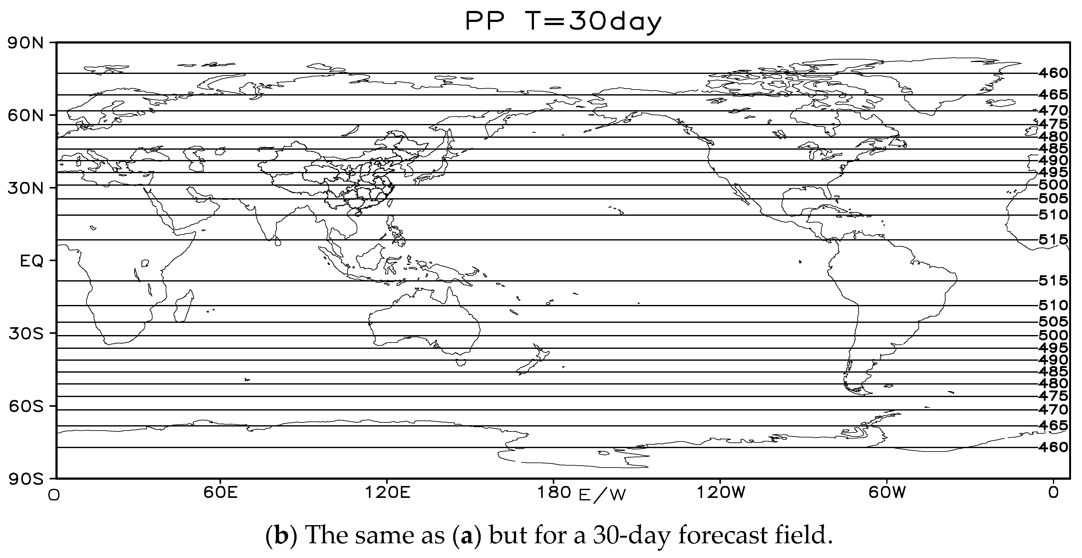
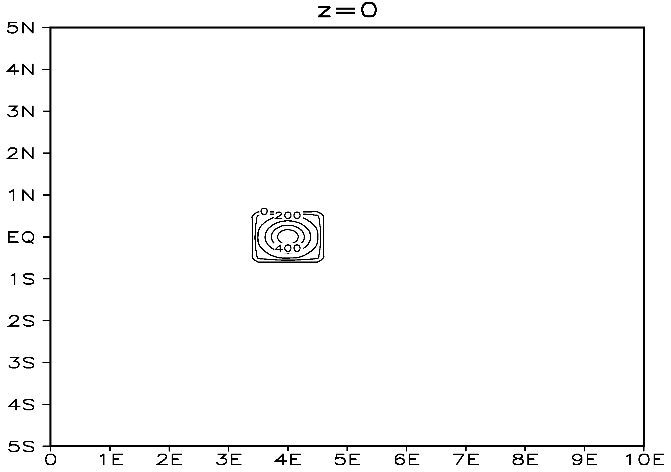
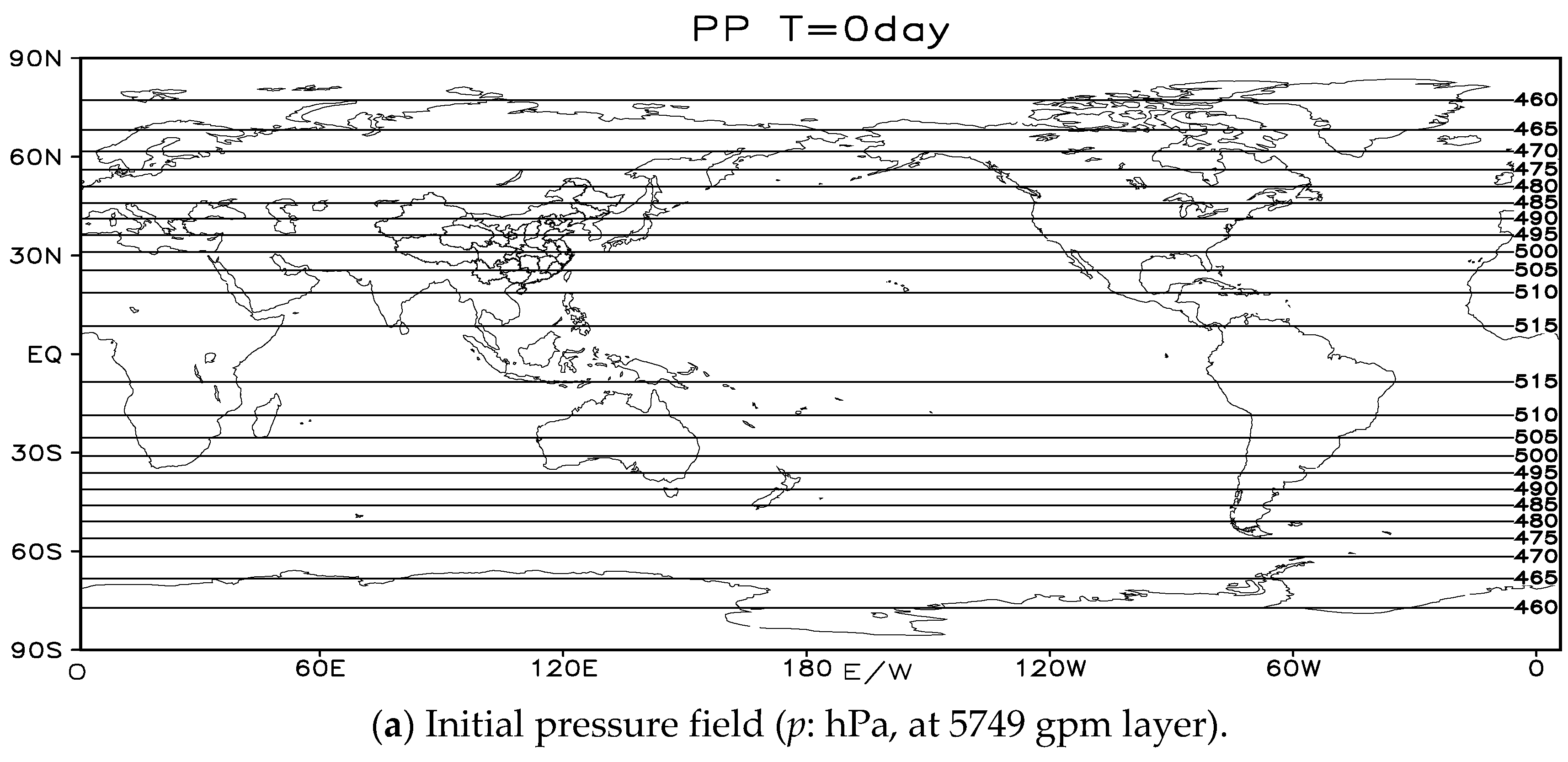
After substituting the above p, T, q, u, v, and w initial value fields into the atmospheric motion equation, it is not difficult to find a frictionless, water vapor-free process: $\frac{dp}{dt}=\frac{dT}{dt}=\frac{du}{dt}=\frac{dv}{dt}=\frac{dw}{dt}\equiv 0$, so the equilibrium flow test is the “eternal” motion of the model atmosphere in horizontal constant angular velocity. In the initial value field, the p, T, and u fields are east–west parallel “straight lines” in any height layer (Figure 1a for the p field); because the path on the “straight line” flow field overlaps with the trajectory, the time integral p, T, and u fields should remain unchanged.

The quasi-geostrophic equilibrium flow test results are as follows: on the A–B-grid mapping a global 1° × 1° mesh, from the pressure, temperature, and wind initial value fields to the 30 d integration fields, with time steps of 600 s, they hardly change (Figure 1b for the p field) on any contour plane. The fact that atmospheric mass, energy, and momentum fields flow in parallel and uniformly, and the “cubic” advection is compatible with linear advection, shows that the nonlinear bicubic surface fitting of the linear pressure/mass), temperature/energy, and wind/momentum fields can ensure that the horizontal path of the upstream point coincides with its trajectory.

6.3. Cross-Polar Flow Test

We design an ideal horizontal, two-dimensional cross-polar flow test to examine the viability and accuracy of the upstream point in the spline format on the A–B-grid, including the polar regions and the poles, to test the correctness of the procedure of the horizontal motion equation at the North Pole and the South Pole, and to address the issues of the overly dense grid in the polar region and the singularity of the poles.

Suppose the advection satisfies the geostrophic equilibrium and the initial perturbation pressure field is taken as follows:

$$p=p_0\exp (-\frac{2\mathsf{\Omega }{r}_e{v}_0}{\mathrm{R}{T}_0}{\sin }^3\mathsf{\phi }\cos \mathsf{\phi }\sin \lambda )$$

(63)

Suppose in the above equation that $p_0=1000$ hPa, $T_0=300$ K, and $v_0=20$ ms⁻¹.

Then, the spline-format horizontal geostrophic wind $(u_{\mathrm{g}},v_{\mathrm{g}})$ is

$$\begin{gathered} (u_{\mathrm{g}},v_{\mathrm{g}})=\frac{\mathrm{R}{T}_0}{f}[-{(\ln p)}^y,{(\ln p)}^x] (-\frac{\pi }{2}\le \mathsf{\phi }<0, 0<\mathsf{\phi }\le \frac{\pi }{2}) \\ {u}_{\mathrm{g}}=v_{\mathrm{g}}=0 (\mathsf{\phi }=0) \end{gathered}$$

(64)

and the initial value of the horizontal geostrophic wind is obtained as

$$u_{\mathrm{g}}=v_0(3{\cos }^2\mathsf{\phi }-{\sin }^2\mathsf{\phi })\sin \mathsf{\phi }\sin \lambda , v_{\mathrm{g}}=-v_0{\sin }^2\mathsf{\phi }\cos \lambda$$

(65)

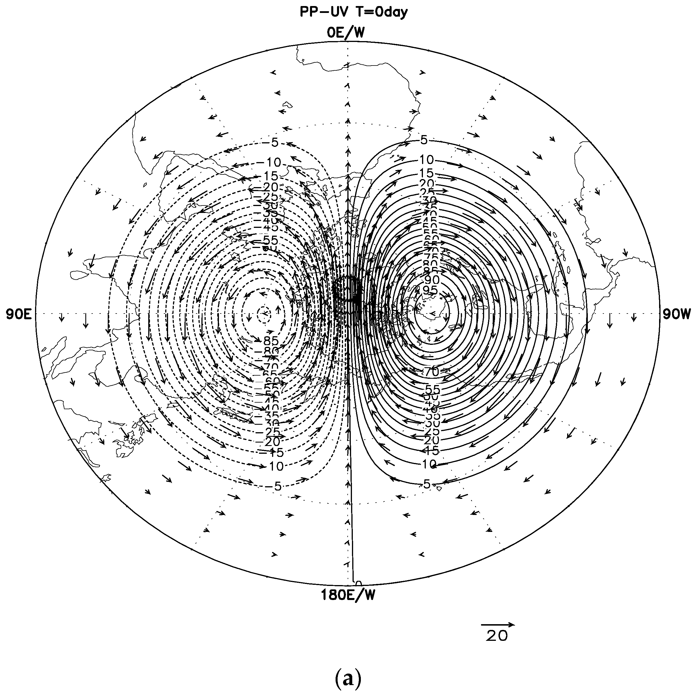
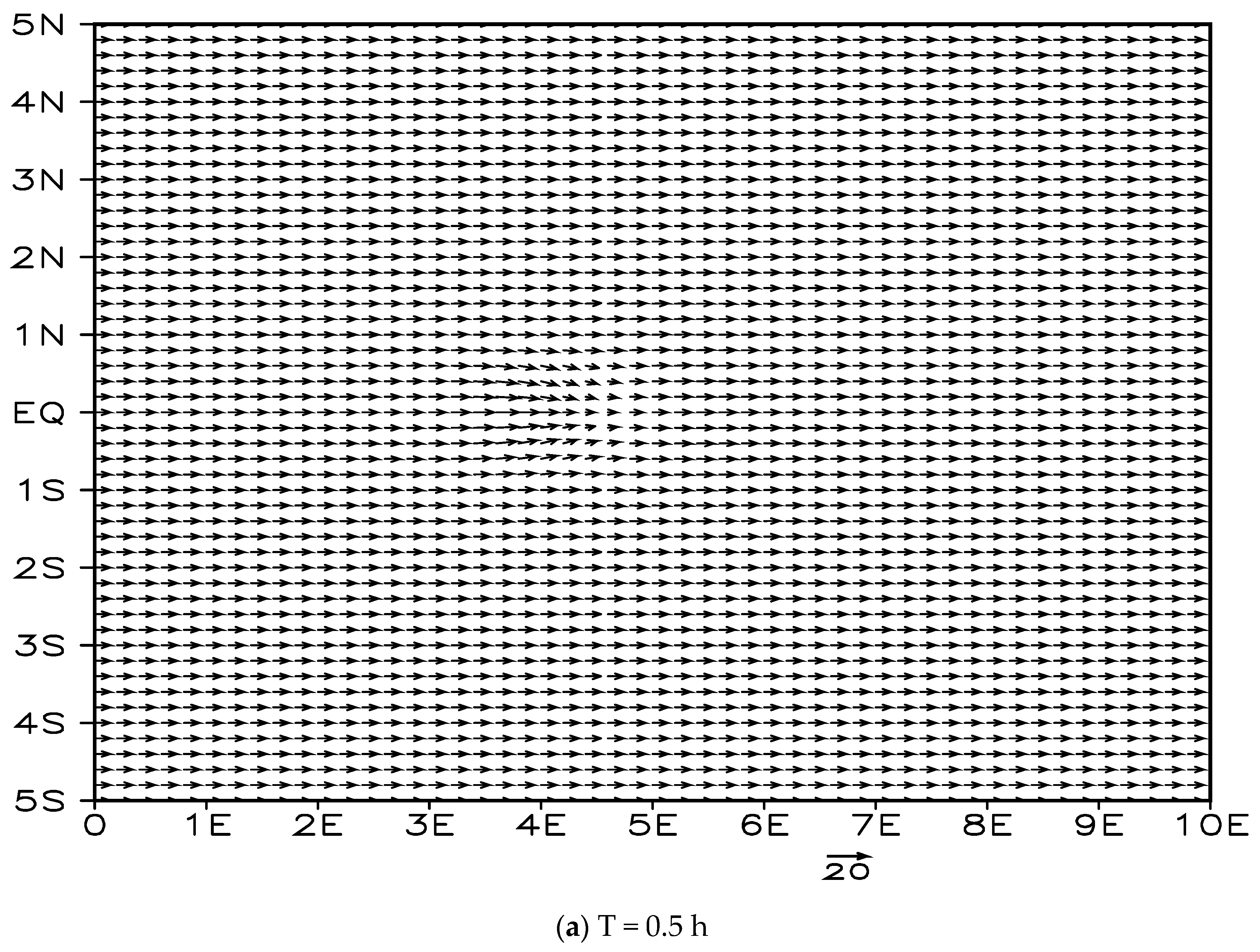
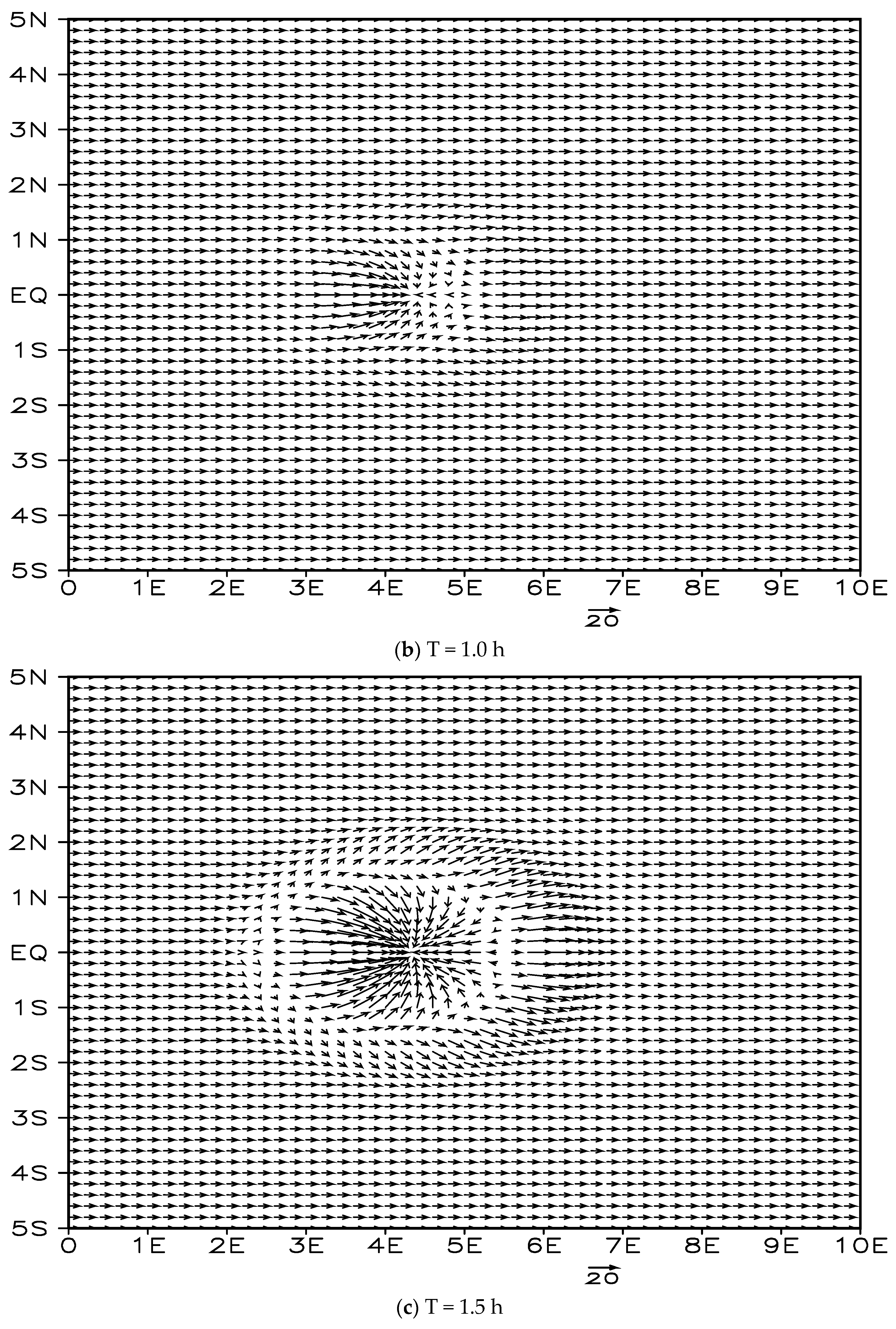
The cross-polar flow is characterized by (Figure 2): ${(u_{\mathrm{g}})}_N=0$, ${(v_{\mathrm{g}})}_N=-v_0$ at the North Pole; ${(u_{\mathrm{g}})}_S=0$, ${(v_{\mathrm{g}})}_S=-v_0$ at the South Pole, which is consistent with the definition of horizontal wind at the pole; and $u_{\mathrm{g}}=v_{\mathrm{g}}\equiv 0$ at the equator.

From Equation (6), it is found that the exact solution of the geostrophic wind keeps parallel/perpendicular to the perturbed pressure field contour/gradient, and the path of the upstream point obtained by the flow line should coincide with the trajectory, without change of the mass field.

The log-pressure ($\ln p$) field of each layer is fitted to a spherical bicubic surface, allowing for a diagnosis of the horizontal geostrophic wind (Figure 2a).

Cross-polar flow tests with a horizontal resolution of 1° × 1° are designed (

Table 2. Cross-polar flow tests.

Cross-Polar Flow Tests	Geostrophic Wind	Time Step	Integration Time
Test 1	$(u_g,v_g)$	300 s	10 d
Test 2	$(u_g+5\cos \mathsf{\phi },v_g)$	300 s	10 d

):

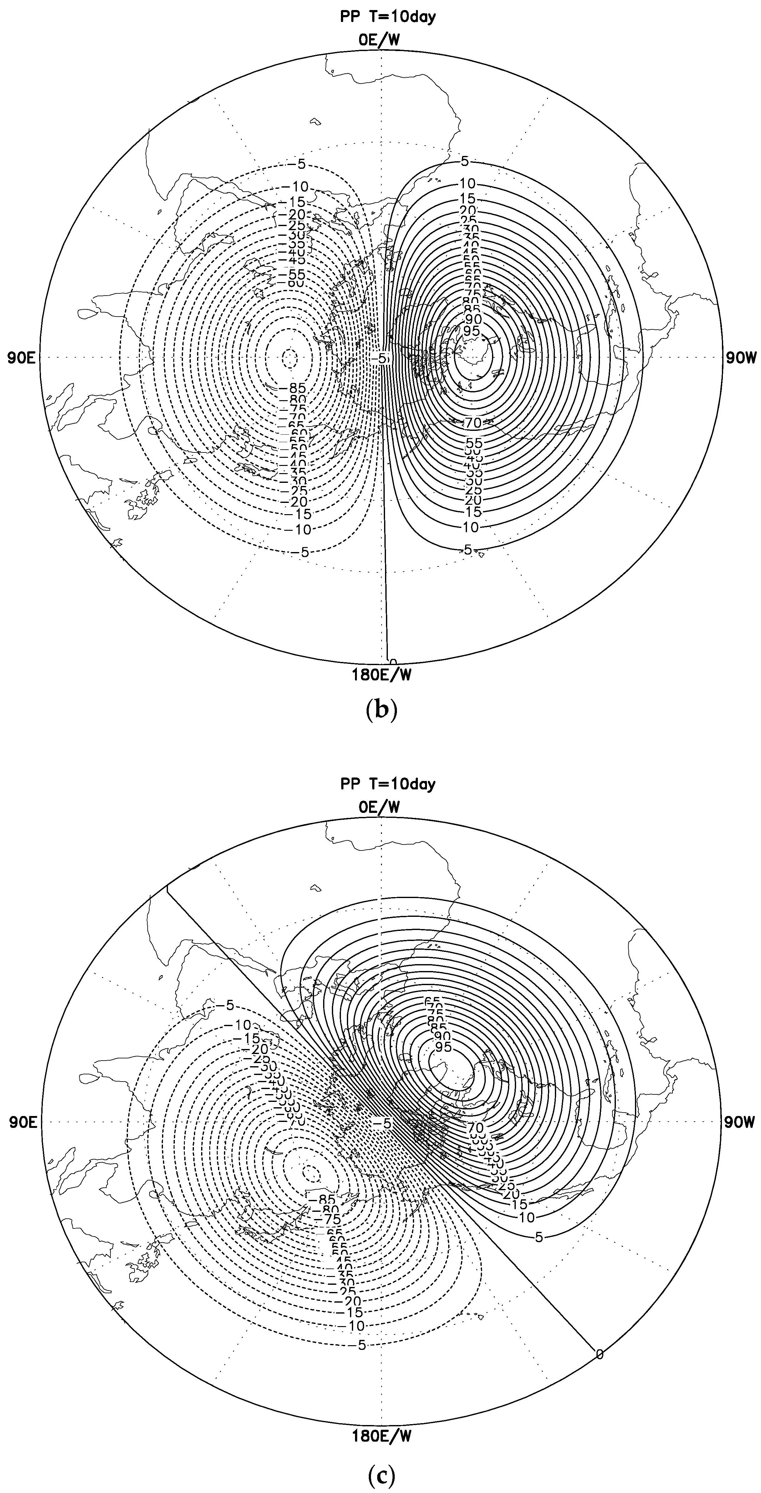
The perturbation pressure/mass field should not change over time, and the geostrophic wind in Test 1 should maintain its parallel alignment with the isobars; however, in Test 2, with a constant angular velocity applied ($5\cos \mathsf{\phi }$ ms⁻¹), plus the effect of advection, the perturbation pressure/mass field can only rotate uniformly.

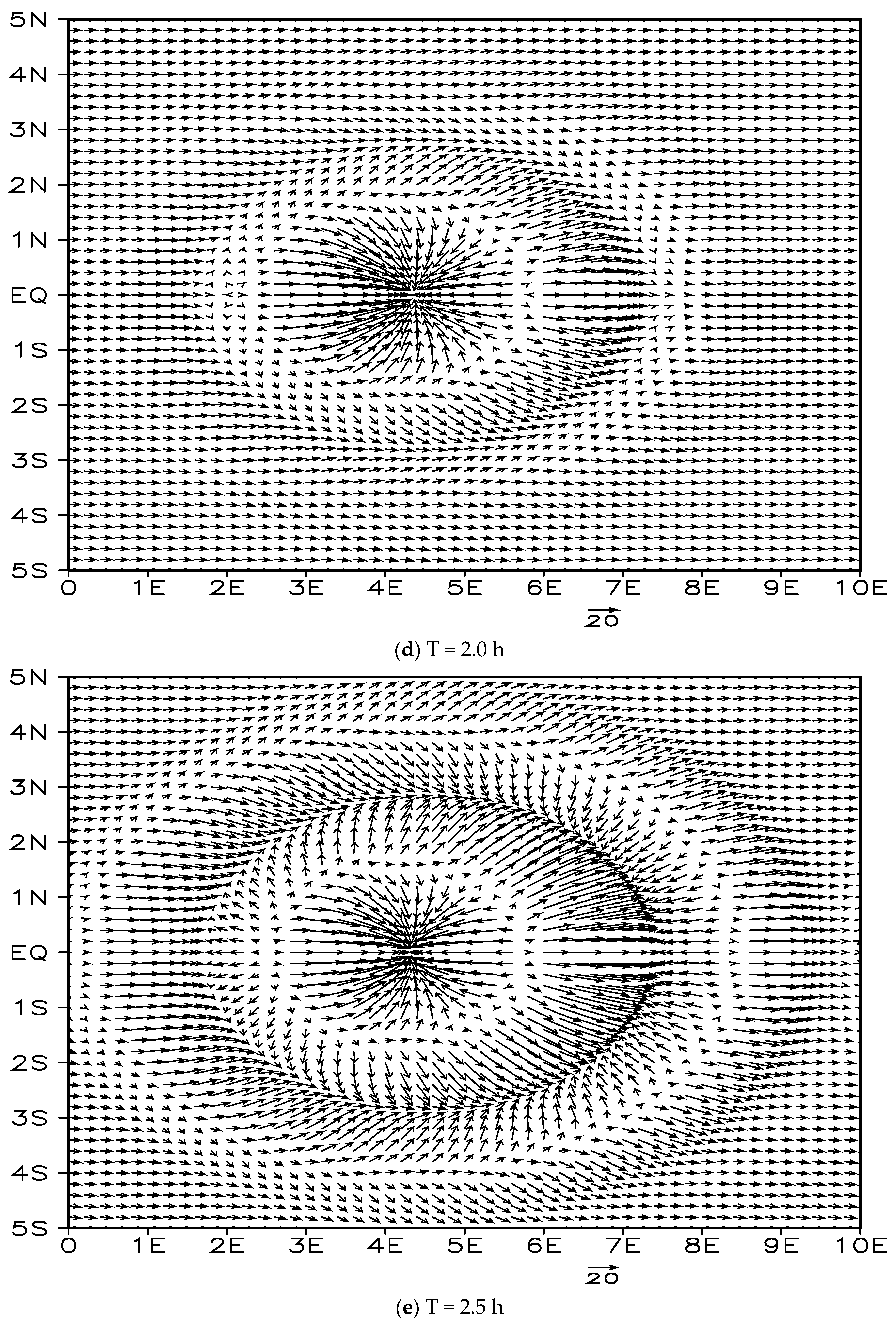
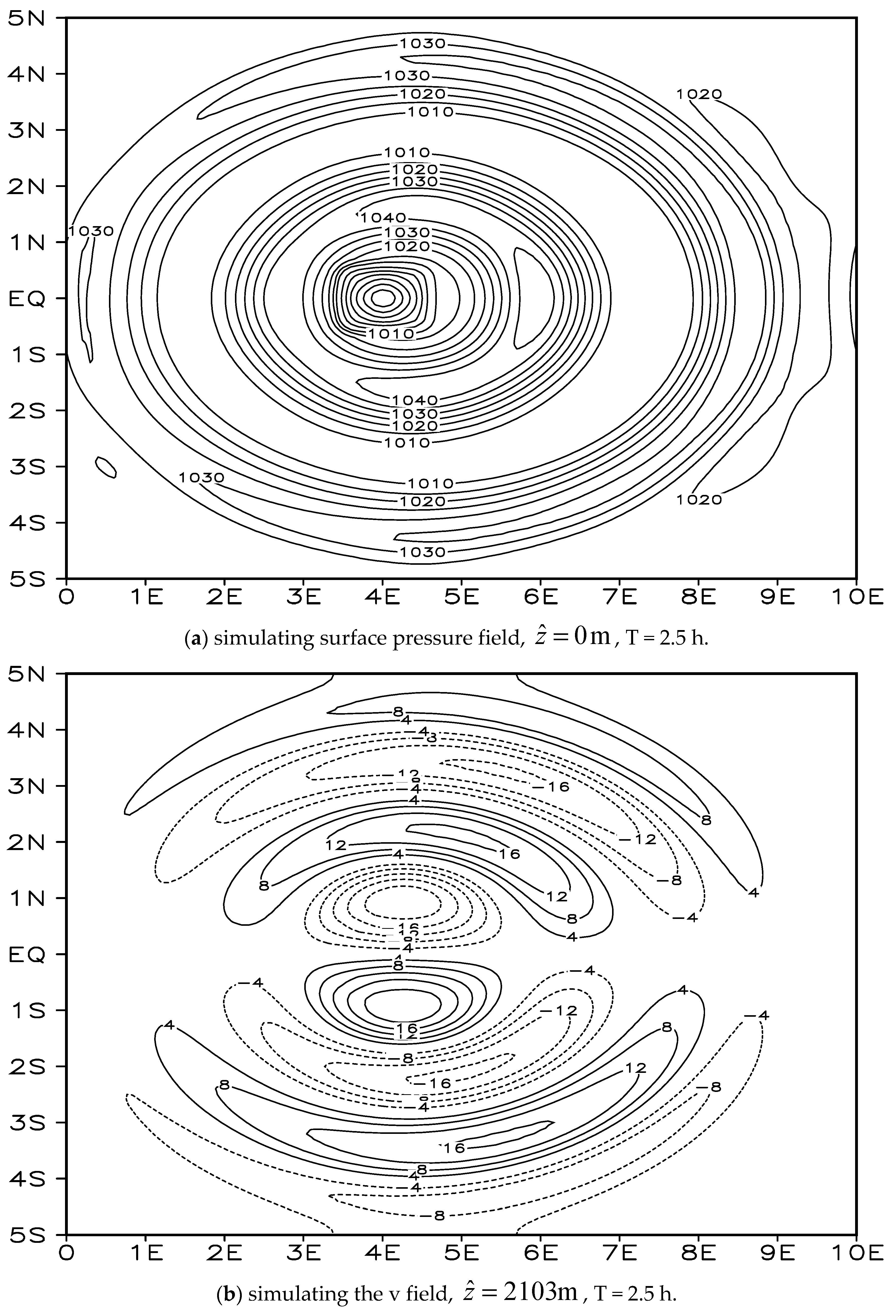
The results of the cross-polar flow test are as follows (see Figure 2 for the Northern Hemisphere): compared with the initial value field (Figure 2a), the wind and pressure fields in Test 1 hardly change with time (Figure 2b); in Test 2, after being integrated for 10d (Figure 2c), the geostrophic wind and pressure field relationship is maintained globally, including polar regions, the perturbation pressure/mass field has little deformation, and there is little mass change despite wind and pressure field rotation.

6.4. Rossby–Haurwitzwave Test

The Rossby–Haurwitz wave, often known as the “R–H wave”, is an approximate solution to the linear barotropic vorticity equation that, given certain assumptions, becomes an exact solution.

If the Coriolis force ($f=2\mathsf{\Omega }\sin \mathsf{\phi }$) changes slowly and only describes the R–H wave in the Northern Hemisphere, then f is set at 45° N and taken as $f=f_0=2\mathsf{\Omega }\sin (\frac{\pi }{4})$. Next, let the perturbed geopotential height field h of the R–H wave (the exact solution) be as follows:

$$h(\lambda ,\mathsf{\phi },z)=2\mathsf{\Omega }\sin (\frac{\pi }{4})\frac{\mathsf{\Psi }(\lambda ,\mathsf{\phi },z)}{g}$$

(66)

where $\mathsf{\Psi }$ is a stream function, which has a wind–pressure field relationship with the divergence-free wind $(u_{\mathsf{\Psi }},v_{\mathsf{\Psi }})$

$$(u_{\mathsf{\Psi }},v_{\mathsf{\Psi }})=(-\frac{{\mathsf{\Psi }}^{\mathsf{\phi }}}{r_e},\frac{{\mathsf{\Psi }}^{\lambda }}{r_e\cos \mathsf{\phi }})$$

(67)

According to the aforementioned Equation (9), the path of the upstream point generated by the flow line will coincide with the trajectory, without changing the mass field. Similarly, the divergence-free wind stays exactly parallel/perpendicular to the stream function field contour/gradient.

Suppose that $h_0$ ($h_0=300$ gpm) is the disturbance amplitude, we take $u_0=20$ m/s, we let $\mathrm{C}=\frac{g{h}_0}{r_e{f}_0}$, and we set the “4-latitudinal wave” stream function field $\mathsf{\Psi }$ as

$$\mathsf{\Psi }=\mathrm{C}{\cos }^2\mathsf{\phi }\cos (4\lambda )+r_e{u}_0(1-\sin \mathsf{\phi })\widehat{=}\mathsf{\Psi }1+\mathsf{\Psi }2$$

(68)

By substituting Equation (68) into Equation (67), we obtain the following:

$$\begin{array}{c}{u}_{\mathsf{\Psi }}=u_{\mathsf{\Psi }1}+u_{\mathsf{\Psi }2}: u_{\mathsf{\Psi }1}=\mathrm{C}\sin (2\mathsf{\phi })\cos (4\lambda ), u_{\mathsf{\Psi }2}=u_0\cos \mathsf{\phi }\\ v_{\mathsf{\Psi }}=-4\mathrm{C}\cos \mathsf{\phi }\sin (4\lambda )\end{array}$$

(69)

where $u_{\mathsf{\Psi }2}$ is the latitudinal constant angular velocity.

$\mathsf{\Psi }$ is fitted to a spherical bicubic surface before each time step integration to obtain its slope ${\mathsf{\Psi }}^x$ and ${\mathsf{\Psi }}^y$, and then we have a wind–pressure field relationship in “spline format” (compare with Equation (67)):

$$(u_{\mathsf{\Psi }},v_{\mathsf{\Psi }})=(-{\mathsf{\Psi }}^y,{\mathsf{\Psi }}^x)$$

(70)

Here, only two-dimensional, ground-level R–H wave advection tests are performed.

First, the height amplitude $h_0$ is converted to “isothermal atmospheric” pressure amplitude $p_0$, that is, the geopotential height perturbation field is converted to a pressure perturbation field, and then we have the following (let $p_N=840$ hPa, $T_N=273.15$ K, $p_N$ and $T_N$ be the ground North Pole pressure and temperature, and $T_N$ be the isothermal atmospheric temperature):

$$p_0=p_N[1-\exp (-\frac{g{h}_0}{\mathrm{R}{T}_N})]$$

(71)

Here, four R–H wave tests are designed (

Table 3. Rossby–Haurwitz wave tests.

Rossby-Haurwitz Wave	Divergence-Free Wind Field	Time Step	Time Integral
Test 1	$(u_{\mathsf{\Psi }1}+20\cos \mathsf{\phi },v_{\mathsf{\Psi }})$ m/s	600 s	100 d
Test 2	$(u_{\mathsf{\Psi }1}+30\cos \mathsf{\phi },v_{\mathsf{\Psi }})$ m/s	600 s	100 d
Test 3	$(u_{\mathsf{\Psi }1}+30\cos \mathsf{\phi },v_{\mathsf{\Psi }})$ m/s	600 s	300 d
Test 4	$(u_{\mathsf{\Psi }1}+30\cos \mathsf{\phi },v_{\mathsf{\Psi }})$ m/s	60 s	300 d

).

For the results of the R–H wave test, see Figure 3 for the Northern Hemisphere and specifically Figure 3a for the initial value field.

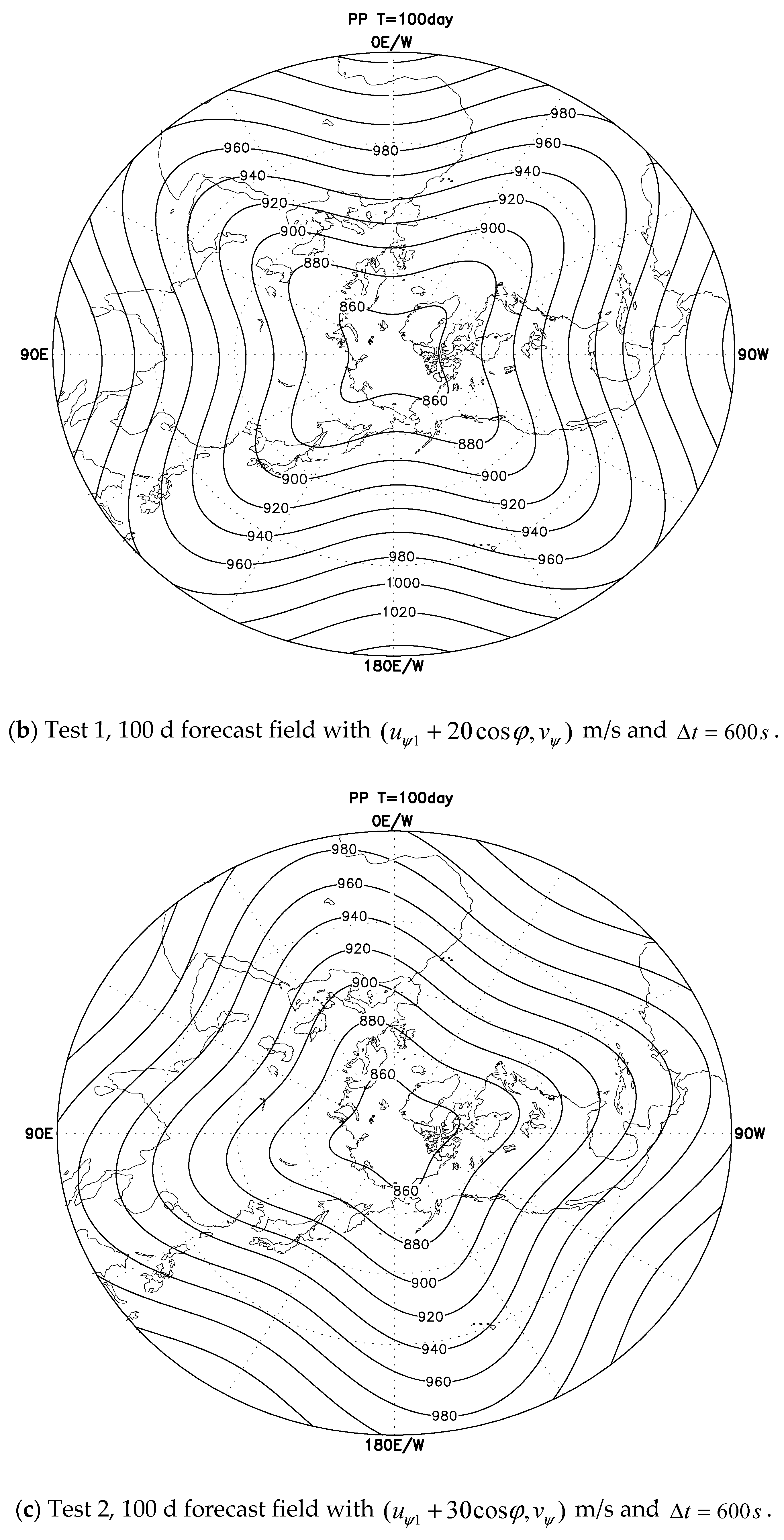
Test 1 flow field has a constant equal latitudinal angular velocity $u_{\mathsf{\Psi }2}=20\cos \mathsf{\phi }$ (m/s). The path of the upstream point remains parallel to the trajectory, the forecast flow function or mass field does not rotate, bicubic surface fitting can preserve the spherical symmetry of the original flow field, and a 100 d integrated perturbed pressure/mass field has insignificant deformation and error. Additionally, the divergence-free wind–pressure field relationship is maintained (Figure 3b).

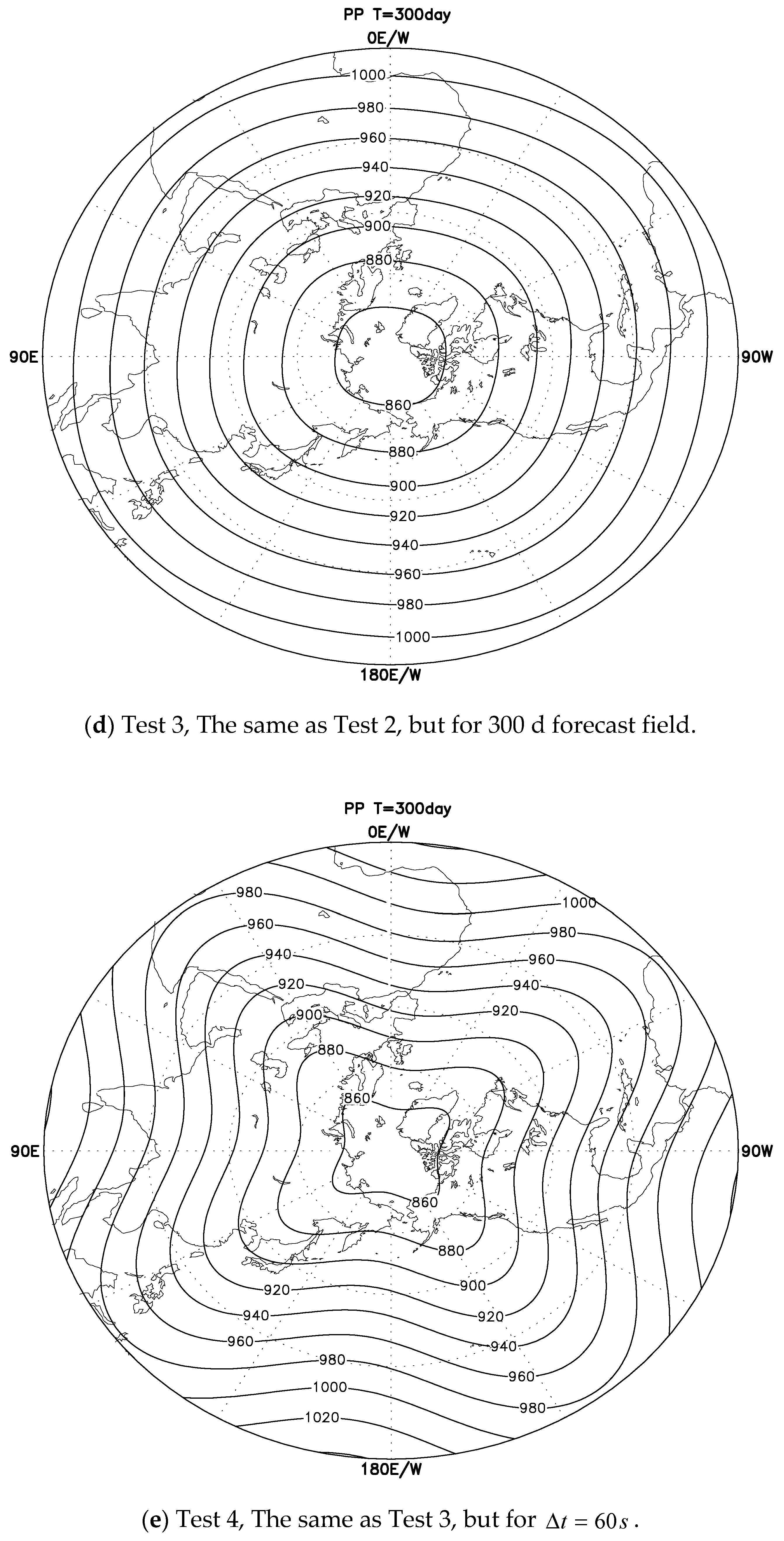
Tests 2–4 all add another $10\cos \mathsf{\phi }$ (m/s) of equal latitudinal angular velocity; they turn as $u_{\mathsf{\Psi }2}=30\cos \mathsf{\phi }$ (m/s) (Table 3). In Test 2, under the action of advection at $(u_{\mathsf{\Psi }1}+30\cos \mathsf{\phi },v_{\mathsf{\Psi }})$ m/s, the pressure/mass field rotates due to the addition of the zonal angular velocity, and the deformation of the 100 d integrated “rotating” mass field (Figure 3c) is a lot larger than that in Test 1 (Figure 3b), and when the integration is extended to 300 d in Test 3, the pressure field has closely become “round” (Figure 3d). The 300 d predicted air pressure field in Test 4 (Figure 3e) has much more “fidelity” than that in Test 3 (Figure 3d), but with a time step of 60 s, that is, 10-times higher time precision while the computation volume also grows by 10 times.

The R–H wave test proves that when using spline forecast, the amplitude error of the wave, which can mean the pressure field becomes “round”, is monotonically bound, correct fluctuation phase propagation, which means that phase propagation is independent of spatial resolution, is maintained, and there is a convergence between fidelity and time resolution.

7. Density Flow Test

7.1. Initial Value Field

The divergence field comprises acoustic wave propagation, and the density flow test calculates the non-hydrostatic fully compressible air parcel displacement, divergence, and pressure and temperature field fluctuation.

The density flow test is a two-dimensional $(x,z)$ ideal field test where the initial value field is still taken as a 3D model atmosphere, but only the middle vertical cross-section grid points in the y-direction are used for the time integration. Each time step is given the same forecast values for the other grid points in the y-direction, and then it is set to $P^y=P^{xy}\equiv 0$. The typical density flow test has a spatial resolution of $\Delta x=\Delta z=100$ m without topography; in $(x,y,z)$, the area is taken as (0:512, −4:4, 0:53), and then it always is set to $P(x,y,z)\equiv P(x,0,z)$.

The x-direction is a periodic cubic spline, which means that there are no boundaries; the y-direction is the rigid boundary $P^y\equiv 0$, and the z-direction comprises the top and bottom layer, where the air pressure and the perturbation pressure from the hydrostatic equilibrium boundary make the top and bottom layer $w=a_w\equiv 0$. While temperature, wind, and displacement are all forward and backward difference boundaries, which lead the divergence to act on and change the surface pressure and temperature field on the bottom layer, causing the surface pressure to become completely elastic, meanwhile, the top layer air pressure, temperature, and wind all remain constant.

The undisturbed initial value field is the dry hydrostatic atmosphere, $q=u=v=w=0$, the ground pressure is 1000 hPa, and the model atmospheric initial potential temperature ($\theta$) field is 300 K, meaning the ground-layer temperature is 300 K.

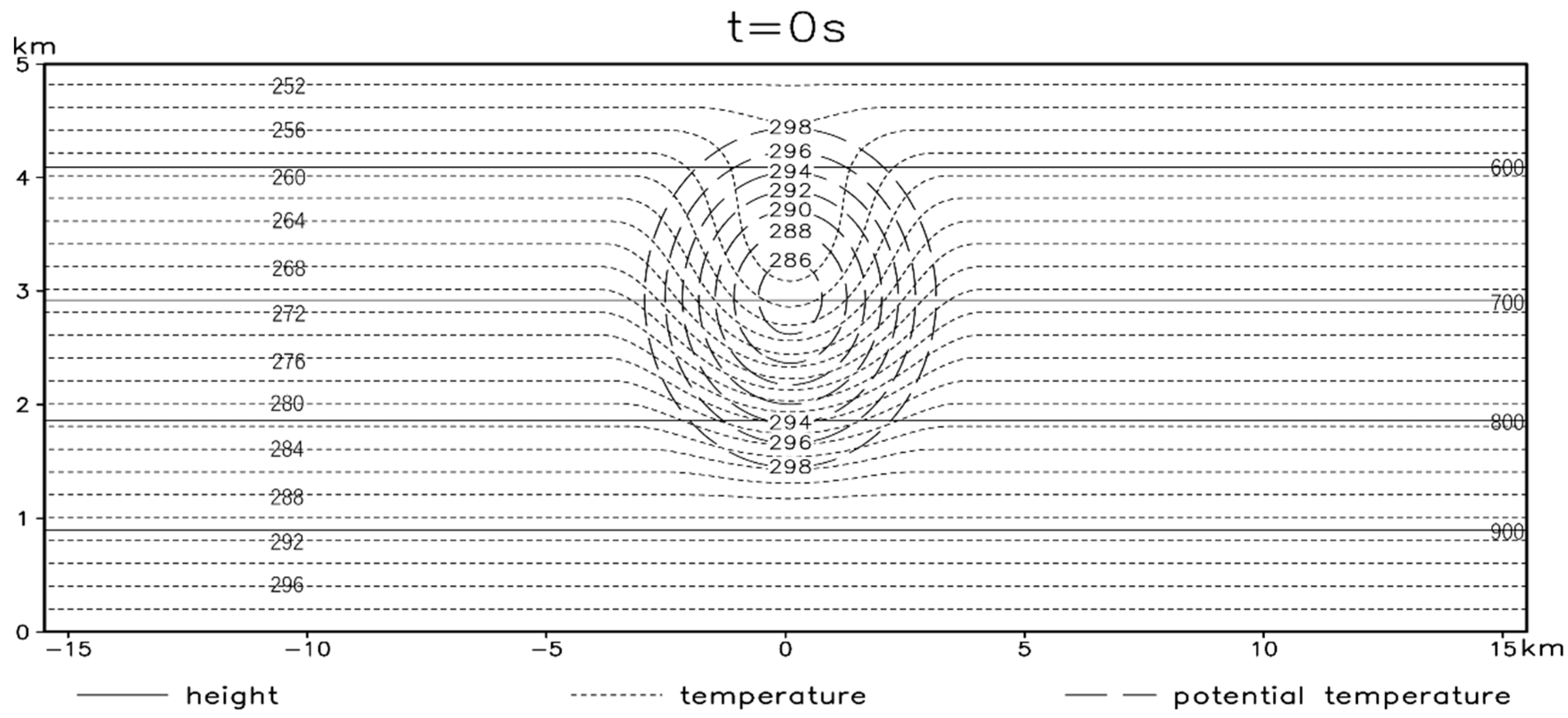
A circular, cross-sectional cold surge is placed in the center of the undisturbed initial value field (Figure 4), that is, we set the following:

$$\begin{array}{c}\Delta \theta =\frac{-15}{2}[\cos (\pi \cdot \mathrm{L})+1],\\ \mathrm{L}=\sqrt{{\left(\frac{x_{\mathrm{i}}-x_{\mathrm{c}}}{{\mathrm{r}}_x}\right)}^2+{\left(\frac{z_{\mathrm{k}}-z_{\mathrm{c}}}{{\mathrm{r}}_z}\right)}^2}\le 1, \mathrm{i}=0,1, \dots , 512; \mathrm{k}=0,1, \dots , 53\end{array}$$

(72)

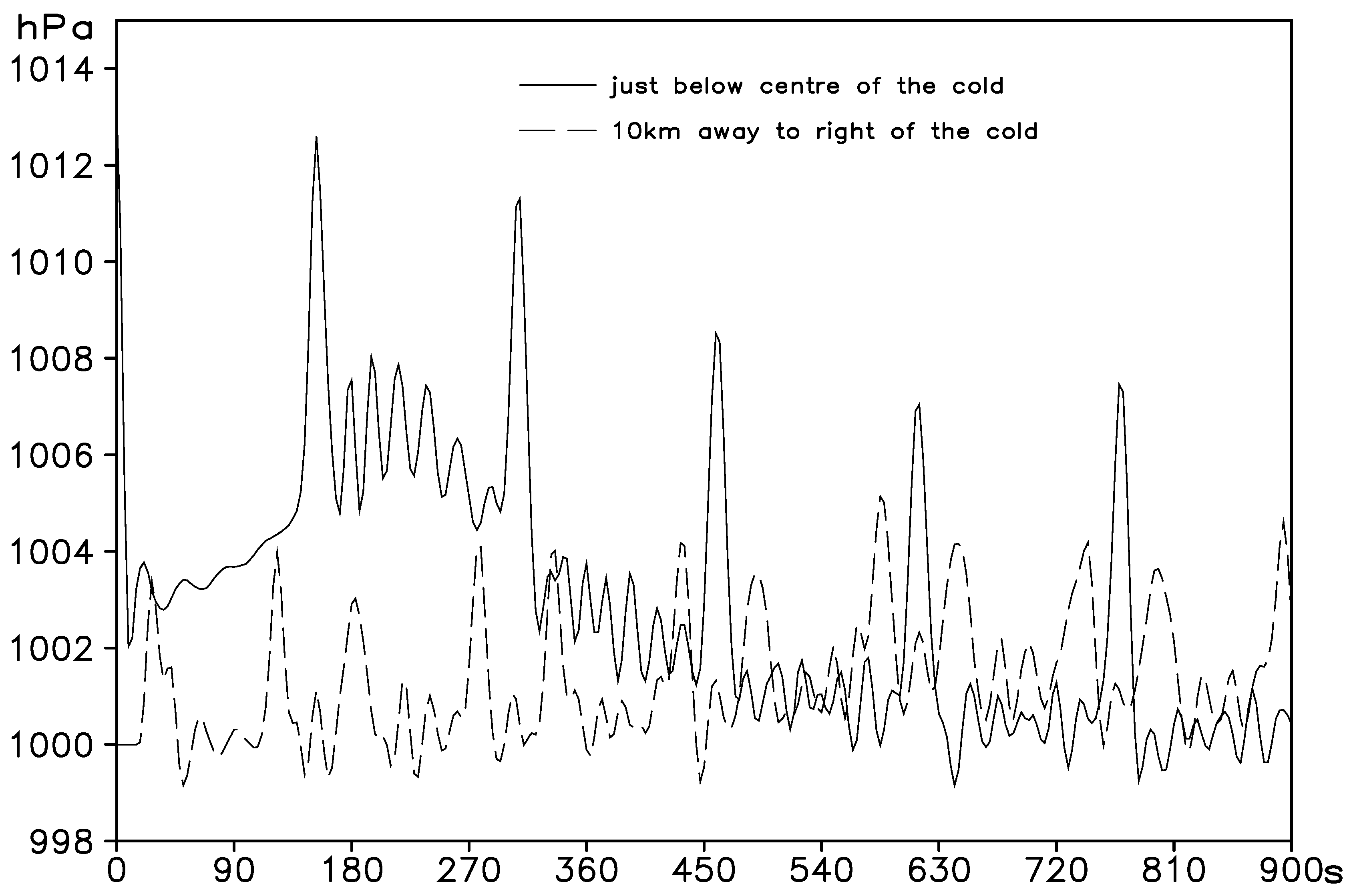
Here (Figure 4), take $(x_{\mathrm{c}},z_{\mathrm{c}})=(256\times 100 \mathrm{m}, 30\times 100 \mathrm{m})$ as the cold surge center point, and $({\mathrm{r}}_x,{\mathrm{r}}_z)=(40\times 100 \mathrm{m}, 20\times 100 \mathrm{m})$ as the cold surge $(x,z)$ direction radius. In the cold surge center point: $\mathrm{L}=0$ and $\Delta \theta$ = −15 K. By using the hydrostatic force equation and the potential temperature conservation Poisson equation, the perturbation initial value field pressure and temperature distribution are obtained. Because of the cold surge, the initial value of the air pressure field changes a little; for example, the ground pressure directly below the cold surge center reaches 1013.21 hPa.

By using the separation hydrostatic pressure method, the “time-varying reference atmosphere” and vertical acceleration $a_w$ are calculated at each time step, and then the initial value field $a_w$ is a non-null distribution only in the cold surge.

7.2. Temporal Resolution and Spatial Smoothing

The density flow test benchmark reference solution takes a time step of 0.1 s, with a time integration of 900 s.

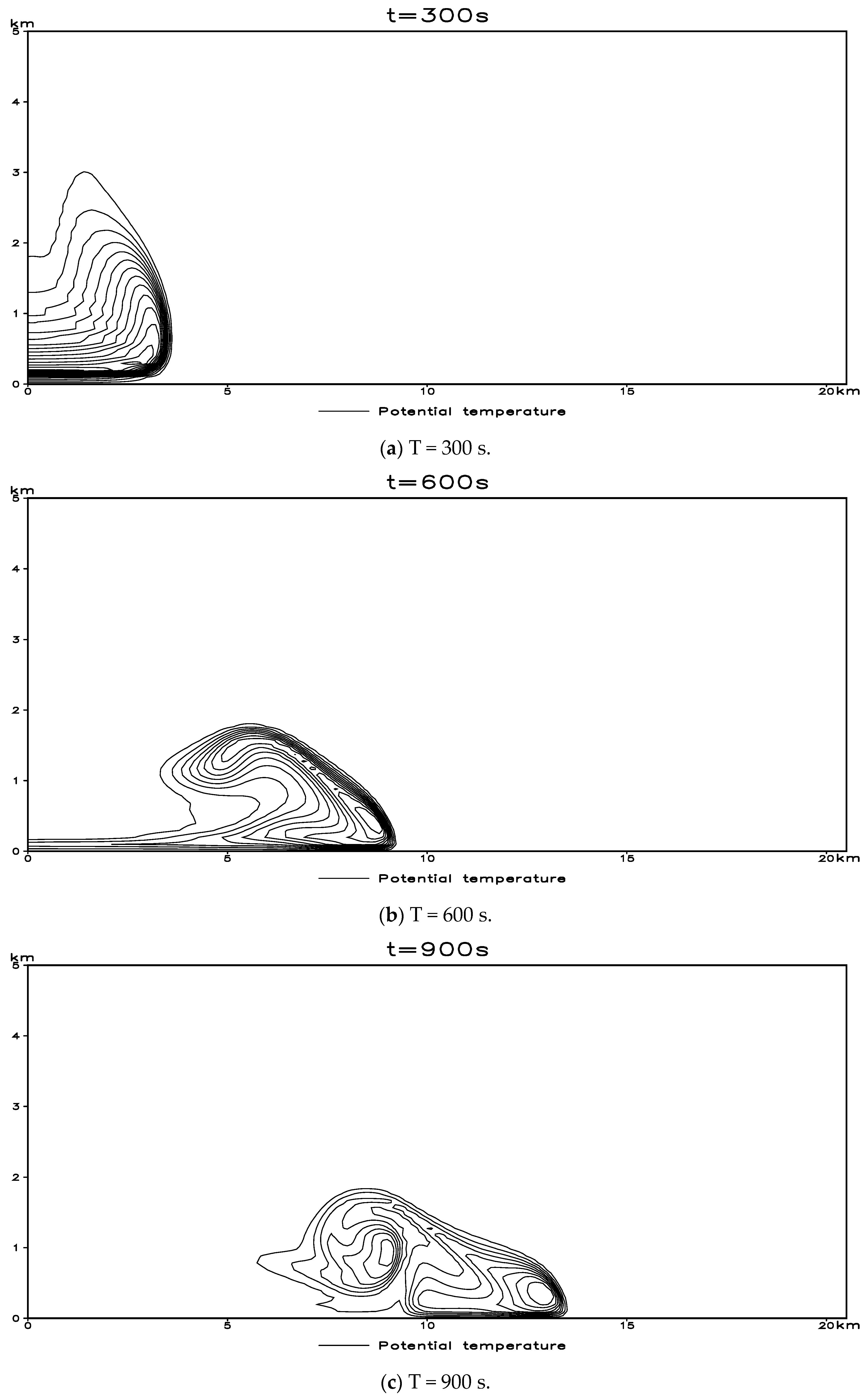
In density flow test 1 (Figure 5), with a time step of 0.1 s, three-point spatial smoothing with a vertical wind field coefficient of 1/3 and three-point smoothing with a horizontal pressure field coefficient of 1/2 are performed every three time steps (0.3 s). In the smoothing of the barometric field, the corresponding Poisson equation “adiabatic temperature change” smoothing, is performed on the temperature field (called “potential temperature conservation”-pressure temperature field smoothing).

Density flow test 2 is similar to test 1 but with a 0.125 s time step (Figure 6). Vertical wind field smoothing, pressure, and temperature field “potential temperature conservation” smoothing, and three-point smoothing with divergence field horizontal and vertical coefficients of 1/2 are also carried out at every time step (0.125 s), respectively, to prevent the growth and propagation of the acoustic waves.

Density flow test 1 and 2 both extend the integration to 1200 s, and the results of these tests are roughly similar (Figure 5 and Figure 6).

In addition to the benchmark reference solution being in a higher-order-precision spline format (its linear principal part is the second-order central difference), they also have different boundary conditions and spatial smoothing schemes. Straka et al. (1993) proposed the density flow test benchmark reference solution in linear format with various resolutions.

7.3. Density Flow Test Analysis

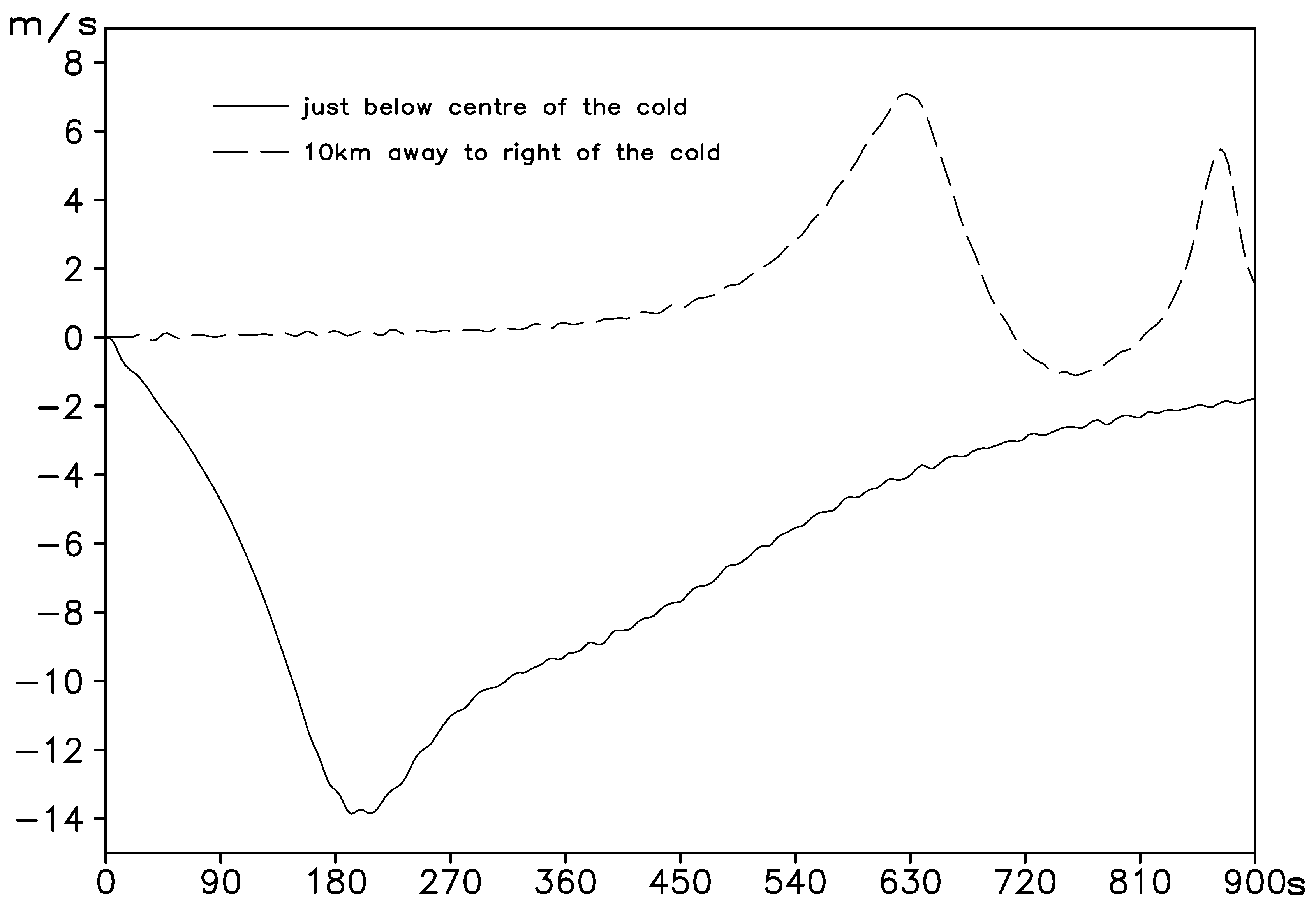
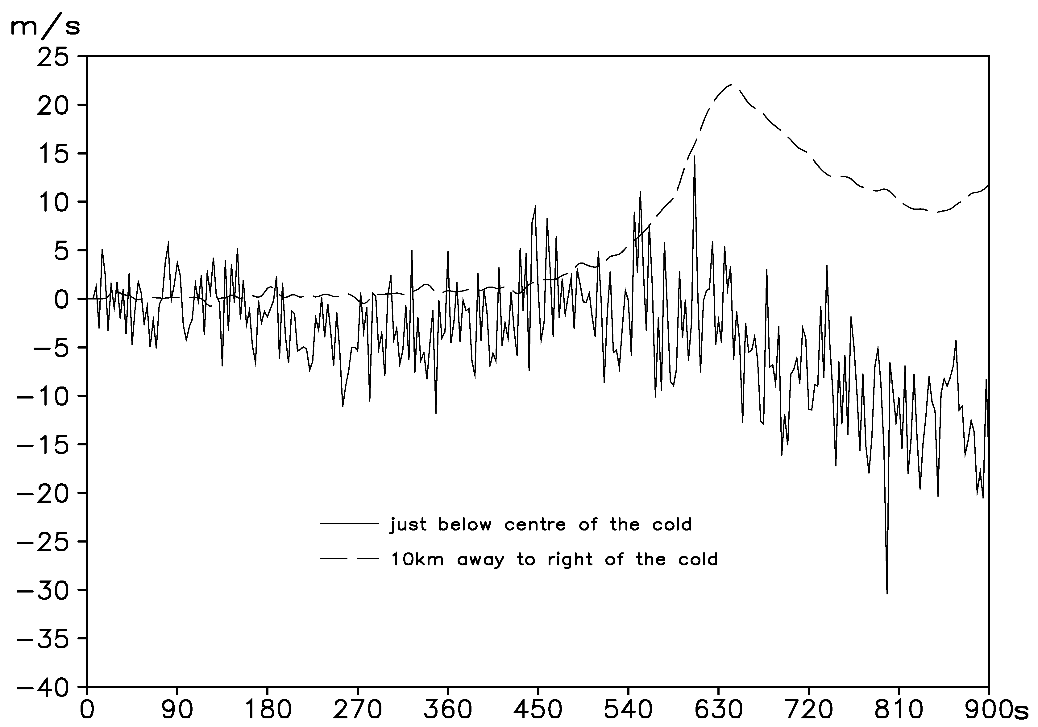
A highly nonlinear density flow test reveals the whole “cold surge sinking → bottom cold air accumulation → Kelvin-Helmholtz horizontal wind shear formation at cold front → unstable vortex formation” evolution process, which is an “acoustic + gravity wave” propagation process.

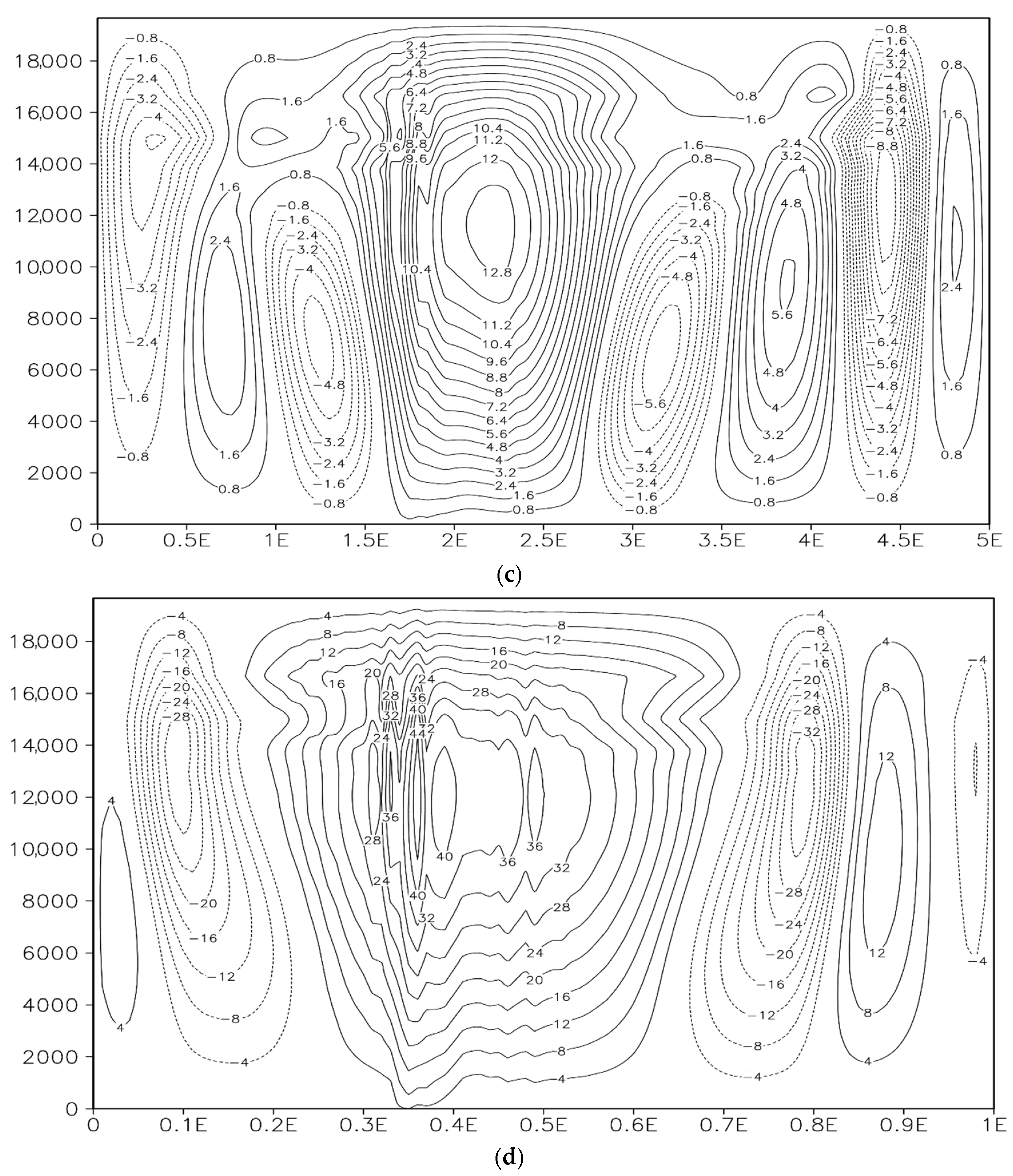
For this density flow test (Figure 5 and Figure 6), under negative buoyancy of the vertical pressure gradient force, the cold surge accelerates sinking, and it accumulates after hitting the bottom, forming a sinking divergence “cold front” air flow. The cold air is divided into two (for a 3D test, cold air will be in circular fluctuation) symmetric cold fronts on the left and right (Figure 5 and Figure 6 only show a forward movement along x).

The results of the density flow test show that after 300 s of integration, the cold surge’s main body reaches the bottom, forming strong horizontal wind vertical shear in front of the cold front, achieving Kelvin–Helmholtz shear instability. This forms the first front vortex (Figure 5a and Figure 6a); after 600 s of integration, the first vortex rapidly intensifies, with a “multi-vortex” rolling on the back, while the front forms a second vortex (Figure 5b and Figure 6b); once integrated for 900 s, the first vortex has developed into a circular vortex, and the second vortex is still developing, followed by the development of a third vortex (Figure 5c and Figure 6c); and once integrated for 1200 s, the cold front continues to move forward, with a three-vortex pattern maintained roughly (Figure 5d and Figure 6d).

As can be seen in Figure 7 and Figure 8, before the cold surge reaches the bottom, the ground pressure directly below the cold surge center drops rapidly, down to about 1002 hPa. During this process, the near-ground layer (up to 900 m) keeps a sinking motion, with the vertical wind speed reaching about −14 ms⁻¹ when being integrated for 200 s. The cold surge process is divided into forward compression and rebound (the so-called “fully compressible” = “fully elastic”). When the cold surge hits the bottom for the first time, the surface pressure once again increases to 1013 hPa, and then the first rebound occurs, and the pressure returns to about 1005 hPa, with a big shock wave amplitude of about 7–8 hPa and a shock process lasting for about 30 s, followed by a number of small “fully elastic” waves with an amplitude of about 3 hPa. The big shock wave is a gravity wave, with an interval of about 150 s, and it weakens toward an “undisturbed surface pressure of 1000 hPa”. Similar to the surface pressure changes directly below the cold surge center, the surface pressure 10 km right of the cold surge also presents shock wave evolution, with wave amplitudes from about 4 hPa to about 1 hPa, and an interval of about 75 s; that is, the latter has the smaller amplitude but the higher frequency, which shows the gravity wave’s horizontal propagation and divergence characteristics. At the same time, the maximum vertical wind at 900 m above 10 km in front of the cold surge is 7.5 ms⁻¹ when a cold front passes; then, the rising wind speed is rapidly reduced, falling to −1 ms⁻¹ sinking motion once, and then returns to 5.5 ms⁻¹ rising motion when the secondary cold front passes.

As shown in Figure 9, the surface horizontal wind directly below the cold surge presents acoustic vibration, with an acoustic amplitude of about 0.002 ms⁻¹, and the surface horizontal wind 10 km ahead of the cold surge shows gravity wave characteristics; corresponding to the addition of the aforementioned vertical wind, the horizontal wind speed gradually increases before the passage of the cold front, reaching a maximum speed of 23 ms⁻¹ when the front passes after being integrated for 600 s. It is clear that the evolution of horizontal wind includes the propagation of acoustic and gravity waves, with the gravity “fast” wave having a 1 ms⁻¹ periodic oscillation amplitude superimposed.

8. Gravity Wave Test

A 3D gravity wave test is performed to test the topographic-perturbation-caused gravity wave process of the hydrostatic/non-hydrostatic dynamic core, producing comparable results.

8.1. Initial Value Field

The initial value field of the gravity wave test is an equilibrium flow that satisfies the hydrostatic equilibrium and proves to be a horizontal-motion quasi-geostrophic equilibrium.

The stable-stratification constant frequency of buoyancy oscillation in atmosphere N (take ${\mathrm{N}}^2=1.4\times {10}^{-4}$; N is also called Brunt–Väisällä frequency), because ${\mathrm{N}}^2=-g\frac{\partial \ln \theta }{\partial z}$ (θ is the potential temperature), has the following established relationship with the temperature lapse rate (Equation (60)) (let $T_0$ be a constant):

$$\gamma =-\frac{\partial T}{\partial z}=\frac{{\mathrm{N}}^2}{g}{T}_0+\frac{g}{C_p}$$

(73)

By combining the hydrostatic equilibrium equation, quasi-geostrophic equilibrium and the constant temperature lapse rate (Equation (73)), the “solution” of the initial value field of $\widehat{z}$ coordinates can be obtained (let $\mathrm{G}=\frac{\gamma u_0}{g}(2\mathsf{\Omega }{r}_0+u_0)$):

$$T(\lambda ,\mathsf{\phi },\widehat{z})=T_0-\gamma (\frac{\Delta Z_s}{z_T}\widehat{z}+z_s)-\frac{\mathrm{G}}{2}{\sin }^2\mathsf{\phi }$$

(74)

$$p(\lambda ,\mathsf{\phi },\widehat{z})=p_0{[\frac{T(\lambda ,\mathsf{\phi },\widehat{z})}{T_0}]}^{\frac{g}{\mathrm{R}\gamma }}$$

(75)

In the above equation, take $p_0=1020$ hPa and $T_0=290.15$ K as the equatorial surface pressure and temperature, respectively, and take the initial value field $u=8$ ms⁻¹ and $v=\widehat{w}=q=0$. Because $w=\widehat{w}\frac{\Delta Z_s}{z_T}+w_s\frac{\Delta Z_{\widehat{z}}}{z_T}$, the w can be obtained at each $\widehat{z}$ layer through diagnosis.

8.2. Bicubic Surface “Bell-Shaped” Terrain

Suppose the ideal “bell-shaped” terrain is as follows:

$$\mathrm{h}=\frac{\mathrm{H}}{{(1+\frac{x^2}{L_x^2}+\frac{y^2}{L_y^2})}^{\frac{3}{2}}}$$

(76)

where H is the highest height of the central point of the terrain, x and y denote the east–west and north–south distances from the central part of the terrain, and L_x and L_y denote the half-width of the terrain in the east-west and north-south directions, respectively, and take L_x = 5Δx and L_y = 5Δy.

The “bell-shaped” terrain is placed in the north–south center and western part along the east–west direction of the simulation area, and there is no terrain in the other areas. The height field of the surface layer is fitted to the bicubic surface to form an overall “second-order derivative” bicubic surface terrain (Figure 10).

8.3. Simulation Area and Boundary

Simulation area 1 (Figure 10): horizontal resolution 0.1° × 0.1°, grid spacing Δx ≈ Δy = 11.12 km, horizontal area (0° E:10° E, 5° S:5° N), a total of (0:100, −50:50) 10,201 grid points. The 42-layer vertical stratification is carried out by converting the air pressure difference using the hydrostatic equilibrium equation (0:41) Δp = 25 hPa (top layer Δp = 19 hPa) to height difference $\Delta z$. Atmospheric pressure layers: 1020, 995, 970, …, 45, 20, 1 (hPa). Corresponding height layers: 0, 210, 422, …, 15,007, 16,654, 19,662 geopotential meters, and then converted to $\widehat{z}$ coordinate stratification.

Simulation area 2: horizontal resolution: 0.05° × 0.05°, grid spacing Δx ≈ Δy = 5.56 km, horizontal area (0° E:5° E, 2.5° S:2.5° N), a total of (0:100, −50:50) 10,201 grid points, vertical stratification is the same as in simulation area 1.

Simulation area 3: horizontal resolution: 0.01° × 0.01°, grid spacing Δx ≈ Δy = 1112 m, horizontal area (0° E:1° E, 0.5° S:0.5° N), a total of (0:100, −50:50) 10,201 grid points, vertical stratification is the same as in simulation area 1.

The x-direction is the periodic cubic spline; the y-direction is the rigid boundary ($P^y\equiv 0$); and at the top and bottom layers in the z-direction, the pressure fields are both hydrostatic equilibrium boundaries, while temperature, wind, displacement, and divergence fields are all forward/backward difference boundaries.

8.4. Gravity Wave Test Analysis

1. Test 1 (in simulation area 1)

A non-hydrostatic dynamic core, central height of terrain H = 600 m, central point = (40,0) (Figure 10), $\Delta t=\delta t=15 \mathrm{s}$ (which means that with stable atmospheric stratification and no evaporation water vapor or condensation precipitation, no time separation is appropriate), integrated for 3 h.

In test 1, if H = 0 m, which means that there is no terrain, then this becomes another “equilibrium flow test” in the limited area; when integrated for 3 h, the pressure, temperature, and wind fields remain almost unaltered (figure omitted).

For the u-v wind field ($\widehat{z}=210 \mathrm{m}$) (0–3 h integration, Figure 11), the horizontal airflow passes around or over the mountain when meeting the terrain, divides into north and south branches on the windward slope, and after bypassing the terrain, converges into a flat airflow on the leeward slope (Figure 11 for 1 h integration). But the test shows that the terrain forces the airflow to lift, producing a general divergence field over the terrain and gradually forming low pressure on the ground (Figure 12). The wind field adjusts to the pressure field, forming a gravity wave wind field with the leeward slope as the convergence center, and sending a “convergence-divergence-convergence-…” stationary wave propagating in all directions, with the leeward wave amplitude being most noticeable (see Figure 11 for 2.5 h integration). The gravity wave wind field propagation reaches the south and north boundaries, and it crosses the east and west boundaries; however, since the periodic cubic spline is present, there are no east and west boundaries, so the gravity wave wind field becomes a “closed” annular wind tunnel flow.

In terms of the surface pressure field, from the initial value field of 949.90 hPa at the summit and 995.20 hPa at the windward and leeward slopes, to 938.33 hPa at the summit with 2.5 h integration, 1000.26 hPa at the windward slope, and 989.31 hPa at the leeward slope (Figure 12a), it transforms into a gravity wave pressure field with the terrain acting as the low-pressure center. There, the leeward slope has a relatively low pressure while the windward slope has a relatively high pressure, there is a stationary wave propagating in all directions (with the leeward wave amplitude being the most noticeable), and the gravity wave pressure field’s wavelength is calculable through diagnosis.

A v-wind field ($\widehat{z}=2103 \mathrm{m}$) (Figure 12b, 2.5 h integration) is formed from the bypass flow, and it is symmetrical concerning the topography, revealing the standing wave-like pressure field and the horizontal gravity wave train. The perturbation has a closed wave number horizontal and vertical tilt structure.

The w-wind field (see Figure 13, showing an equatorial vertical cross-section) at 2.5 h integration (Figure 13a) shows a vertical structure of gravity wave propagation around the terrain, upwind and downwind, but the amplitude of the leeward wave is most noticeable on the downwind side. This motion wave train corresponds to the topographically disturbed standing wave type pressure field formed by the “fully compressible” equilibrium flow crossing the mountain for a long time.

Test 1 shows that the “horizontal hydrostatic, but vertical non-hydrostatic” dynamic core can simulate the terrain gravity wave pressure, temperature, and u-v-w wind field. They differ in time-space propagation and in the intensity of the simulated terrain gravity waves, and they have significantly different mountain front vertical velocities when compared to the w-wind field simulation utilizing the vertical hydrostatic dynamic core (Figure 13b, 2.5 h integration).

2. Test 2 (in simulation area 2)

A non-hydrostatic dynamic core, central height of terrain H = 200 m, central point = (80,0), $\Delta t=\delta t=6 \mathrm{s}$, integrated for 108 min. Test 2 has a half grid, with a four-times-smaller terrain extent and twice-as-high spatial resolution compared to Test 1.

The u-v wind field (figure omitted) is similar to Test 1 but integrated for 96 min, while the gravity wave wind field extends to and crosses the east and west boundaries as well as the south and north boundaries.

The w-wind field (Figure 13c) for 90 min integration demonstrates the gravity wave train and the vertical velocity distribution.

3. Test 3 (in simulation area 3)

A non-hydrostatic dynamic core, central height of terrain H = 100 m, central point = (80,0), $\Delta t=\delta t=1 \mathrm{s}$, integrated for 30 min. Test 3 has a 10-times-smaller grid (100-times- smaller terrain extent) and 10-times-higher spatial resolution than Test 1.

The u-v wind field (figure omitted) is similar to Test 1, while the gravity wave wind field crosses the east and west borders and propagates to the south and north boundaries despite only being integrated for 26 min.

The w-wind field (Figure 13d) for 20 min integration demonstrates the gravity wave train and the vertical velocity distribution.

9. Conclusions and Discussion

(1)

On spherical coordinates, the “thin atmosphere” atmospheric motion equations including the north and south poles, are given.

(2)

The general space-time discretization first- and second-order accuracy forecast equations in the spline format are provided.

(3)

There is 3D divergence separation: 3D divergence = hydrostatic horizontal divergence + non-hydrostatic vertical divergence, which serves as the physical foundation for the time-split integration scheme. The non-hydrostatic dynamic core is completed by using long steps for hydrostatic horizontal advection and short steps for non-hydrostatic vertical convection.

(4)

The methods are given for calculating bicubic surface terrain and terrain-following vertical coordinates and horizontal pressure gradient force in spline format, the time-varying reference atmosphere and vertical pressure gradient force calculation method in spline format, and the space-time discretization 3D “displacement” divergence in spline format. There are two types of divergence, namely, hydrostatic horizontal “displacement” divergence and non-hydrostatic vertical “displacement” divergence.

(5)

The vector discrete decomposition method is given based on the correspondence between the “upstream point of spherical coordinates—3D displacement of Cartesian coordinates—spherical coordinate forecast point”, and the 3D wind and displacement field are solved by using implicit iteration based on the correspondence between Cartesian coordinates and spherical coordinates.

(6)

The forecast equation of a “non-hydrostatic fully compressible” pressure–temperature field is provided, but with a time step of only 0.1 s.

(7)

The physical concept of “half-wave oscillation” is proposed. Under the action of a vertical pressure gradient force, the layers of the air column shift to hydrostatic equilibrium (the oscillating pendulum reaches the equilibrium point) within the one-time step, and the corresponding acoustic calculation scheme is provided. Calculating the vertical displacement of each layer of non-hydrostatic vertical motion “half-wave oscillation” and the “full compressible” pressure and temperature field through implicit iteration not only preserves the physical mechanism of compression wave vertical motion “acoustic + gravity wave” but also effectively avoids acoustic propagation.

(8)

With a time step of 10 s, a quasi-Lagrangian time-split integration scheme is given. This involves hydrostatic horizontal advection and “half-wave oscillation” non-hydrostatic vertical convection, while maintaining atmospheric mass conservation in the model.

(9)

Mathematically, the spline format is a second-order derivable format, and its linear principal part is the second-order central difference. It is simple to demonstrate that the second-order central difference, compared to the first-order central difference, has half the spatial truncation error, the phase velocity of propagation, and the group velocity of dispersion errors. The ideal field tests show that the spline format describes the fluctuation phase velocity and phase without error, but there is amplitude decay and energy dispersion error. The second-order spatial residual of the cubic spline and the upstream point path’s truncation calculation error, since the path does not reach the exact trajectory, are the two causes of inaccuracy in the spline format.

The equilibrium flow test demonstrates that the spline format and the linear format can be “compatible”, but the spectrum is not compatible with the linear format, for reasons such as the Gibbs phenomenon.

The R–H wave test shows that the spline format’s spatial resolution only demonstrates identification, and that fidelity can only be ensured when the spatial and temporal resolutions are superimposed. The spline format error also shows amplitude decay as the spatial and temporal resolutions increase. The pressure field tends to become “round” as a result of the amplitude decay in erroneous error, which possesses spherical symmetry. It should be noted that the Earth’s rotation and atmospheric geostrophic motion are spherically symmetrical, and the spline-format-forecasted waves becoming “round” and linear motion is consistent with the wave energy dispersion. When the variable field is becoming “round”, a new equilibrium flow is formed due to momentum dissipation, the “round” ground rotation motion, and this amplitude decay error, which is convergent, monotonic, and bounded.

(10)

Longitude–latitude grid (A-grid)–quasi-uniform longitude–latitude grid (B-grid) spline format transformation: a scalar or vector field, such as pressure, temperature, humidity, wind, and generalized Newtonian force fields, can be fitted to a bicubic surface on the A-grid, but on B-grid points, only advection forecast is made. The upstream point’s horizontal motion route and its variable values are determined via implicit iteration, and all A-grid points are given “forecast values” using cubic spline interpolation of the forecast variables. The spline-format interpolation can solve the classical problems of the over-dense grid in the polar region and singularity at the poles.

The cross-polar flow test confirms that the geostrophic advection and the A-B longitude–latitude grid spline-format transformation can cross the polar region and the pole correctly, and it demonstrates that the North and South Poles’ horizontal motion equations are accurate.

In the R–H wave test, the “round” result of the A-B longitude–latitude grid spline-format transformation when integrated for 300 d is contrasted with the “partially round” result of the Gaussian grid spectral transformation when integrated for 80 d, because the spectral expansion for the wind field is undefined at the poles and asymmetric concerning the poles.

(11)

In the density flow test, the density flow is “acoustic + gravity wave”, and it is safe to assume that the spline format will outperform/not be inferior to the linear format. This is because it simulates the highly nonlinear, fine-scale, transient “pressure-temperature-wind” field characteristics of the density flow, like a downburst, and because the simulation results are similar to the benchmark linear format reference results. The density flow test uses “non-hydrostatic full compressible” 3D divergence to act on and predict the pressure and temperature field directly, so there is sound wave propagation, and the time step is only 0.1 s.

(12)

The gravity wave test simulates the equilibrium flow and terrain interaction, forming cross-mountain airflow terrain gravity wave pressure and temperature fields, and wave horizontal and vertical propagation. It adopts the time-split integration scheme, and the time step can be 10 s. The time separation is not needed under stable stratification conditions, i.e., the time separation can be used only for the physical process of “cumulus convection parameterization and precipitation”. However, the test results of this paper and those of Yang et al. (2008 [15]), who completed the gravity wave tests for a GRAPES model non-hydrostatic fully compressible dynamic core, differ notably from the results of gravity wave tests for other non-hydrostatic fully compressible dynamic cores. One possible explanation is the stepped topography when the linear format is used, while we introduced the “bicubic surface” second-order derivative terrain.

The gravity wave test demonstrates the “hydrostatic/non-hydrostatic dynamic core with space-time second-order precision” preliminarily. This involves a quasi-Lagrangian time-split integration scheme and bicubic surface terrain-following vertical coordinates and a “half-wave oscillation” acoustic wave calculation scheme and a “spherical coordinate—rectangular coordinate—spherical coordinate” vector discretization method.

(13)

The ideal field tests show that the stability of the spline format depends on proper smoothing of the variable field, and smoothing is also a source of error. If it is always necessary in the spline format to match the wind field to the second-order derivable, that is mathematically incompatible because the wind field is frequently zero-order continuous; for instance, shear lines commonly emerge on wind fields, such as cold/warm fronts and frontal cyclones.

Future research will focus on how to combine different functions or step-down functions of variable fields, or to smooth a lot of points/single points of a variable field, especially in a wind field, based on the spline fit’s curvature judgment. Future research will also address how to easily find the smooth domain/point, a second-order derivable patch, to remove redundant inflection points, and discontinuous cusps or wraps (since “sprays” in a river tend to be smooth).

(14)

The ideal field tests confirm the viability, consistency with the linear format, second-order accuracy, and stability of the spline format in computing the “three-time motion” path of the upstream point. For the spline format’s hydrostatic/non-hydrostatic dynamic core, physical process parameterization schemes and synoptic verification are to be introduced to ultimately develop this into a globally unified, multi-nested grid mesh numerical model prediction system.

References

1. Fergusion, J.C. Multivariable curve interpolation. J. ACM 1964, 2, 221–228. [Google Scholar] [CrossRef]
2. Layton, A.T. Cubic spline collocation method for the shallow water equations on the sphere. J. Comput. Phys. 2002, 179, 578–592. [Google Scholar] [CrossRef]
3. Daley, R.W. The normal modes of the spherical non-hydrostatic equations with applications to the filtering of acoustic modes. Tellus 1988, 40A, 96–106. [Google Scholar] [CrossRef]
4. Durran, D.R.; Blossey, P.N. Implicit–explicit multistep methods for fast-wave–slow-wave problems. Mon. Weather Rev. 2012, 140, 1307–1325. [Google Scholar] [CrossRef]
5. Dudhia, J. A non-hydrostatic version of the Penn State-NCAR mesoscale model: Validation tests and simulation of an Atlantic cyclone and cold front. Mon. Weather Rev. 1993, 121, 1493–1513. [Google Scholar] [CrossRef]
6. Gu, X.Z. A new quasi-Lagrangian time integration scheme with the interpolation of fitting bicubic surface. Acta Meteorol. Sin. 2011, 3, 440–446. (In Chinese) [Google Scholar] [CrossRef]
7. Robert, A.; Yee, T.L.; Ritchie, H. Semi-Lagrangian and semi-implicit numerical integration scheme for multilevel atmospheric models. Mon. Weather Rev. 1985, 113, 388–394. [Google Scholar] [CrossRef]
8. Pinty, J.-P.; Benoit, R.; Richard, E.; Laprise, R. Simple tests of a semi-implicit semi-Lagrangian model on 2D mountain wave problems. Mon. Weather Rev. 1995, 123, 3042–3058. [Google Scholar] [CrossRef]
9. Su, Y.; Shen, X.S.; Chen, Z.T.; Zhang, H. A study on the three-dimensional reference atmosphere in GRAPES_GFS: Theoretical design and ideal test. Acta Meteorol. Sin. 2018, 76, 241–254. [Google Scholar] [CrossRef]
10. Zängl, G. Extending the numerical stability limit of terrain-following coordinate models over steep slopes. Mon. Weather Rev. 2012, 140, 3722–3733. [Google Scholar] [CrossRef]
11. Liu, Y.; Chen, D.H.; Hu, J.L.; Shen, X.; Wang, G. An impact study of the orographic effective scales for GRAPES_meso model with idealized numerical simulations. Trop. Meteorol. J. 2011, 1, 53–62. (In Chinese) [Google Scholar]
12. Bates, J.R.; Semazzi, F.H.M.; Higgins, R.W.; Barros, S.R.M. Integration of the shallow water equations on the sphere using a vector semi-Lagrangian scheme with a multigrid solver. Mon. Weather Rev. 1990, 118, 615–617. [Google Scholar] [CrossRef]
13. Gu, X.Z.; Tang, Y.L. Bicubic-Surface topography computing the horizontal pressure gradient force in the numerical wenther prediction model. Plateau Meteorol. 2013, 32, 88–96. (In Chinese) [Google Scholar]
14. Yang, X.; Chen, J.; Hu, J.; Chen, D.; Shen, X.; Zhang, H. A semi-implicit semi-Lagrangian global nonhydrostatic model and the polar discretization scheme. Sci. China Ser. D-Earth Sci. 2007, 50, 1885–1891. [Google Scholar] [CrossRef]
15. Yang, X.; Hu, J.; Chen, D.; Zhang, H.; Shen, X.; Chen, J.; Ji, L. Verification of a unified global and regional numerical weather prediction model dynamic core. Chin. Sci. Bull. 2008, 53, 3458–3464. [Google Scholar] [CrossRef]
16. Gavrilov, N.M.; Kshevetskii, S.P.; Koval, A.V. Verifications of the high-resolution numerical model and polarization relations of atmospheric acoustic-gravity waves. Geosci. Model Dev. 2015, 8, 1831–1838. [Google Scholar] [CrossRef]
17. Li, J.; Zhang, Q.; Chen, T. ISWFoam: A numerical model for internal solitary wave simulation in continuously stratified fluids. Geosci. Model Dev. 2022, 15, 105–127. [Google Scholar] [CrossRef]
18. Zuo, R.T.; Zhang, M.; Zhang, D.L.; Wang, A.H.; Zeng, Q.C. Designing and climatic numerical modeling of 21-Level AGCM (IAP AGCM-III) Part I: Dynamical Framework. J. Atmos. Sci. 2004, 28, 659–674. [Google Scholar] [CrossRef]
19. Qian, J.H.; Semazzi, F.H.M.; Scroggs, J.S. A global nonhydrostatic semi-Lagrangian atmospheric model with orography. Mon. Weather Rev. 1998, 126, 747–771. [Google Scholar] [CrossRef]
20. Benacchio, T.; Neill, W.P.O.; Klein, R. A blended soundproof-to-compressible numerical model for small- to mesoscale atmospheric dynamics. Mon. Weather Rev. 2014, 142, 4416–4438. [Google Scholar] [CrossRef]
21. Smith, R.B. Linear theory of stratified hydrostatic flow past an isolated mountain. Tellus 1980, 32, 348–364. [Google Scholar] [CrossRef]
22. Straka, J.M.; Wilhelmson, R.B.; Wicker, L.J.; Anderson, J.R.; Droegemeier, K.K. Numerical solutions of a non-linear density current: A benchmark solution and com-parisons. Int. J. Numer. Methods Fluids 1993, 17, 1–22. [Google Scholar] [CrossRef]
23. Xue, M.; Droegemeier, K.K.; Wong, V. The advanced regional prediction system (ARPS)—A Multi-scale nonhydrostatic atmospheric simulation and prediction model, Part I: Model dynamics and verification. Meteorol. Atmos. Phys. 2000, 75, 161–193. [Google Scholar] [CrossRef]
24. Saito, K.; Doms, G.; Schaettler, U.; Steppeler, J. 3-D mountain waves by the lokal-modell of dwd and the mri-mesoscale nonhydrostatic model. Pap. Meteorol. Geophys. 1998, 49, 7–19. [Google Scholar] [CrossRef]
25. Xu, Q.; Xue, M.; Droegemeer, K.K. Numerical simulations of density currents in sheared environments within a vertically confined channel. J. Atmos. Sci. 1996, 53, 770–786. [Google Scholar] [CrossRef]
26. Xue, M.; Xu, Q.; Droegemeier, K.K. A theoretical and numerical study of density currents in non-constant shear flows. J. Atmos. Sci. 1997, 54, 1998–2019. [Google Scholar] [CrossRef]
Figure 1. Equilibrium flow tests.
Atmosphere 15 00259 g001aAtmosphere 15 00259 g001b
Figure 2. Cross-polar flow test. (a) Initial ground perturbation pressure field (p: hPa) and geostrophic wind field (m/s); (b) Test 1, 10 d forecast field with ( u g , v g ) ; (c) Test 2, 10 d forecast field with ( u g + 5 cos φ , v g ) .
Atmosphere 15 00259 g002aAtmosphere 15 00259 g002b
Figure 3. Rossby–Haurwitz wave test.
Atmosphere 15 00259 g003aAtmosphere 15 00259 g003bAtmosphere 15 00259 g003c
Figure 4. Density flow test. Initial value field: pressure (solid line: hPa), temperature (dotted line: K), and potential temperature (dashed line: K) for Test 1 with time step 0.1 s and Test 2 with 0.125 s.
Atmosphere 15 00259 g004
Figure 5. Density flow test 1. Time step, 0.1 s. Potential temperature (solid line: K) forecast field (only shows a forward movement of symmetrical motion along x) integrated for 300 s, 600 s, 900 s and 1200 s.
Atmosphere 15 00259 g005aAtmosphere 15 00259 g005b
Figure 6. Density flow Test 2. Time step, 0.125 s. The forecast field is the same as that of density flow Test 1, but with different spatial smoothing schemes.
Atmosphere 15 00259 g006aAtmosphere 15 00259 g006b
Figure 7. Ground pressure change curve diagram of density flow test 1, simulating surface pressure at the cold surge center (solid line: hPa) and simulating surface pressure 10 km to the right of the cold surge (dashed line: hPa), integrated for 900 s.
Atmosphere 15 00259 g007
Figure 8. Vertical wind change curve diagram of density flow test 1, showing near-ground (900 m) vertical wind at the cold surge center (solid line: m s 1 ) and near-ground (900 m) vertical wind 10 km to the right of the cold surge (dashed line: m s 1 ), integrated for 900 s.
Atmosphere 15 00259 g008
Figure 9. Surface horizontal wind change curve diagram of density flow test 1, showing surface horizontal wind at the cold surge center (solid line: 10 - 4   m s 1 ) and surface horizontal wind 10 km to the right of the cold surge (dashed line: m s 1 ), integrated for 900 s.
Atmosphere 15 00259 g009
Figure 10. Gravity wave test, showing simulation area 1 and the bell-shaped terrain (h: m, Δh: 100 m) for gravity wave test 1.
Atmosphere 15 00259 g010
Figure 11. Gravity wave test 1. Simulated u-v field, 0.1° × 0.1°, Δx ≈ Δy ≈ 11.12 km, z ^ = 210   m , Δt = δt = 15 s, T = 0–3 h.
Atmosphere 15 00259 g011aAtmosphere 15 00259 g011bAtmosphere 15 00259 g011cAtmosphere 15 00259 g011d
Figure 12. Gravity wave Test 1.
Atmosphere 15 00259 g012
Figure 13. Gravity wave test 1–3. (a) Gravity wave test 1, simulating w-field, equatorial x z ^  profile, 0.1° × 0.1°, Δx ≈ Δy ≈ 11.12 km, Δt = δt = 15 s, T = 2.5 h. (b) is the same as (a) but for the hydrostatic dynamic core. (c) gravity wave test 2, simulating w-field, equatorial x z ^ profile, 0.05° × 0.05°, Δx ≈ Δy ≈ 5.56 km, Δt = δt = 6 s, T = 90 min. (d) gravity wave test 3, simulating w-field, equatorial x z ^ profile, 0.01° × 0.01°, Δx ≈ Δy ≈ 1112 m, Δt = δt = 1 s, T = 20 min.
Atmosphere 15 00259 g013aAtmosphere 15 00259 g013b