Article

Overview of the Trajectory-Ensemble Potential Source Apportionment Web (TraPSA-Web) Toolkit for Atmospheric Pollutant Source Identification

1
Center for Air Resources Engineering & Science, Clarkson University, Potsdam, NY 13699, USA
2
Laboratoire des Sciences du Climat et de l’Environnement, IPSL CEA CNRS UVSQ, 91190 Gif-sur-Yvette, France
3
School of Medicine and Dentistry, University of Rochester, Rochester, NY 14620, USA
*
Author to whom correspondence should be addressed.
Atmosphere 2024, 15(2), 176; https://doi.org/10.3390/atmos15020176
Submission received: 28 November 2023 / Revised: 22 January 2024 / Accepted: 24 January 2024 / Published: 30 January 2024
(This article belongs to the Special Issue Atmospheric Pollutants: Characteristics, Sources and Transport)

Abstract

:
Trajectory ensemble receptor models (TERMs) were widely used to determine the likely source locations and apportionment of air pollutants. This paper describes the development and applications of the Trajectory-ensemble Potential Source Apportionment Web application (TraPSA-Web), a comprehensive toolkit for likely atmospheric pollutant source location apportionments using TERMs and back trajectories generated with the Hybrid Single-Particle Lagrangian Integrated Trajectory (HYSPLIT) model. The TERMs integrated within the TraPSA-web include Concentration Field Analysis (CFA), Concentration Weighted Trajectory (CWT), single-site and multiple-site Potential Source Contribution Function (PSCF), and Simplified Quantitative Transport Bias Analysis (SQBA). TraPSA-Web is designed as a web application with a user-friendly modern graphical user interface (GUI), which largely enhances the accessibility to the users. TraPSA-Web will provide the air quality research community with a sophisticated toolkit for (1) easy management of the research project and datasets, (2) efficient automatization for HYSPLIT configurations, calculations, and result aggregations, (3) flexible configurations for the research scenarios and TERM parameters, and (4) interactive visualizations for the pollutant pattern analysis and TERM result mapping.

1. Introduction

Atmospheric pollutant source identification plays a pivotal role in the effective management and mitigation of air pollutants, which is a key challenge in air quality research [1,2]. Trajectory ensemble receptor models (TERMs) have been developed as significant tools for estimating the likely source locations of air pollutants, which utilize on-site pollutant concentration measurements and air parcel back trajectories [1]. They are widely used for potential source apportionment of various air pollutants, for example, PM [3,4], mercury [5], NO2 [6], SO2 [7], NH3 [8], and black carbon [9], due to their relatively high accuracy and low computation costs [10].
Generating back trajectories of the air parcel from the receptor sites is the key process of TREMs analysis [1]. The Hybrid Single Particle Lagrangian Integrated Trajectory Model (HYSPLIT) developed by the National Oceanic and Atmospheric Administration (NOAA) is the state-of-the-art dispersion model for calculating trajectory endpoints [11], although there are other trajectory models available, for example, the FLEXible PARTicle dispersion model (FLEXTRA) developed in Europe [12], and METeorological data EXplorer (METEX) software developed in Japan [13]. HYSPLIT is the most widely used model for the research of air pollutant source apportionment [14] and the toolkits that support TREMs [15,16,17].
TERMs’ operational complexity mainly arises from extensive back trajectory calculations with customized trajectory parameter configurations based on a series of on-site pollutant measurements, for example, starting timestamps and heights, back trajectory duration, and meteorological datasets [1]. The complexity also comes from the configurations of TERM parameters, for example, analytical scenarios, threshold pollutant concentrations, and weighting coefficients, which are important to enhance the precision of the likely pollutant source location apportionments [8]. These complexities of TERMs underscore the need for an automated system capable of managing large-scale back trajectory configurations, executions, and outputs.
Several toolkits have been published for supporting TERMs analysis. TrajStat is a software with a graphical user interface (GUI) that can only perform simple TERMs with pre-calculated trajectory data [15]. Openair is an R package that provides a complete trajectory calculation and source contribution functions; however, it is not user-friendly to those who are not familiar with R (with no GUI) [16]. The pyPSCF is a Python software with a GUI that can configure and perform trajectory models; however, it only supports the single-site PSCF model and limited visualization functions [17].
Therefore, we developed the Trajectory-ensemble Potential Source Apportionment Web application (TraPSA-Web) to provide the air quality research community with an integrated and user-friendly toolkit for effective air pollutant source apportionment using HYSPLIT and complete TERMs. TraPSA-Web stands out with its capability, flexibility, and effectiveness for (1) research project and datasets management, (2) HYSPLIT configurations, calculations, and result aggregations, (3) TERMs configurations, executions, and scenario comparisons, and (4) result visualizations with easy-to-use and modern GUI.
This paper describes the development and applications of TraPSA-Web. The concept of TERMs and the basic workflow of TraPSA-Web are introduced, followed by guidelines for the key functionalities and difficulties of TraPSA-Web. Examples of the automatization of HYSPLIT trajectory calculation, pollutant pattern analysis, configurations and comparisons for the TERMs, and map visualizations will be presented and described. Finally, a discussion and future update on the direction of TraPSA-Web will be provided.

2. Toolkit Description

TraPSA-Web was developed under the TraPSA project and aims to provide the most efficient and user-friendly platform for air pollutant source apportionment with TERMs based on HYSPLIT trajectory calculations. The key principles guiding its development include (1) integral database management for pollutant measurement and trajectory, (2) automatization of HYSPLIT trajectory calculations with easy and flexible parameter configurations, (3) in-depth comparisons of TERMs with easy scenario and model parameter adjustments, (4) interactive visualizations for pollutant pattern analysis and TERMs result mapping, and (5) modern UI and application design for enhancing the overall user experience.
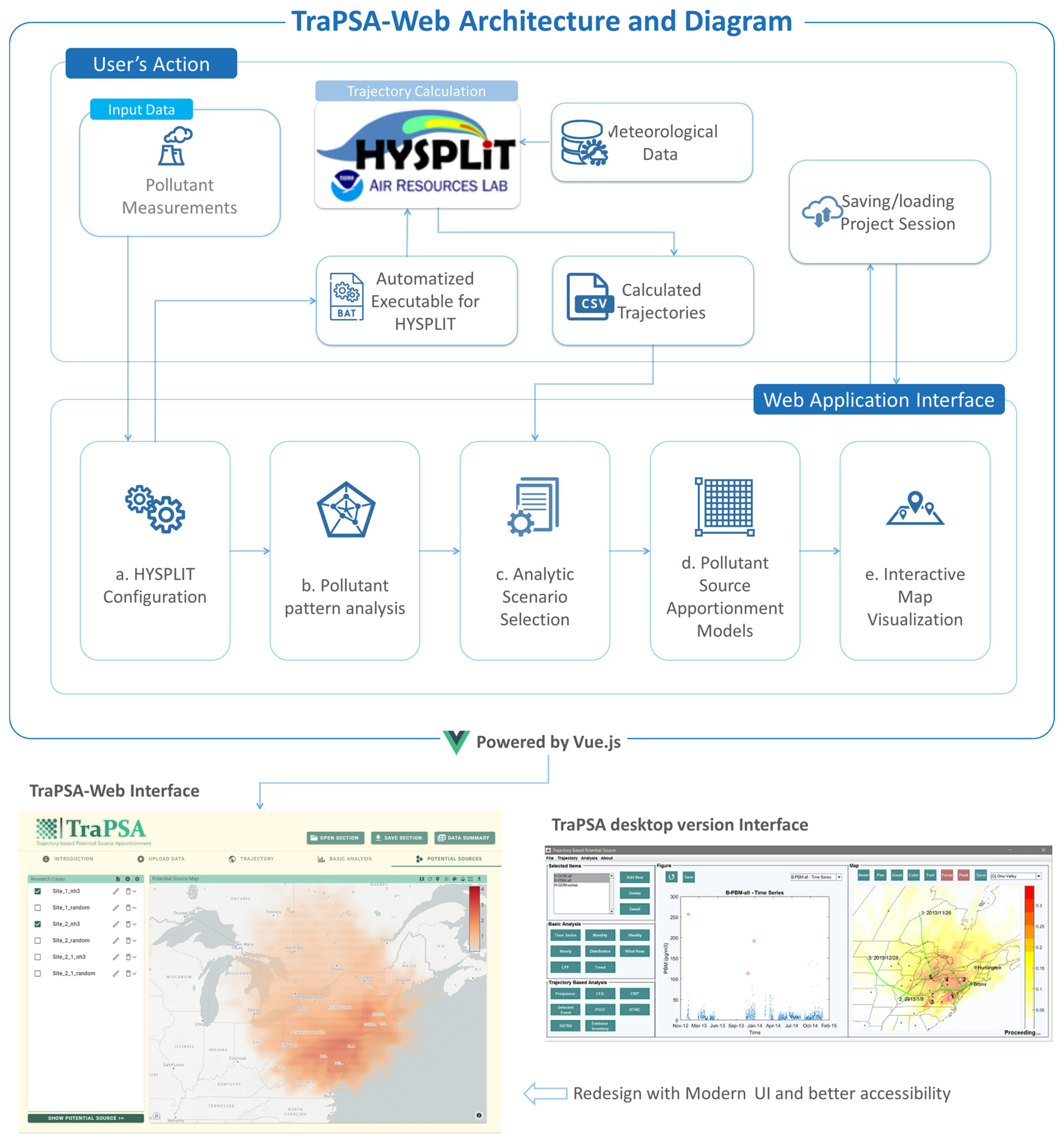
Figure 1 presents a flowchart of the TraPSA-Web application, along with UI comparisons with the desktop version of TraPSA. The pollutant concentration measurement time-series data need to be uploaded to TraPSA-Web. TraPSA-Web requires zero skills to run the HYSPLIT model as it provides easy-to-use HYSPLIT parameter configurations and generates executables (.bat files) for conducting all necessary trajectory calculations with the HYSPLIT model. Note that the generated executables by TraPSA-Web can only support the Windows system and HYSPLIT version 4. This executable also automatically manages and aggregates the HYSPLIT outputs as a single .cvs file. With this aggregated trajectory output file, users can perform TERMs with TraPSA-Web directly or even through other tools, such as Python or MATLAB. Additionally, TraPSA-Web provides functions to save and load projects for future work.
The initial version of TraPSA is a desktop software developed with MATLAB, and it has been applied for multiple research studies across different regions and pollutant species, for example, PM, mercury, and NH3 [5,8,18,19]. The GUI interface of the TraPSA desktop version is shown in Figure 1 (bottom right). The detailed introduction of TraPSA desktop version can be found in Supplementary Materials. To elevate accessibility and user experience, TraPSA was redesigned as a web application with modern UI (depicted in Figure 1, bottom left), which requires no software installation and can be accessed directly through web browsers. TraPSA-Web is developed using Vue.js, a leading front-end web development framework [20].
Unlike desktop software or Python/R packages, TraPSA-Web provides a seamless experience as a pure web application. Users can instantly access the latest version of TraPSA-Web and its new features upon website updates without the need for manual reinstallation or updates on their local systems.
Figure 1. Flowchart of Trajectory-ensemble Potential Source Apportionment Web (TraPSA-Web) application and UI comparisons with the desktop version of TraPSA.
Atmosphere 15 00176 g001
It is important to note that TraPSA-Web does not conduct HYSPLIT trajectory calculations internally. TraPSA-Web generates executables for the automation of performing these calculations locally using HYSPLIT version 4. TraPSA-Web provides guidance for downloading HYSPLIT and the required meteorological data. Other analyses and TERMs were performed using TraPSA-Web. Brief introductions of the TraPSA-Web workflow and examples will be presented in the following sections and a video tutorial with more detailed instructions is available at https://trapsa.netlify.app/ (accessed on 14 November 2023).

2.1. Models Integrated in TraPSA-Web

TraPSA-Web incorporates five of the most widely used TERMs for determining the likely source locations via long-range air transport to the receptor sites. These models were selected based on extensive research comparing the efficiency of TERMs across various scenarios [21,22,23]. These TERMs include Concentration Field Analysis (CFA), Concentration Weighted Trajectory (CWT), Potential Source Contribution Function (PSCF), multiple-site PSCF, and Simplified Quantitative Transport Bias Analysis (SQBA) [24,25,26,27].
These TERMs allocate potential source locations using statistical patterns of air parcel trajectories over a gridded map. In brief, grid cells that are more likely to include pollutant sources tend to correspond with air parcels exhibiting elevated pollutant concentrations. Therefore, the back trajectories originating from high-concentration periods at receptor sites are more likely to traverse those grid cells.
In addition to these trajectory-based models, TraPSA-Web includes wind-based models for more localized source-direction analysis [25,28]. Wind-based models include the Conditional Probability Function (CPF) and Conditional Bivariate Probability Function (CBPF).

2.1.1. CFA and CWT

CFA and CWT were developed to construct a pollutant emission concentration field derived from trajectory endpoints [29,30]. CFA uses logarithmic concentrations for its calculations, making it particularly suitable for pollutants exhibiting significant concentration differences. Conversely, CWT operates using absolute concentrations, which can be used for pollutants with concentrations close to zero [22,24]. The concentration fields of CFA and CWT are defined as follows:
C F i , j = l = 1 L c l τ i , j , l l = 1 L τ i , j , l
where i and j are the grid indices based on latitude and longitude, L represents the total number of back trajectories, c l is the concentration at the starting timestamp of a given back trajectory l, τ i , j , l is the endpoint passing through grids i and j from a given back trajectory l, and C M i , j denotes the concentration field value of grids i, and j with logarithmic concentration applied in CFA and absolute concentration in CWT.

2.1.2. SQTBA

The CFA and CWT allocate the likely pollutant source locations based on the concentration fields, as presented above. However, the accuracy of their source location apportionments might be reduced due to the increased uncertainties that arise with longer trajectory pathways and durations [11,31]. SQTBA is a simplified version of QTBA [1], which accounts for trajectory uncertainties by assuming a normal distribution caused by atmospheric dispersion around the trajectory centerline with a standard deviation that increases linearly with time in the upwind direction. Thus, SQTBA can be used for air pollutant apportionments over larger regions, and the transition probability density function can be expressed as:
Q x , t = 1 2 π σ x ( t ) σ y ( t ) e x p 1 2 X x ( t ) σ x ( t ) 2 + Y y ( t ) σ y ( t ) 2
where X and Y represent the grid center coordinates, x′, y′ are the centerline coordinates of the trajectory, σ is the standard deviation of the trajectories in two directions, which are assumed to grow with time σ x t = σ y t = a t (a is a dispersion speed, equals to 5.4 km/h), and Q x , t is the probability for the air parcel at position x′ at time t′ to arrive at position x at time t.
The potential mass transfer potential field ( T l ¯ x x ) for a given trajectory l arriving at time t is integrated over the back trajectory time τ :
T l ¯ x x = t τ t Q x , t d t t τ t d t
Finally, the SQTBA field is established based on the concentration-weighted mass transfer potential field divided by the potential mass transfer potential field:
S Q T B A x = T ~ x x l = 1 L T l ¯ x x
where c l is the receptor concentration of a given back trajectory l, and L is the total number of back trajectories.

2.1.3. PSCF

The accuracy of the point source location apportionments of concentration field-based models, such as CFA, CWT, and SQTBA, can diminish when the emissions from nonpoint sources are significant [32]. To emphasize the emission impacts from the point source, the PSCF model utilizes only high pollutant concentrations from the receptor sites to calculate conditional probabilities to identify the likely source contribution of each grid to the receptor site [3,6]. A high PSCF value indicates a strong likelihood that the trajectory passing through the grid cell effectively transports contaminants to the receptor site, thereby suggesting a potential emission source location. The PSCF values for a single receptor site are defined as follows:
P S C F i , j = l = 1 L τ i , j , l   |   c l C   l = 1 L τ i , j , l
where C is the criterion concentration to identify high pollutant concentrations (typically set between 75% and 90% of the highest concentration) [18], c l is the concentration at the start of the back trajectory l, L is the total number of back trajectories, and τ i , j , l  is the endpoint that passes through grids i and j from a given back trajectory l. For multiple receptor sites, the PSCF model needs to be adjusted by separating the criterion concentration for each site, as follows [5]:
P S C F i , j = s = 1 S l = 1 L s τ i , j , s , l   |   c s , l   C s s = 1 S l = 1 L s τ i , j , s , l
where S is the total number of sites, C s is the criterion concentration for site s, c s , l is the pollutant concentration of back trajectory l originating from site s, L s is the total number of back trajectories starting from site s, and τ i , j , s , l  is the endpoint that passes through grids i and j from a given back trajectory l starting from site s.

2.1.4. Wind-Based Models

The CPF model determines the probability of a wind direction or speed to be associated with high pollutant levels, and it is defined for a given wind direction θ as follows [25]:
C P F θ = P θ F θ
where P θ is the wind frequency of direction i with high-concentration events, and F θ is the wind frequency of direction i. High-concentration events are identified using a predefined criterion concentration, typically set between 75% and 90% of the highest recorded concentration.
The CBPF model provides a binary conditional probability field based on both wind speed and direction for high-concentrations [8,28]. It is defined as:
C B P F θ , u   = m θ , u |   c > C n θ , u
where m θ , u is the count of high-concentration samples occurring with wind direction at θ and wind speed at u (sample concentration c exceeds criterion concentration C), and n θ , u is the total number of samples in that wind direction and speed. Similar to the CPF model, the criterion concentration is usually set between 75% and 90% of the peak concentration [33].

2.2. TraPSA-Web Interface and Workflows

A typical workflow of an air pollutant source apportionment project with TraPSA-Web is shown in Figure 2. The process involves several key steps: (1) uploading site information, including site name, longitude, latitude, and pollutant measurement time series data to TraPSA-Web, (2) configuring HYSPLIT parameters and generating back trajectory automation executable (.bat file), (3) running the HYSPLIT model using the created .bat file, followed by uploading the aggregated trajectory outputs (.csv file) to TraPSA-Web; (4) establishing analytical scenarios and performing basic analysis; (5) setting parameters for TERMs and visualizing the outcomes; and (6) saving the current project data and configuring for future reference. More detailed guidelines and examples are presented in the following sections. Note that the potential source time series decomposition obtained from positive matrix factorization (PMF) analysis can also be used as the input time series to TraPSA-Web to further improve the likely source apportionment [3,18].

2.3. Future Updates

The planned future updates for TraPSA-Web encompass (1) integrating support to the newest HYSPLIT version, (2) incorporating additional TERMs and advanced trajectory statistical analyses, such as 3D-PSCF [34], and Potential Source Density Function [35], (3) improving visualization flexibility and diversity of visualization options, (4) enhancing the computational efficiency of TERMs calculations and map visualizations, and (5) expanding the range of output formats for TERM results to include formats like TIFF files and GeoJSON.

3. Example of Toolkit Application

The following sections will present a detailed example project demonstrating the power of TraPSA-Web in conducting likely source location apportionment with TERMs and HYSPLIT. This example will highlight TraPSA-Web’s capabilities and effectiveness in addressing the core challenges inherent in TERM analyses, including automation of trajectory calculations and management, analyzing the seasonality of the likely source locations [8], and reducing the “trailing effect” [2].
This example uses atmospheric ammonia (NH3) concentration data measured at two sites in New York State from 2016 to 2017. The two sites are located in New York City (40.73614, −73.82153) and Potsdam (44.662118, −75.001016). The example dataset is available at https://trapsa.netlify.app/example_data.rar (accessed on 14 November 2023), and the example project is available at https://trapsa.netlify.app/example.trapsa (accessed on 14 November 2023).

3.1. Data and Project Management

TraPSA-Web requires specific input data for receptor site information, pollutant concentration measurements, and wind speed and direction. Site information is uploaded via a .csv file with fixed header names: “site_name,” “lat,” and “lon.” Successful uploads are confirmed with a table displaying site details and a map pinpointing the site locations. For instance, uploading the “site.csv” file imports sites named Potsdam and Queen’s College into TraPSA-Web, as illustrated in Figure 2(1) (top).
Subsequently, time series data for each site, including pollutants, wind speed, and directions, were uploaded through separate or combined .csv files. TraPSA-Web offers flexibility in header names for time series data. The meaning of header names can be assigned by categorizing them under “Timestamp,” “Site Name,” “Measurements,” “Wind Direction,” and “Wind Speed” through dragging and dropping operations. Only “Timestamp,” “Site Name,” and “Measurements” are mandatory, and the rows with missing values will be excluded from the following analysis. The correct data upload is also verified through a data table display similar to the site information upload. By uploading the “all_combined.csv” file, the NH3 measurement concentrations and randomly generated concentrations of the two sites are imported to TraPSA-Web, as illustrated in Figure 2(1) (bottom).
Project progress can be saved using the “Save Session” button (Figure 2(6)), generating a .trapsa file with all project data and settings. This file can be reloaded with the “Open Session” button to retrieve the saved project progress. The “Data Summary” feature allows for viewing and managing site data, measurement data, and trajectory endpoint data.

3.2. Configure Back Trajectory Automation

To perform TERMs, the back trajectory needs to be configured and calculated for each measurement timestamp. This configuration workload can be high due to the potentially large number of timestamps. TraPSA-Web simplifies this task with a user-friendly GUI, generating automation executables (.bat file) that conduct HYSPLIT calculations and output management. The HYSPLIT parameters configurable in TraPSA-Web include the back trajectory time, starting height, starting height type, and meteorological data type.
TraPSA-Web also provides up-sampling of the timestamp for the trajectory calculation to address the application of TERMs in air pollutants with low temporal resolutions. For example, if the pollutant is measured every 24 h, TraPSA-Web can generate multiple trajectories within 24 h to provide more complete pollutant transportation situations by configuring the “data sampling period” and “up-sampling number.”
Various meteorological data formats compatible with HYSPLIT are supported by TraPSA-Web. Typically, the Eta Data Assimilation System (EDAS) with 40 km resolution data [36] and North American Regional Reanalysis (NARR) data with 32 km resolution are used for the North American region [25,37]. The Global Data Assimilation System (GDAS) [38] and the NCEP/NCAR Reanalysis Archive with 2.5-degree resolution can be used globally [39,40]. GDAS provides various spatial resolutions, including 0.25° × 0.25°, 0.5° × 0.5°, and 1° × 1°. The fifth-generation ECMWF reanalysis (ERA5) with 2.5-degree resolution can also be used for global analysis [41]; however, the support for ERA5 of TraPSA-Web is still under development. The starting years for EDAS, NARR, GDAS, NCEP/NCAR, and ERA5 were 2004, 1979, 2001, 1948, and 1940, respectively.
In our example, using hourly NH3 measurements, trajectory up-sampling was not used. The back trajectory duration was set to 24 h (Figure 2(2)) due to the relatively short lifetime of atmospheric NH3 [42], and the starting point was set to 500 m above the ground, similar to most of the previous studies. The NCEP/NCAR Reanalysis Archive was used as the meteorological data. An automation executable file, “run_HYSPLIT.bat,” was generated and downloaded for conducting the HYSPLIT model, producing a .csv file containing the aggregated trajectory endpoints upon execution (Figure 2(3)).

3.3. Analytical Scenarios

Pollutant concentration patterns and source locations can vary due to factors like mitigation efforts or seasonal emission changes [5,8,27]. Therefore, it is important to analyze the likely source locations for different scenarios and periods. TraPSA-Web enables customization of analytical scenarios based on timeframes, seasonality, and diurnal periods (Figure 2(4)). Significant NH3 likely source location shifts can be observed from the PSCF model results for New York City across different seasons, as shown in Figure 3. TraPSA-Web also offers the basic analysis for user-defined scenarios, including concentration distributions, time series, diel patterns, seasonal patterns, trends, wind rose, CPF, and CBPF (Figure 2(4)).

3.4. Configure Grid Sizes and Weights for TERMs

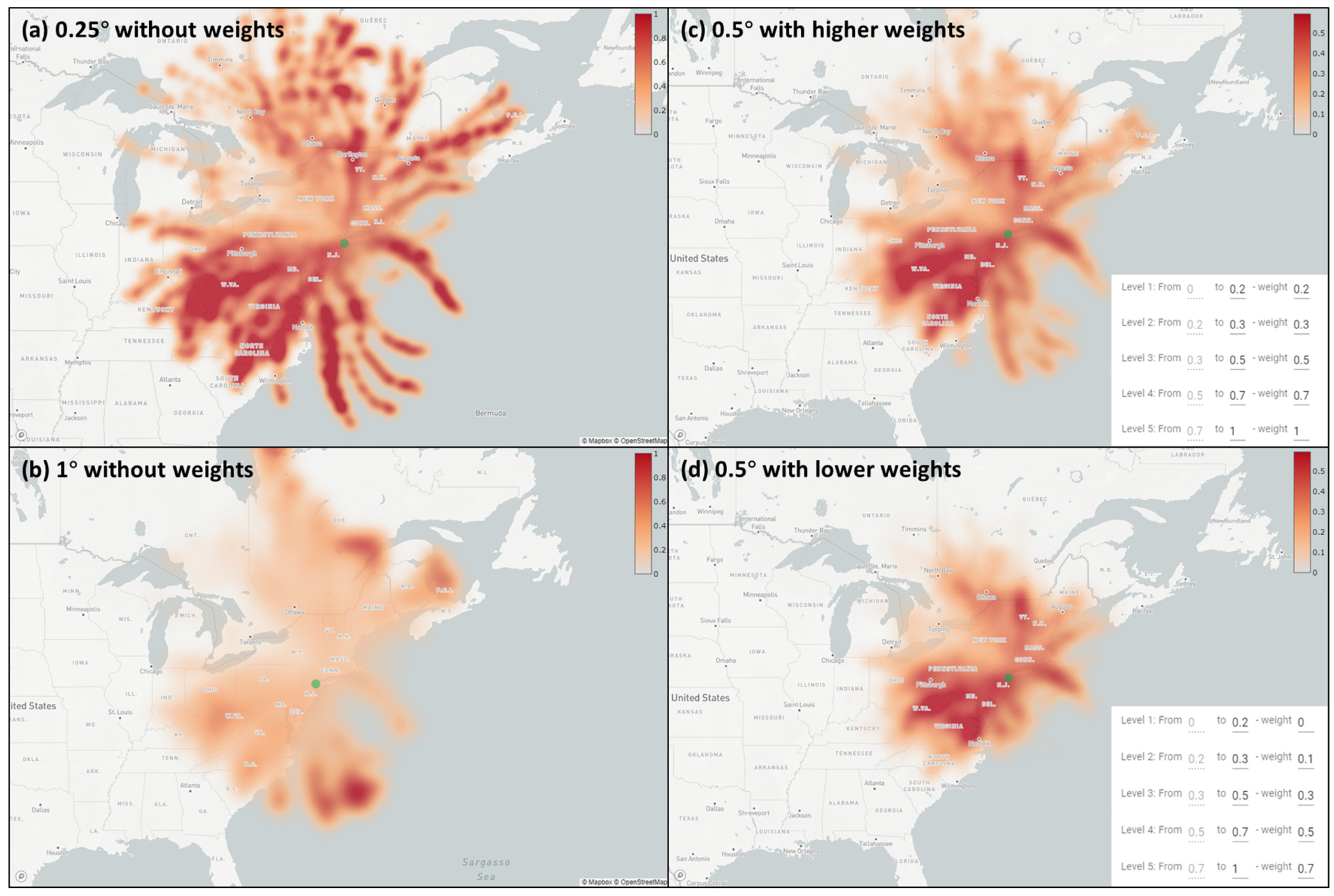
The “trailing effect” is the false source locations identified due to sparse trajectory crossings [2]. This can be mitigated by choosing proper grid sizes or applying grid weighting functions to reduce the impacts from grids with fewer trajectory endpoints. The grid sizes and weights were both adjustable in TraPSA-Web (Figure 2(5)). The grid weighting function is defined as follows:
w i , j = p 1 | n i , j a v g < l 1 p 2 | l 1 < n i , j a v g < l 2 p k | l k 1 < n i , j a v g < l k
where w i , j is the grid weight for grids i j, n i , j are the endpoint counts of grids i and j, avg is the average endpoint number across all grid cells (total endpoints/grid number), p k are the weight factors for level k, and l k are the endpoint ratio ranges for level k. The weight factor ( p k ) in TraPSA-Web was set to 1 for the grids exceeding the highest weight level ( l k ).
Figure 4 compares the “trailing effect” in the PSCF model results for New York City with different grid sizes and weight configurations. The figure demonstrates that increasing the grid size can effectively mitigate the “trailing effect” (as evident in Figure 4a,b). However, a coarse grid size reduces the confidence of the likely source identified. In the example project, a grid size of 0.5° × 0.5° was selected to balance between spatial resolution and the confidence of source location detection. As shown in Figure 4c,d, the “trailing effect” can be further reduced by lowering the weights of the grid with small trajectory endpoint numbers, presenting clear likely source locations. The configurations for grid sizes and weights in TraPSA-Web though can be arbitrary based on previous studies and project domain knowledge, are crucial in the process of likely source apportionment using TERMs. These parameters play a pivotal role in balancing meaningful signals and background noise of the TERMs, ensuring the clarity and accuracy of the final likely source maps.

3.5. Comparisons and Visualizations

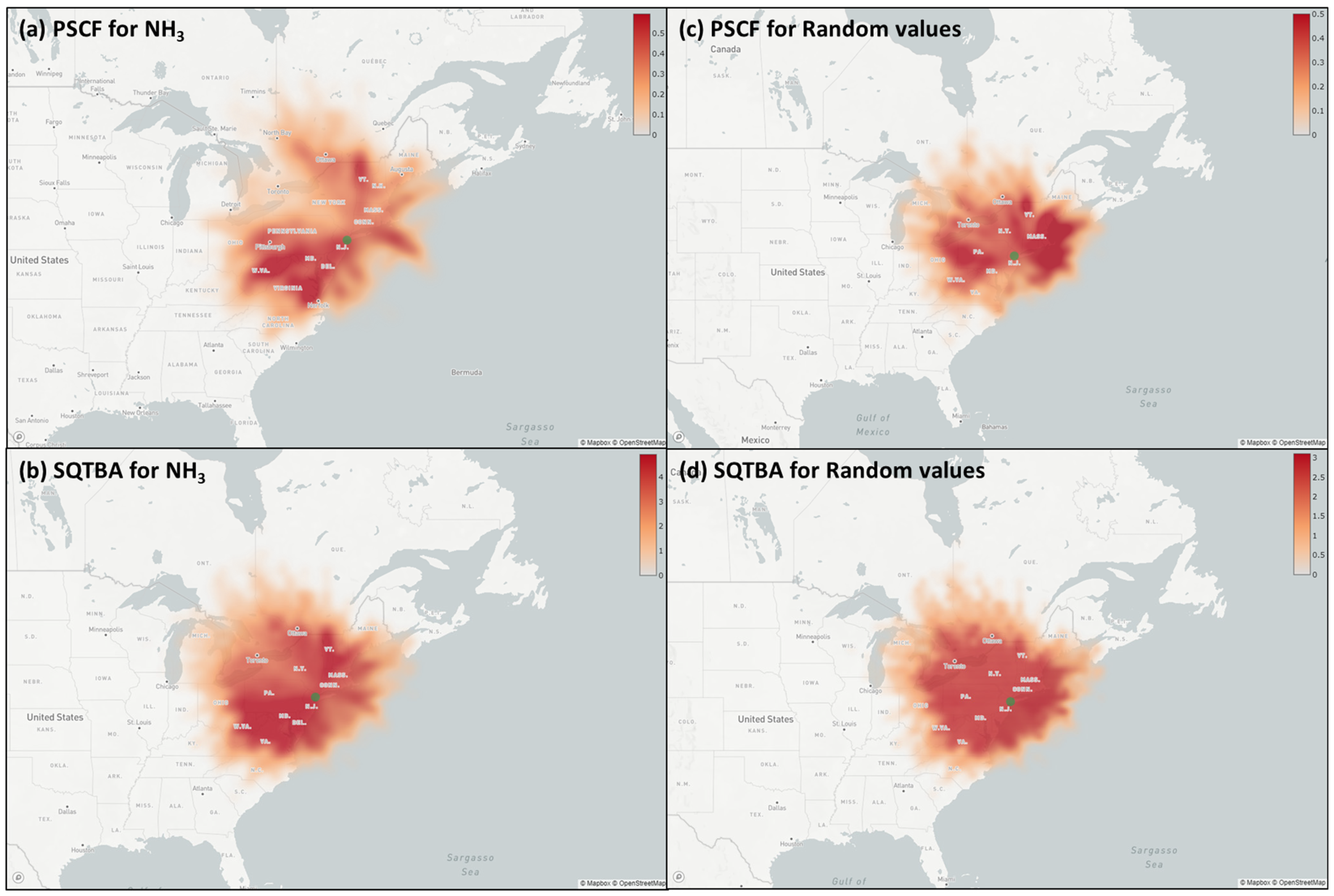
As discussed above, the concentration criterion-based TERMs, for example, PSCF, only link pollutant measurements with high-concentrations to source emissions through the back trajectory. Therefore, they can provide clear separations for the likely source locations, which is good for apportionments for point-source locations. On the contrary, concentration field-based TERMs, such as CFA, CWT, and SQTBA, consider all pollutant measurements equally, and they can provide more complete pollutant emission pictures. Comparisons between the PSCF and SQTBA are shown in Figure 5. The visualizations can be improved by adjusting the colormaps, opacity, and smoothness using interactive map tools provided by TraPSA-Web.
The PSCF and SQTBA models were applied to NH3 measurements and randomly generated concentration values with a normal distribution. Randomly generated values were designed to test the models’ robustness by providing a “zero-source” case. As shown in Figure 5a,b, the PSCF results provided better separations for the likely source locations than SQTBA for NH3. However, PSCF detected “fake source” locations (Figure 5c) while SQTBA generated a unique concentration field (Figure 5d) that indicates no significant emission sources or equal emission contributions within the region, which is better aligned with the “zero-source” assumption. Therefore, similar to the configuration of grid weights, there is also a trade-off between signal and noise in the model selection, requiring project domain knowledge, such as the physic-chemical characteristics of the target pollutants and potential pollutant source information within the research regions.
Figure 5. Demonstrations of the efficacy of PSCF and SQTBA analyses for likely source location apportionments. The likely source locations of NH3 measurements in the New York City site (green dots) can be identified in (a,b). Conversely, no clear source locations can be found in the outputs of randomly generated time series, as evidenced in (c,d).
Atmosphere 15 00176 g005

4. Software and Data Availability

The TraPSA-Web (version 1.0) is available at https://trapsa.netlify.app/ (accessed on 14 November 2023). The full tutorials and example datasets to further demonstrate the capabilities of the TraPSA-web application can be found in Supplementary Materials.

5. Conclusions

This paper presents TraPSA-Web, an innovative web-based application offering the air quality research community a comprehensive, flexible, and user-friendly platform for atmospheric pollutant source apportionments. TraPSA-Web is designed to streamline the process of likely source location identifications using TERMs and HYSPLIT. TraPSA-Web provides the following key functionalities that enhance the TERM analysis processes: (1) easy-to-use project and data management, (2) automated HYSPLIT back trajectory configuration, calculation, and results processing, (3) customizable analytical scenarios and comprehensive TERM analysis, (4) interactive data and map visualization, and (5) instantly access the latest version through a web browser. The example project presented in this paper demonstrates that TraPSA-Web can significantly reduce the complexity and time required for TERM analyses with its modern GUI, highly automated analysis procedures, and sophisticated analyses.

Supplementary Materials

The following supporting information can be downloaded at: https://trapsa.netlify.app/ (accessed on 14 November 2023). The TraPSA-web tutorial video is available at https://player.vimeo.com/video/542644809 (accessed on 14 November 2023). Example datasets of TraPSA-Web are available at https://trapsa.netlify.app/example_data.rar (accessed on 14 November 2023). An example project of TraPSA-Web is available at https://trapsa.netlify.app/example.trapsa (accessed on 14 November 2023). The source code of TraPSA-Web is available at https://github.com/defve1988/TraPSA_vue (accessed on 14 November 2023). The TraPSA desktop version is available at https://webspace.clarkson.edu/projects/TraPSA/public_html/ (accessed on 23 January 2024). The algorithms of trajectory ensemble receptor models and the instructions for the TraPSA desktop version are available at https://webspace.clarkson.edu/projects/TraPSA/public_html/en/userguide.html (accessed on 14 November 2023).

Author Contributions

C.Z. developed the TraPSA-Web; H.Z. assisted in the testing and evaluation of TraPSA; P.K.H. and T.M.H. contributed to the concept of the TraPSA project and trajectory ensemble receptor models. All authors have read and agreed to the published version of the manuscript.

Funding

This research received no external funding.

Institutional Review Board Statement

Not applicable.

Informed Consent Statement

Not applicable.

Data Availability Statement

Data is contained within the article or Supplementary Materials.

Acknowledgments

The authors would like to thank the reviewers and editors for their dedication and valuable input in improving this manuscript. The authors extend their sincere gratitude to Mark Cohen of NOAA Air Resources Laboratory for his valuable support in the HYSPLIT model.

Conflicts of Interest

The authors declare no conflict of interest.

References

  1. Hopke, P.K. Review of Receptor Modeling Methods for Source Apportionment. J. Air Waste Manag. Assoc. 2016, 6, 237–259. [Google Scholar] [CrossRef] [PubMed]
  2. Cheng, I.; Xu, X.; Zhang, L. Overview of Receptor-Based Source Apportionment Studies for Speciated Atmospheric Mercury. Atmos. Chem. Phys. 2015, 15, 7877–7895. [Google Scholar] [CrossRef]
  3. Gao, Y.; Lyu, T.; Zhang, W.; Zhou, X.; Zhang, R.; Tang, Y.; Jiang, Y.; Cao, H. Control Priority Based on Source-Specific DALYs of PM2.5-Bound Heavy Metals by PMF-PSCF-IsoSource Model in Urban and Suburban Beijing. J. Environ. Manag. 2024, 352, 120016. [Google Scholar] [CrossRef] [PubMed]
  4. Dai, M.; Liu, A.; Sheng, Y.; Xian, Y.; Wang, H.; Wang, C. Analysis of PM2.5 Characteristics in Yancheng from 2017 to 2021 Based on Kolmogorov–Zurbenko Filter and PSCF Model. Atmosphere 2023, 14, 317. [Google Scholar] [CrossRef]
  5. Zhou, H.; Zhou, C.; Lynam, M.M.; Dvonch, J.T.; Barres, J.A.; Hopke, P.K.; Cohen, M.; Holsen, T.M. Atmospheric Mercury Temporal Trends in the Northeastern United States from 1992 to 2014: Are Measured Concentrations Responding to Decreasing Regional Emissions? Environ. Sci. Technol. Lett. 2017, 4, 91–97. [Google Scholar] [CrossRef]
  6. Ren, B.; Xie, P.; Xu, J.; Li, A.; Tian, X.; Hu, Z.; Huang, Y.; Li, X.; Zhang, Q.; Ren, H.; et al. Use of the PSCF Method to Analyze the Variations of Potential Sources and Transports of NO2, SO2, and HCHO Observed by MAX-DOAS in Nanjing, China during 2019. Sci. Total Environ. 2021, 782, 146865. [Google Scholar] [CrossRef]
  7. Salmabadi, H.; Saeedi, M. Determination of the Transport Routes of and the Areas Potentially Affected by SO2 Emanating from Khatoonabad Copper Smelter (KCS), Kerman Province, Iran Using HYSPLIT. Atmos. Pollut. Res. 2019, 10, 321–333. [Google Scholar] [CrossRef]
  8. Zhou, C.; Zhou, H.; Holsen, T.M.; Hopke, P.K.; Edgerton, E.S.; Schwab, J.J. Ambient Ammonia Concentrations Across New York State. J. Geophys. Res. D Atmos. 2019, 124, 8287–8302. [Google Scholar] [CrossRef]
  9. Shen, L.; Wang, H.; Kong, X.; Zhang, C.; Shi, S.; Zhu, B. Characterization of Black Carbon Aerosol in the Yangtze River Delta, China: Seasonal Variation and Source Apportionment. Atmos. Pollut. Res. 2021, 12, 195–209. [Google Scholar] [CrossRef]
  10. Dehshiri, S.S.H.; Firoozabadi, B.; Afshin, H. A New Application of Multi-Criteria Decision Making in Identifying Critical Dust Sources and Comparing Three Common Receptor-Based Models. Sci. Total Environ. 2022, 808, 152109. [Google Scholar] [CrossRef]
  11. Stein, A.F.; Draxler, R.R.; Rolph, G.D.; Stunder, B.J.B.; Cohen, M.D.; Ngan, F. NOAA’s HYSPLIT Atmospheric Transport and Dispersion Modeling System. Bull. Am. Meteorol. Soc. 2015, 96, 2059–2077. [Google Scholar] [CrossRef]
  12. Stohl, A. The FLEXTRA Trajectory Model Version 3.0 User Guide. Available online: https://www.flexpart.eu/wiki (accessed on 14 November 2023).
  13. Zeng, J.; Matsunaga, T.; Mukai, H. METEX—A Flexible Tool for Air Trajectory Calculation. Environ. Model. Softw. 2010, 25, 607–608. [Google Scholar] [CrossRef]
  14. Zhang, Y.; Xu, H.; Zhang, Y.; Luo, J.; Chen, F.; Cao, B.; Xie, M. Analysis of Air Pollutants and Their Potential Sources in Eastern Xinjiang, Northwestern Inland China, from 2018 to 2022. Atmosphere 2023, 14, 1670. [Google Scholar] [CrossRef]
  15. Wang, Y.Q.; Zhang, X.Y.; Draxler, R.R. TrajStat: GIS-Based Software That Uses Various Trajectory Statistical Analysis Methods to Identify Potential Sources from Long-Term Air Pollution Measurement Data. Environ. Model. Softw. 2009, 24, 938–939. [Google Scholar] [CrossRef]
  16. Carslaw, D.C.; Ropkins, K. Openair—An R Package for Air Quality Data Analysis. Environ. Model. Softw. 2012, 27, 52–61. [Google Scholar] [CrossRef]
  17. Weber, S. pyPSCF. Available online: https://pypi.org/project/pyPSCF/ (accessed on 14 November 2023).
  18. Zhou, H.; Hopke, P.K.; Zhou, C.; Holsen, T.M. Ambient Mercury Source Identification at a New York State Urban Site: Rochester, NY. Sci. Total Environ. 2019, 650, 1327–1337. [Google Scholar] [CrossRef]
  19. Shanavas, A.K.; Zhou, C.; Menon, R.; Hopke, P.K. PM10 Source Identification Using the Trajectory Based Potential Source Apportionment (TraPSA) Toolkit at Kochi, India. Atmos. Pollut. Res. 2020, 11, 1535–1542. [Google Scholar] [CrossRef]
  20. Vue.js—The Progressive JavaScript Framework. Available online: https://vuejs.org/ (accessed on 17 November 2023).
  21. Liu, J.; Li, J.; Yao, F. Source-Receptor Relationship of Transboundary Particulate Matter Pollution between China, South Korea and Japan: Approaches, Current Understanding and Limitations. Crit. Rev. Environ. Sci. Technol. 2022, 52, 3896–3920. [Google Scholar] [CrossRef]
  22. Kabashnikov, V.P.; Chaikovsky, A.P.; Kucsera, T.L.; Metelskaya, N.S. Estimated Accuracy of Three Common Trajectory Statistical Methods. Atmos. Environ. 2011, 45, 5425–5430. [Google Scholar] [CrossRef]
  23. And, Y.-J.H.; Holsen, T.M.; Hopke, P.K.; Yi, S.-M. Comparison between Back-Trajectory Based Modeling and Lagrangian Backward Dispersion Modeling for Locating Sources of Reactive Gaseous Mercury. Environ. Sci. Technol. 2005, 39, 1715–1723. [Google Scholar] [CrossRef]
  24. Cheng, I.; Zhang, L.; Blanchard, P.; Dalziel, J.; Tordon, R. Concentration-Weighted Trajectory Approach to Identifying Potential Sources of Speciated Atmospheric Mercury at an Urban Coastal Site in Nova Scotia, Canada. Atmos. Chem. Phys. 2013, 13, 6031–6048. [Google Scholar] [CrossRef]
  25. Squizzato, S.; Masiol, M. Application of Meteorology-Based Methods to Determine Local and External Contributions to Particulate Matter Pollution: A Case Study in Venice (Italy). Atmos. Environ. 2015, 119, 69–81. [Google Scholar] [CrossRef]
  26. Zhao, N.; Wang, G.; Li, G.; Lang, J.; Zhang, H. Air Pollution Episodes during the COVID-19 Outbreak in the Beijing–Tianjin–Hebei Region of China: An Insight into the Transport Pathways and Source Distribution. Environ. Pollut. 2020, 267, 115617. [Google Scholar] [CrossRef]
  27. Abdo, S.; Koroleva, Y. Seasonal Characteristics of Long-Range Transport and Potential Associated Sources of Particulate Matter (PM10) Pollution at the Station Elk, Poland, on 2021–2022 Data. Geogr. Environ. Sustain. 2023, 16, 92–101. [Google Scholar] [CrossRef]
  28. Nguyen, T.N.T.; Vuong, Q.T.; Lee, S.-J.; Xiao, H.; Choi, S.-D. Identification of Source Areas of Polycyclic Aromatic Hydrocarbons in Ulsan, South Korea, Using Hybrid Receptor Models and the Conditional Bivariate Probability Function. Environ. Sci. Process. Impacts 2022, 24, 140–151. [Google Scholar] [CrossRef] [PubMed]
  29. Rutter, A.P.; Snyder, D.C.; Stone, E.A.; Schauer, J.J.; Gonzalez-Abraham, R.; Molina, L.T.; Márquez, C.; Cárdenas, B.; de Foy, B. In Situ Measurements of Speciated Atmospheric Mercury and the Identification of Source Regions in the Mexico City Metropolitan Area. Atmos. Chem. Phys. 2009, 9, 207–220. [Google Scholar] [CrossRef]
  30. Weiss-Penzias, P.S.; Gustin, M.S.; Lyman, S.N. Sources of Gaseous Oxidized Mercury and Mercury Dry Deposition at Two Southeastern U.S. Sites. Atmos. Environ. 2011, 45, 4569–4579. [Google Scholar] [CrossRef]
  31. Pérez, I.A.; Artuso, F.; Mahmud, M.; Kulshrestha, U.; Sánchez, M.L.; García, M.Á. Applications of Air Mass Trajectories. Adv. Meteorol. 2015, 2015, 284213. [Google Scholar] [CrossRef]
  32. Berriban, I.; Azahra, M.; Chham, E.; Ferro-García, M.A.; Milena-Pérez, A.; Nouayti, A.; Orza, J.A.G.; Brattich, E.; Tositti, L.; Piñero-García, F.; et al. PSCF and CWT Methods as a Tool to Identify Potential Sources of 7Be and 210Pb Aerosols in Granada, Spain. J. Environ. Radioact. 2022, 251–252, 106977. [Google Scholar] [CrossRef] [PubMed]
  33. Uria-Tellaetxe, I.; Carslaw, D.C. Conditional Bivariate Probability Function for Source Identification. Environ. Model. Softw. 2014, 59, 1–9. [Google Scholar] [CrossRef]
  34. Dimitriou, K.; Grivas, G.; Liakakou, E.; Gerasopoulos, E.; Mihalopoulos, N. Assessing the Contribution of Regional Sources to Urban Air Pollution by Applying 3D-PSCF Modeling. Atmos. Res. 2021, 248, 105187. [Google Scholar] [CrossRef]
  35. Kim, I.S.; Kim, Y.P.; Wee, D. Potential Source Density Function: A New Tool for Identifying Air Pollution Sources. Aerosol Air Qual. Res. 2022, 22, 210236. [Google Scholar] [CrossRef]
  36. NOAA Air Resources Laboratory. EDAS 40 km Data Archive. Available online: https://www.ready.noaa.gov/edas40.php (accessed on 22 January 2024).
  37. NOAA National Centers for Environmental Information. North American Regional Reanalysis. Available online: https://www.ncei.noaa.gov/products/weather-climate-models/north-american-regional (accessed on 22 January 2024).
  38. NOAA National Centers for Environmental Information. Global Data Assimilation System (GDAS). Available online: https://www.ncei.noaa.gov/access/metadata/landing-page/bin/iso?id=gov.noaa.ncdc:C00379 (accessed on 22 January 2024).
  39. NOAA Air Resources Laboratory. NCEP/NCAR Global Reanalysis Data Archive. Available online: https://www.ready.noaa.gov/gbl_reanalysis.php (accessed on 22 January 2024).
  40. Fu, X.W.; Feng, X.; Liang, P.; Deliger; Zhang, H.; Ji, J.; Liu, P. Temporal Trend and Sources of Speciated Atmospheric Mercury at Waliguan GAW Station, Northwestern China. Atmos. Chem. Phys. 2012, 12, 1951–1964. [Google Scholar] [CrossRef]
  41. Hersbach, H.; Bell, B.; Berrisford, P.; Biavati, G.; Horányi, A.; Muñoz Sabater, J.; Nicolas, J.; Peubey, C.; Radu, R.; Rozum, I. ERA5 Hourly Data on Single Levels from 1979 to Present, Copernicus Climate Change Service (c3s) Climate Data Store (cds). Available online: https://cds.climate.copernicus.eu/cdsapp#!/dataset/reanalysis-era5-single-levels?tab=overview (accessed on 22 January 2024). [CrossRef]
  42. Tang, Y.S.; Braban, C.F.; Dragosits, U.; Dore, A.J.; Simmons, I.; van Dijk, N.; Poskitt, J.; Dos Santos Pereira, G.; Keenan, P.O.; Conolly, C.; et al. Drivers for Spatial, Temporal and Long-Term Trends in Atmospheric Ammonia and Ammonium in the UK. Atmos. Chem. Phys. 2018, 18, 705–733. [Google Scholar] [CrossRef]
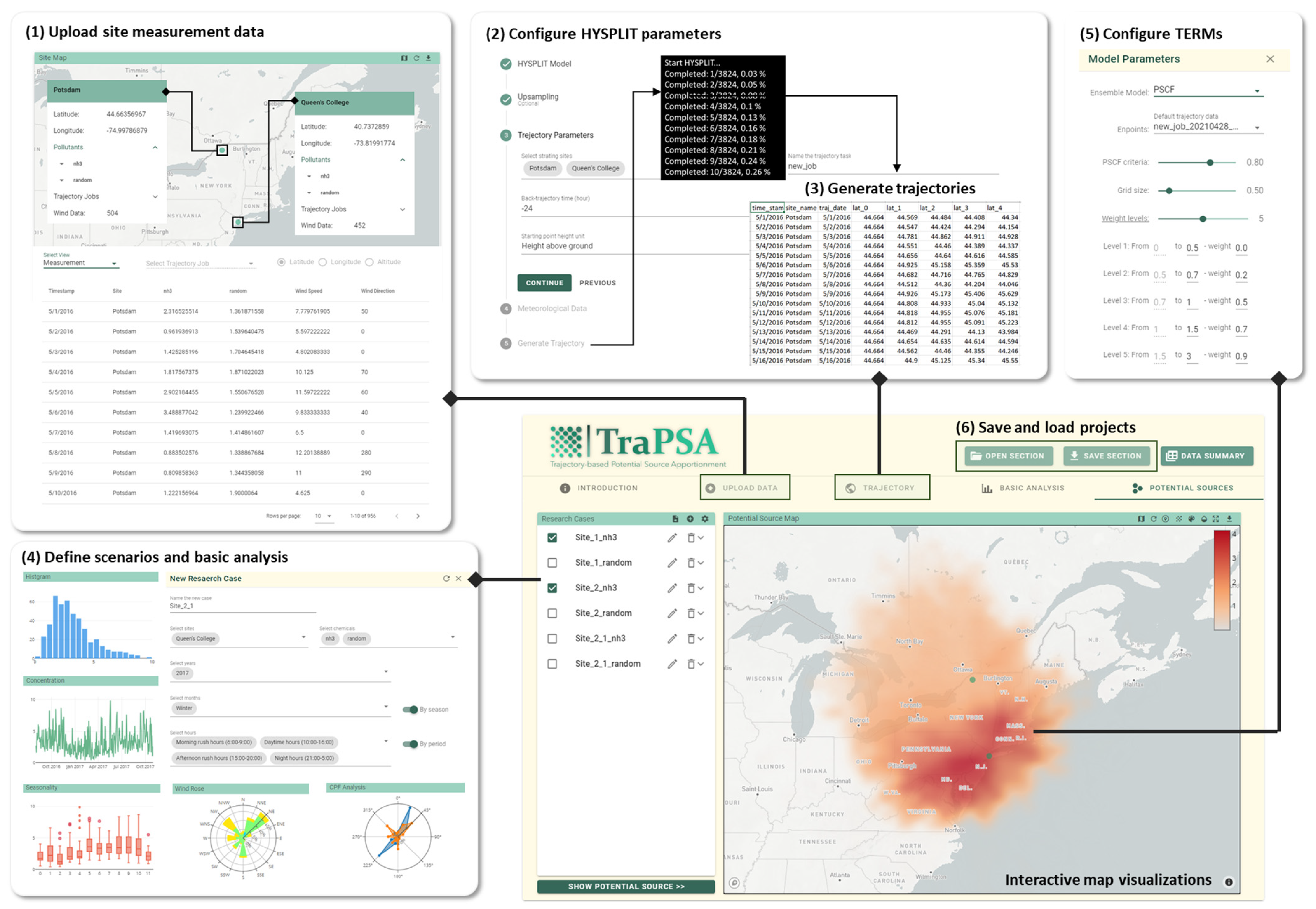
Figure 2. Interface and workflows of Trajectory-ensemble Potential Source Apportionment Web (TraPSA-Web) application.
Atmosphere 15 00176 g002
Figure 3. Example outputs of TraPSA-Web depicting the seasonality of likely source locations. The PSCF model results of NH3 measurements from the New York City site (green dots) for different seasons are shown in (a) Spring, (b) Summer, (c) Autumn, and (d) Winter.
Atmosphere 15 00176 g003
Figure 4. Examples of reducing the “trailing effect” by properly configuring grid size and weights in TraPSA-Web. The “trailing effect” can affect the likely source location apportionment, as shown in (a,b). This effect can be reduced by configuring the grid size and weighting function in TraPSA-Web, as shown in (c,d). The grid sizes and weight configurations are shown in the figures. The green dots present the monitoring site locations.
Atmosphere 15 00176 g004
Disclaimer/Publisher’s Note: The statements, opinions and data contained in all publications are solely those of the individual author(s) and contributor(s) and not of MDPI and/or the editor(s). MDPI and/or the editor(s) disclaim responsibility for any injury to people or property resulting from any ideas, methods, instructions or products referred to in the content.