Abstract
An array of SuperDARN meteor radars at northern high latitudes was used to investigate the sources and characteristics of eastward-propagating planetary waves (EPWs) at 95 km, with a focus on wintertime. The nine radars provided the daily mean meridional winds and their anomalies over 180 degrees of longitude, and these anomalies were separated into eastward and westward waves using a fast Fourier transform (FFT) method to extract the planetary wave components of zonal wavenumbers 1 and 2. Years when a sudden stratospheric warming event with an elevated stratopause (ES-SSW) occurred during the winter were contrasted with years without such events and composited through superposed epoch analysis. The results show that EPWs are a ubiquitous—and unexpected—feature of meridional wind variability near 95 km. Present even in non-ES-SSW years, they display a regular annual cycle peaking in January or February, depending on the zonal wavenumber. In years when an ES-SSW occurred, the EPWs were highly variable but enhanced before and after the onset.
1. Introduction
Eastward-propagating planetary waves (EPWs), that is, planetary waves propagating eastward relative to a ground observer, have long been observed at high latitudes during the winter in satellite and radar observations of the middle atmosphere. According to the Charney–Drazin criterion governing one-dimensional vertical propagation of planetary waves (PWs) through a constant zonal wind, troposphere-sourced EPWs can propagate through faster eastward background winds than quasi-stationary waves [1]. On the other hand, such EPWs could also be generated in situ in the middle atmosphere. Overall, EPWs have been much less studied than their quasi-stationary and westward-propagating counterparts.
As the background eastward zonal wind decays with altitude in the high-latitude mesosphere/lower thermosphere (MLT), upward-propagating EPWs are primarily vertically confined by a critical level, at which their refractive index tends to infinity, where they dissipate. However, EPWs can also be generated from unstable flows in the MLT [2,3]. The necessary condition for in situ planetary wave growth due to instability is that a critical level lies just beyond a turning level, i.e., a level at which the meridional potential vorticity gradient changes sign and the refractive index becomes imaginary. At such a turning level, a planetary wave becomes evanescent and decays with height. However, if the wave can tunnel to its adjoining critical level, it can reverse its propagation direction and grow in amplitude by extracting energy from the background flow, i.e., it can over-reflect. The concept of over-reflection has previously been described [4] and applied to study the interactions among incident, transmitted, and reflected planetary waves in the stratosphere [5]. The existence of such a turning level arises from the dissipation of upward-propagating gravity waves capping the eastward wintertime mean flow and inducing vertical shear and curvature.
As a possible origin for EPWs, early model studies primarily investigated the barotropic instability using linear [6,7] or fully nonlinear models [8], as well as a general circulation model [9]. A double eastward jet was also identified as a possible source of instability for generating eastward-propagating 4-day waves [8,10]. Such a double-jet meridional profile, formed by the polar night jet and the mesospheric subtropical jet, is a configuration that commonly appears before the occurrence of a stratospheric sudden warming (SSW) in the northern hemisphere (NH) [3,11]. Satellite temperature observations by the Microwave Limb Sounder (MLS) revealed a wave-2 EPW (hereafter EPW-2) in the NH prior to the onset of the January 2009 SSW [12]. This finding was supported in a case study of this event [3] using the Whole Atmosphere Community Climate Model (WACCM) nudged by Modern-Era Retrospective Analysis for Research and Applications, version 2 (hereafter MERRA-2) reanalyses [13]. More recently, other occurrences of EPWs surrounding several SSW events were reported from MLS observations [14]. The in situ generation of EPWs surrounding SSW events was also found in WACCM model ensemble simulations [5].
A recent study [2] combined Sounding of the Atmosphere using Broadband Emission Radiometry (SABER) temperature observations and MERRA-2 re-analyses from 2002–2018, suggesting that EPWs are ubiquitous in the NH winter polar mesosphere. With long periods (10–40 days), these EPWs thus appear much more often than just prior to SSWs. They were inferred to be maintained by the shear instability in the lower mesosphere and to provide an eastward acceleration at the level they are emitted, near 60–80 km, compensating for the local westward acceleration provided by the dissipating quasi-stationary PWs. These EPWs could subsequently propagate downward from their generation region into the stratosphere, or upward into the upper mesosphere, depending on the mean flow structure and wave characteristics. Ultimately, they exert a westward acceleration, where they dissipate. The identified balance between the opposite accelerations provided by the EPW generation and the quasi-stationary PW dissipation in the lower mesosphere [2] points to an essential role of the ubiquitous EPWs in maintaining the zonal momentum balance.
In this study, we detected the ubiquitous presence of long-period (4–30 days) EPWs in the MLT from novel observations by a network of SuperDARN radars in the high latitudes of the NH. This was achieved by deriving meridional winds near 95 km from hourly radar observations of meteor winds and by fitting PWs with zonal wavenumbers 1 and 2 (hereafter S1 and S2, respectively) across longitudes [15,16,17]. The eastward-propagating components, hereafter EPW-S1 and EPW-S2, were further extracted by two-dimensional fast Fourier transform (2D-FFT).
2. Data and Methodology
2.1. Data Source
Data from a network of high-frequency, ground-based radars known as the Super Dual Auroral Radar Network (SuperDARN) [15,18,19,20] were used from their meteor–radar mode. A map of the 10 SuperDARN radar sites has previously been shown [21]. For further details about the individual radars and their characteristics, see the Data Availability statement below.
In this study, we retained data from nine northern hemisphere SuperDARN radars along the latitude band between 49° N and 64° N, during the period from 1 July 2006 to 23 October 2020. They cover longitudes between 157° W and 27° E, giving more than the 180° longitudinal coverage needed to decompose the different PW modes. The names and geographical coordinates of the radar stations are indicated in Figure 1. Since the radar stations are located in a high-latitude belt covering about 15 degrees of latitude, the observed amplitudes of the eastward-propagating waves and their time evolution only pertain to this latitude belt (49–64° N). Given the sparsity of SuperDARN radar sites, it was not possible to further resolve the waves in latitude.
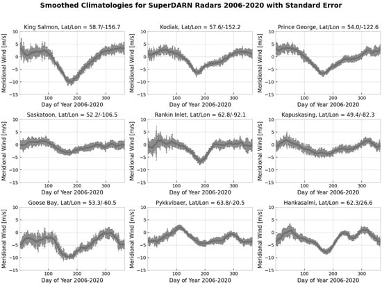
Figure 1.
Radar station climatology data. Smoothed yearly climatology of meridional winds at each of the 9 stations from the years 2006–2020, along with the standard errors (grey brackets).
A recent study [22] reviewed the applications of meteor radar to measure dynamical parameters in the mesosphere/lower thermosphere. A previous study [23] used interferometry to determine that the meteor distribution is nearly Gaussian and centered at 102–103 km, with a full width at a half maximum of approximately 30 km. The radars measure the line-of-sight meteor trail velocities using a number of narrow, approximately 1°-wide beams that typically span a 45° swath. Although vector winds are fitted to the line-of-sight meteor winds measured over the course of an hour, only the meridional component was used in this analysis. This is because with the typical orientation of the radars, one of the beams is aligned in the meridional direction, allowing for greater precision of the meridional component [18]. These winds have been found to correlate best with winds measured by height-resolving meteor radars at 95 km [24,25,26].
2.2. Analysis
The SuperDARN hourly winds underwent quality control to exclude wind values higher than 100 ms−1 or with standard deviations of zero. Additionally, data flagged as due to non-standard operation of the radar were also excluded. Then, the 8, 12, and 24 h tidal wave components and the mean wind values were least-squares-fitted within a 4-day sliding window shifted in one-day increments to remove the tidal components and extract the mean wind values. A 4-day segment was selected for analysis if it passed the quality check [15]. Additionally, 4-day segments that had data gaps >3 h occurring at the same hours each day were excluded. Similarly, 4-day segments with data gaps >12 h that covered the same hours in both halves of the segment were rejected. The 4-day segments were then shifted by 1-day intervals to build up a time series of 4-day running mean winds. Days when these conditions were not met were assigned NaN values.
The daily mean wind climatology was formed by averaging the wind for each day using the 13 years of data and by smoothing the resulting data using a 30-day running mean to remove the effects of any impulsive events [18]. The daily meridional wind anomaly (the daily wind minus the climatology for that day) was then calculated for each station and least-squares-fitted as a sinusoidal function of the station longitude with wavelengths of 360° and 180° to obtain the S1 and S2 waves, respectively. This fit was only performed for the days when a minimum of 5 stations had data available spanning 180°. Individual Hovmöller contour plots of the daily S1 and S2 fitted sine waves as a function of longitude and time were then formed. These formed the basis of the 2D-FFT application, which separated the S1 and S2 waves into eastward- and westward-propagating waves. The latter have been extensively studied using networks of radar observations [17,27,28,29] and models [30] and are not discussed further in this paper. The 2D FFT method was applied over a whole year starting July 1st. The NaN values in the data were interpolated using a third-degree polynomial prior to applying the 2D-FFT, and a Tukey window was used to taper the data to avoid end effects.
As a final step, superposed epoch analysis (SEA) was conducted to better understand the behavior of the EPWs during SSW events. We only considered SSWs followed by an elevated stratopause (hereafter ES-SSWs), which were shown to exert strong influence on the MLT [30]. Using three criteria, including the polar-cap averaged zonal wind and temperature at 1 hPa and the stratopause height to select ES-SSWs events [30], we determined the onset dates of five events over the radar observation period, as listed in Table 1. Note that these criteria differ from the standard World Meteorological Organization (WMO)’s definition of SSW events, which pertains to the 10 hPa level.

Table 1.
The onset dates for the 5 ES-SSWs used in the SEA.
The daily amplitude climatology data of the EPW-S1 and -S2 were first created for each zonal component by excluding those 5 years with an ES-SSW, and therefore, consisted of the remaining 8 years since 2006 and 2020 were not complete years. Each element in the climatology data was formed by obtaining the average of the individual days weighted by their individual fitting variances and included both the standard deviation and the weighted standard error of the mean (SEM). A 61-day smoothing was applied to the climatology data to illustrate the seasonal progression. To perform the SEA, the anomalies for each zonal component were calculated for each year with an ES-SSW event in a window spanning 30 days prior to and 30 days after the onset in that year, with the onset date taken as day zero. The superposed epoch was then created by obtaining the weighted average of each day’s anomaly over the five events, providing the average pre- and post-onset response of the EPWs, as well as the weighted SEM.
3. Results
3.1. Climatology of Meridional Winds at Each Station
The climatology of the meridional wind for each of the nine stations, calculated for the period between 2006 and 2020, is presented in Figure 1. In general, the stations displayed a northward wind in wintertime and an equatorward wind during summer, which started to migrate northward again near the fall equinox. An interesting feature of the climatology data from all nine stations is the large longitudinal difference in the observed summertime meridional wind, as previously reported in SuperDARN data [16]. This strong midsummer equatorward minimum is due to a quasi-stationary PW with a stable year-to-year phase, which results in a bias by adding a longitude-dependent perturbation to the meridional wind. We surmise that that stationary PWs near 95 km may have resulted from gravity wave forcing, which can mirror or “ghost” PW-like features after filtering by the PW-induced winds below [31]. However, this process would mainly apply in winter when PWs are prominent in the stratosphere. As discussed in Section 2, we hereafter subtracted these smoothed climatological meridional winds at each station and retained only the anomalies.
3.2. EPW-S1 and -S2 During Winters Without ES-SSWs
The climatological amplitudes of the EPW-S1 and -S2 were calculated for the 8 years between 2007 and 2019 (Figure 2, top panel), after the removal of the 5 years that featured ES-SSW events during winter (see Section 2). The same climatological data are shown after smoothing using a 61-day boxcar average, as described in Section 2 (Figure 2, bottom panel). From the latter, it is apparent that both the EPW-S1 and -S2 waves gradually built up in amplitude during the winter and reached their maxima in February (3.5 ms−1 around day 230) for S1 and in late January–early February (4 ms−1 around day 210) for S2, before gradually weakening. The red dashed lines show the smoothed climatological data when including all the years. Hence, it appears that the average seasonal evolution was fairly similar in both set of years, except that the wave amplitude for EPW-S1 was slightly higher in January, when the majority of the ES-SSW events during the period investigated occurred (Table 1). This is further examined in the next section. From these climatological, annually varying amplitudes, the EPWs appear to be much more ubiquitous at 95 km than previously assumed, and certainly not strictly limited to periods prior to ES-SSWs. These radar-based observations of meridional winds confirm earlier findings [2] on the ubiquity of EPWs based on re-analyses and MLS satellite observations, albeit here near 95 km (Section 2), i.e., at the upper edge of the layers sampled by MLS.
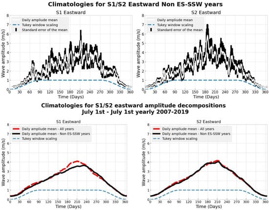
Figure 2.
EPW climatological amplitudes over years without ES-SSWs. Top panel: Climatology of EPW-S1 and -S2 amplitudes in the years without ES-SSWs (white line). The SEM is shown in black. Bottom panel: Climatology in years without ES-SSWs, obtained with a 61-day smoothing of the top panel white curve. The red dashed lines show the smoothed climatological amplitudes in all the years. The blue dashed line shows the Tukey window and how its maximum covers the whole year time scale. Day zero was 1 July.
3.3. EPW-S1 and -S2 During Winters with ES-SSWs
The behaviors of EPW-S1 and -S2 were also examined for years when an ES-SSW happened in the winter. The wave anomalies are presented in Figure 3 and Figure 4 for S1 and S2, respectively, over a 2-month period around each event during individual years and as the average obtained from the SEA (see Section 2). Most of the individual yearly anomalies and the averaged anomalies of EPW-S1 and -S2 show increased peaking within 10 days after the onset (up to 2.5 ms−1 for S1, and up to 1.5 ms−1 for S2 in the SEA). In the pre-onset period, there were also enhancements: the averaged EPW amplitude anomalies display increases of up to 1.5 ms−1 for S1, peaking 22 days before the onset, and of 0.5 ms−1 for S2, peaking about 10 days before the onset. The latter increase in EPW-S2 was not significant, as the SEM only encompasses the zero-amplitude line. However, there was a weak but significant decrease in EPW-S2 in the ten days prior to the onset, which could be indicative of an EPW-S2 critical line descending along with the westward wind layer and blocking it from reaching 95 km. Despite the predominance of the onset dates occurring in the month of January (Table 1), i.e., prior to the EPWs’ climatological seasonal maximum (Figure 2), these rapid enhancements post-onset or pre-onset were faster than the gradual seasonal build-up and may indicate that EPWs are generated from the instability of a disturbed polar vortex.
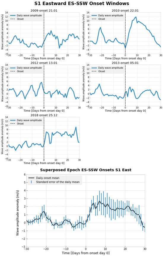
Figure 3.
EPW-S1 in the years with ES-SSWs. Top panel: EPW-S1 amplitudes over 2-month periods around the 5 ES-SSW events. The onset date is indicated for each event. Bottom panel: The mean EPW-S1 amplitude obtained from the SEA based on these five events, centered on the onset date. The blue line indicates the SEM. Raw wind observations carry a measurement error of about 2 ms−1.
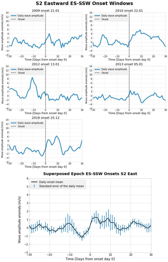
Figure 4.
EPW-S2 in years with ES-SSWs; the same as Figure 3 for EPW-S2.
A closer inspection of individual years indicates that brief enhancements of EPW-S2 prior to the onset occurred without much coherence among the years; the yearly panels reveal large case-to-case variability in their anomalous amplitudes and their timing. A case in point is the January 2012 event, when a clear EPW-S1 post-onset enhancement could not be identified. However, during the same peculiar event (which was not classified as a major warming according to the conventional WMO definition), the pre-onset enhancement of EPW-S2 was the largest among the five cases. This kind of case-to-case variability around the onset time of SSWs has also been discussed in relation to the tidal variability following ES-SSWs [18]. In particular, the winter of 2008/2009 was characterized by a pronounced vortex-split ES-SSW and has been extensively studied in terms of travelling PWs [3,12,30]. During that winter, a weak enhancement of EPW-S2 by 2 ms−1, peaking about 25 days prior to the onset (i.e., in the last days of December 2008) was indeed observed (Figure 5) [12]. EPW-S2 were also observed during other vortex split events [14]. Nevertheless, in our study, the timing of this amplification with respect to the onset was not a robust feature, despite our limited sampling size of five events. A model study [5] also successfully demonstrated the December 2008 S2 enhancement. We now provide model-based results to support the observations from the SuperDARN radar network of a weak but not significant velocity enhancement at 95 km following ES-SSWs.
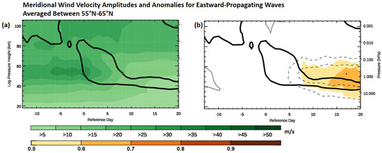
Figure 5.
Model-based composite of ES-SSWs events. (a) Model’s meridional wind velocity amplitudes, and (b) their anomalies, all in 5 m s−1 increments. In (b), positive (negative) anomalies are indicated by solid (dashed) black contours. The probability that the anomaly is abnormal is indicated by orange-shaded contours. In all sub-plots, the zero-wind line is indicated by a thick bold contour. The height–time plots averaged between 55° N and 65° N. The contributions of zonal wavenumbers 1–6 are included.
4. Supporting Model Results
The SuperDARN observations are corroborated by the results from a large-ensemble study comparing 76 ES-SSW periods with 68 wintertime periods without ES-SSWs [5]. This study used version 4 of the Whole Atmosphere Community Climate Model (WACCM), which is a global climate model extending up to ~145 km [32]. An initial model run was performed in the specified dynamics configuration, nudged up to 50 km with 6-hour MERRA-2 horizontal winds and temperature over the period (1980–2013), and with a 10 km linear transition to a free-running layer aloft in the mesosphere and lower thermosphere. This configuration with a nudged troposphere and stratosphere allowed us to model actual ES-SSWs that occurred during the modeled period, ensuring a faithful representation of the events in the stratosphere and troposphere. Four such events were selected from this initial run. These four selected events comprised the two events with onsets in January of 2009 and 2013, which were also included in the current radar-based SEA analysis, and two additional events with onsets in January of 2006 and February 1984. From this initial model run, ensemble members were generated under a similar specified dynamics configuration, but only incorporated a linear transition of nudged MERRA-2 observations from 0 to 0.4 km, essentially leaving the levels above the lowermost troposphere free-running. Ensemble members were initiated by randomly perturbing the temperature field below the model’s rounding error, ~10−14 K, 40 days prior to the four selected ES-SSW onset dates, ultimately simulating 143 wintertime periods, comprising 75 members with ES-SSWs and 68 without. The four sets of ensemble members generated before each ES-SSW event were averaged such that each of the four sets had an equal weight on the results. The ensemble study allowed for a larger sample of ES-SSWs to be composited in SEA than were available from re-analyses alone.
The composited meridional velocity amplitudes and their anomalies in Figure 5a,b showed a slight enhancement of EPW activity in the mesosphere around the onset. At ~95 km, the weak enhancement (up to 5 ms−1 at its peak near day 1) was seen from about 5 days prior to 7 days after onset. Figure 5b shows that, near 95 km, these enhanced amplitudes were not significant, with a probability of less than 0.5 of an amplitude being abnormal. The critical line for EPWs descended alongside the zero-wind line during the ES-SSW onset. This inhibited troposphere-sourced EPWs from propagating into the upper atmosphere after the onset. Figure 5a,b shows a decrease in the EPW amplitude and a significant negative anomaly following the onset.
Additionally, the model allowed us to evaluate simulated winds across a range of altitudes. Near 50 km, the amplitudes of EPWs were markedly suppressed after the ES-SSW onset, with a probability greater than 0.6 of EPW amplitudes being abnormally small.
5. Conclusions
Several studies [2,3,5,33] have pointed out the important role played by EPWs generated from the instability of the background eastward flow. The study by [2] identified a balance between the opposite accelerations provided by the EPW generation and the quasi-stationary PWs’ dissipation in the lower mesosphere, pointing to an essential role of the ubiquitous EPWs in maintaining the zonal momentum balance. Yet, there have been very few studies on the presence of EPWs in the middle atmosphere, and they have been largely based on satellite observations, re-analyses, or model simulations. Most of the studies using observations by ground-based radar networks able to discriminate planetary-scale zonal wavenumbers have been devoted to westward-propagating or quasi-stationary waves [16,17,27,28,29], or to waves with tidal periods [34].
Model studies have suggested that the typical winter mesospheric flow configuration (not subject to SSW events) favors the presence of EPWs in the upper stratosphere and lower mesosphere [3,5]. After an ES-SSW onset, however, a distinctive change in stratospheric wave geometries reduced the EPW amplitude at these altitudes (as shown here in Figure 5), while increasing it above 90 km. However, the wave anomaly above 90 km was not outstanding (statistically significant) compared to non-SSW wintertime conditions.
Our study, based on observations of meridional winds at high northern latitudes by the SuperDARN radar network over the period from 2006 to 2020, indeed indicates that the EPWs are ubiquitous at the observed altitude of around 95 km, as a mean over the latitude belt (49–64° N), with amplitudes up to 6–7 ms−1 and a seasonal peak in January or February, depending on the zonal wavenumber. These findings on the ubiquitous presence of EPWs in an independent dataset confirm a previous satellite-based study [2], although the latter pertained to lower altitudes.
EPWs also appear to be amplified prior to and following ES-SSW onset, but with large event-to-event variability in amplitude and timing. This is corroborated by the composited results from large-ensemble model simulations, which showed slight enhancements of EPW meridional winds in the mesosphere (up to 5 ms−1) from about 5 days prior to 7 days after onset.
The limited impact of EPWs in the stratosphere suggests that their generation in situ, in the MLT, is influential in determining their amplitudes, as opposed to being generated and primed by dynamical conditions in the troposphere.
Author Contributions
Y.J.O. and P.J.E. conceived the project. T.M. carried out the radar data analysis and made the figures as part of her master’s degree in physics at NTNU. C.T.R. contributed with the model simulations. All authors contributed to the overall analysis. The writing was coordinated by Y.J.O. All authors have read and agreed to the published version of the manuscript.
Funding
This research received no external funding.
Institutional Review Board Statement
Not applicable.
Informed Consent Statement
Not applicable.
Data Availability Statement
The SuperDARN data are available from Virginia Tech at http://vt.superdarn.org (accessed 4 November 2024) and from https://superdarn.ca (accessed 4 November 2024). For the results in Section 4, the relevant daily model data can be accessed through the Coastal Carolina University’s Cyber Infrastructure at https://mirror.coastal.edu/sce/CTR_SSWEnsembles (accessed 4 November 2024).
Acknowledgments
The authors acknowledge the use of SuperDARN data. SuperDARN is a collection of radars funded by the national scientific funding agencies of Australia, Canada, China, France, Japan, South Africa, the United Kingdom, and the United States of America. T.M. and P.J.E. also acknowledge W. van Kaspel and E. Vorobeva for helping with the processing of the SuperDARN data.
Conflicts of Interest
The authors declare no conflict of interest.
References
- Domeisen, D.I.V.; Martius, O.; Jiménez-Esteve, B. Rossby wave propagation into the Northern Hemisphere stratosphere: The role of zonal phase speed. Geophys. Res. Lett. 2018, 45, 2064–2071. [Google Scholar] [CrossRef]
- Iwao, K.; Hirooka, T. Opposite contributions of stationary and traveling planetary waves in the northern hemisphere winter middle atmosphere. J. Geophys. Res. Atmos. 2021, 126, e2020JD034195. [Google Scholar] [CrossRef]
- Rhodes, C.T.; Limpasuvan, V.; Orsolini, Y.J. Eastward propagating planetary waves prior to the January 2009 sudden stratospheric warming. J. Geophys. Res. Atmos. 2021, 126, e2020JD033696. [Google Scholar] [CrossRef]
- Harnik, N.; Heifetz, E. Relating overreflection and wave geometry to the counter propagating Rossby wave perspective: Toward a deeper mechanistic understanding of shear instability. J. Atmos. Sci. 2007, 64, 2238–2261. [Google Scholar] [CrossRef]
- Rhodes, C.T.; Limpasuvan, V.; Orsolini, Y.J. The Composite Response of Traveling Planetary Waves in the Middle Atmosphere Surrounding Sudden Stratospheric Warmings through an Overreflection Perspective. J. Atmos. Sci. 2023, 80, 2635–2652. [Google Scholar] [CrossRef]
- Hartmann, D.L. Barotropic instability of the polar night jet stream. J. Atmos. Sci. 1983, 40, 817–835. [Google Scholar] [CrossRef]
- Manney, G.L.; Randel, W.J. Instability at the winter stratopause: A mechanism for the 4-day wave. J. Atmos. Sci. 1993, 50, 3928–3938. [Google Scholar] [CrossRef]
- Orsolini, Y.; Simon, P. Idealized life cycles of planetary-scale barotropic waves in the middle atmosphere. J. Atmos. Sci. 1995, 52, 3817–3835. [Google Scholar] [CrossRef]
- Watanabe, S.; Tomikawa, Y.; Sato, K.; Kawatani, Y.; Miyazaki, K.; Takahashi, M. Simulation of the eastward 4-day wave in the Antarctic winter mesosphere using a gravity wave resolving general circulation model. J. Geophys. Res. Atmos. 2009, 114, D16111. [Google Scholar] [CrossRef]
- Lu, X.; Chu, X.; Fuller-Rowell, T.; Chang, L.; Fong, W.; Yu, Z. Eastward propagating planetary waves with periods of 1-5 days in the winter Antarctic stratosphere as revealed by MERRA and lidar. J. Geophys. Res. Atmos. 2013, 118, 9565–9578. [Google Scholar] [CrossRef]
- Yoo, J.; Chun, H.; Kang, M. Vortex preconditioning of the 2021 sudden stratospheric warming: Barotropic-baroclinic instability associated with the double westerly jets. Atmos. Chem. Phys. 2023, 23, 10869–10881. [Google Scholar] [CrossRef]
- Iida, C.; Hirooka, T.; Eguchi, N. Circulation changes in the stratosphere and mesosphere during the stratospheric sudden warming event in January 2009. J. Geophys. Res. Atmos. 2014, 119, 7104–7115. [Google Scholar] [CrossRef]
- Gelaro, R.; McCarty, W.; Suárez, M.J.; Todling, R.; Molod, A.; Takacs, L.; Randles, C.A.; Darmenov, A.; Bosilovich, M.G.; Reichle, R. The Modern-Era Retrospective Analysis for Research and Applications, version 2 (MERRA-2). J. Clim. 2017, 30, 5419–5454. [Google Scholar] [CrossRef] [PubMed]
- Ma, Z.; Gong, Y.; Zhang, S.; Xiao, Q.; Huang, C.; Huang, K. Quasi–5–day oscillations during Arctic major sudden stratospheric warmings from 2005 to 2021. J. Geophys. Res. Space Phys. 2024, 129, e2023JA032292. [Google Scholar] [CrossRef]
- Kleinknecht, N.H.; Espy, P.J.; Hibbins, R.E. Climatology of zonal wave numbers 1 and 2 planetary wave structure in the MLT using a chain of Northern Hemisphere SuperDARN radars. J. Geophys. Res. Atmos. 2014, 119, 1292–1307. [Google Scholar] [CrossRef]
- Stray, N.H.; de Wit, R.J.; Espy, P.J.; Hibbins, R.E. Observational evidence for temporary planetary-wave forcing of the MLT during fall equinox. Geophys. Res. Lett. 2014, 41, 6281–6288. [Google Scholar] [CrossRef]
- Stray, N.H.; Orsolini, Y.J.; Espy, P.J.; Limpasuvan, V.; Hibbins, R.E. Observations of planetary waves in the mesosphere-lower thermosphere during stratospheric warming events. Atmos. Chem. Phys. 2015, 15, 4997–5005. [Google Scholar] [CrossRef]
- Hibbins, R.E.; Espy, P.J.; Orsolini, Y.J.; Limpasuvan, V.; Barnes, R.J. SuperDARN observations of semidiurnal tidal variability in the MLT and the response to sudden stratospheric warming events. J. Geophys. Res. Atmos. 2019, 124, 4862–4872. [Google Scholar] [CrossRef]
- Greenwald, R.A.; Baker, K.B.; Hutchins, R.A.; Hanuise, C. An HF phase-array radar for studying small-scale structure in the high-latitude ionosphere. Radio Sci. 1985, 20, 63–79. [Google Scholar] [CrossRef]
- Hall, G.E.; MacDougall, J.W.; Moorcroft, D.R.; St.-Maurice, J.P.; Manson, A.H.; Meek, C.E. Super Dual Auroral Radar Network observations of meteor echoes. J. Geophys. Res. 1997, 14, 603–614. [Google Scholar] [CrossRef]
- van Caspel, W.E.; Espy, P.J.; Hibbins, R.E.; McCormack, J.P. Migrating tide climatologies measured by a high-latitude array of SuperDARN HF radars. Ann. Geophys. 2020, 38, 1257–1265. [Google Scholar] [CrossRef]
- Reid, I.M. Meteor Radar for Investigation of the MLT Region: A Review. Atmosphere 2024, 15, 505. [Google Scholar] [CrossRef]
- Chisham, G.; Freeman, M.P. A reassessment of SuperDARN meteor echoes from the upper mesosphere and lower thermosphere. J. Atmos. Sol. Terr. Phys. 2013, 102, 207–221. [Google Scholar] [CrossRef]
- Hibbins, R.E.; Jarvis, M.J. A long-term comparison of wind and tide measurements in the upper mesosphere recorded with an imaging Doppler interferometer and SuperDARN radar at Halley, Antarctica. Atmos. Chem. Phys. 2008, 8, 1367–1376. [Google Scholar] [CrossRef]
- Mitchell, N.J.; Pancheva, D.; Middleton, H.R.; Hagan, M.E. Mean winds and tides in the Arctic mesosphere and lower thermosphere. J. Geophys. Res. 2002, 107, 1004. [Google Scholar] [CrossRef]
- Hussey, G.C.; Meek, C.E.; Andre, D.; Manson, A.H.; Sofko, G.J.; Hall, C.M. A comparison of Northern Hemisphere winds using SuperDARN meteor trail and MF radar wind measurements. J. Geophys. Res. 2000, 105, 18053–18066. [Google Scholar] [CrossRef]
- Koushik, N.; Kumar, K.K.; Ramkumar, G.; Subrahmanyam, K.V.; Kishore Kumar, G.; Hocking, W.K.; He, M.; Latteck, R. Planetary waves in the mesosphere lower thermosphere during stratospheric sudden warming: Observations using a network of meteor radars from high to equatorial latitudes. Clim. Dyn. 2020, 54, 4059–4074. [Google Scholar] [CrossRef]
- Gong, Y.; Li, C.; Ma, Z.; Zhang, S.; Zhou, Q.; Huang, C.; Huang, K.; Li, G.; Ning, B. Study of the quasi-5-day wave in the MLT region by a meteor radar chain. J. Geophys. Res. Atmos. 2018, 123, 9474–9487. [Google Scholar] [CrossRef]
- Ma, Z.; Gong, Y.; Zhang, S.; Zhou, Q.; Huang, C.; Huang, K.; Yu, Y.; Li, G.; Ning, B.; Li, C. Responses of quasi 2day waves in the MLT region to the 2013 SSW revealed by a meteor radar chain. Geophys. Res. Lett. 2017, 44, 9142–9150. [Google Scholar] [CrossRef]
- Limpasuvan, V.; Orsolini, Y.J.; Chandran, A.; Garcia, R.R.; Smith, A.K. On the composite response of the MLT to major sudden stratospheric warming events with elevated stratopause. J. Geophys. Res. Atmos. 2016, 121, 4518–4537. [Google Scholar] [CrossRef]
- Smith, A.K. The origin of stationary planetary waves in the upper mesosphere. J. Atmos. Sci. 2003, 60, 3033–3041. [Google Scholar] [CrossRef]
- Marsh, D.R.; Mills, M.J.; Kinnison, D.E.; Lamarque, J.F.; Calvo, N.; Polvani, L.M. Climate change from 1850 to 2005 simulated in CESM1(WACCM). J. Clim. 2013, 26, 7372–7391. [Google Scholar] [CrossRef]
- Sato, K.; Nomoto, M. Gravity Wave–Induced Anomalous Potential Vorticity Gradient Generating Planetary Waves in the Winter Mesosphere. J. Atmos. Sci. 2015, 72, 3609–3624. [Google Scholar] [CrossRef]
- Yu, Y.; Wan, W.; Ren, Z.; Xiong, B.; Zhang, Y.; Hu, L.; Ning, B.; Liu, L. Seasonal variations of MLT tides revealed by a meteor radar chain based on Hough mode decomposition. J. Geophys. Res. Space Phys. 2015, 120, 7030–7048. [Google Scholar] [CrossRef]
Disclaimer/Publisher’s Note: The statements, opinions and data contained in all publications are solely those of the individual author(s) and contributor(s) and not of MDPI and/or the editor(s). MDPI and/or the editor(s) disclaim responsibility for any injury to people or property resulting from any ideas, methods, instructions or products referred to in the content. |
© 2024 by the authors. Licensee MDPI, Basel, Switzerland. This article is an open access article distributed under the terms and conditions of the Creative Commons Attribution (CC BY) license (https://creativecommons.org/licenses/by/4.0/).