Towards Real-Time Integrated Water Vapor Estimates with Triple-Frequency Galileo Observations and CNES Products

Abstract

Integrated water vapor (IWV) is a crucial parameter for tropospheric sounding and weather prediction applications. IWV is essentially calculated using observations from global navigation satellite systems (GNSS). Presently, the Galileo satellite system is further developed, including more visible satellites that transmit multi-frequency signals. This study aims to evaluate the accuracy of real-time IWV estimated from a triple-frequency Galileo-only precise point positioning (PPP) processing model utilizing E₁, E_5a, E_5b, and E₅ observations, which is not addressed by the previous studies. For this purpose, Galileo datasets from 10 global reference stations spanning various 4-week periods in the winter, spring, summer, and fall seasons are acquired. To process the acquired datasets, dual- and triple-frequency ionosphere-free PPP solutions are used, including E₁E_5a PPP, E₁E_5aE_5b PPP, and E₁E₅E_5b PPP solutions. The publicly available real-time products from the Centre National d’Etudes Spatiales (CNES) are utilized. The real-time IWV values are computed and then validated with the European Centre for Medium-Range Weather Forecasting (ECMWF) reanalysis products (ERA5) counterparts. The findings demonstrate that the root mean square error (RMSE) of the estimated IWV is less than 3.15 kg/m² with respect to the ECMWF ERA5 counterparts. Furthermore, the E₁E_5aE_5b PPP and E₁E₅E_5b PPP models enhance the IWV’s accuracy by about 11% and 16%, respectively, compared with the E₁E_5a PPP model.

1. Introduction

Integrated water vapor (IWV) is the vertically integrated total amount of water vapor in an air column. IWV has large temporal variations depending on the hour, day, month, and season, and it also has spatial variations based on geographic location; additionally, IWV is a key parameter for atmospheric sounding and weather monitoring applications. IWV can be calculated using different techniques, including ground-based and satellite-based techniques. The microwave radiometers, radiosondes, and global navigation satellite systems (GNSS) are the widely used ground-based IWV estimation techniques [1,2,3], particularly the GNSS technique because it has high temporal and spatial resolutions. For satellite-based techniques, the remote sensing satellites with various spectral bands and algorithms are used.

A number of researchers have recently examined the GNSS-derived integrated water vapor’s accuracy, e.g., [4,5,6,7,8,9,10,11,12]. Marut et al. [8] used a local network of low-cost multi-GNSS receivers in order to evaluate the IWV accuracy; in addition, the IWV values have been computed in both real-time and post-processing domains. The obtained IWV values have been compared with the numerical weather model (NWM) and water vapor radiometer (WVR). It has been shown that the standard deviation of the estimated IWV was 5.4 and 1.0 kg/m² in comparison with the NWM and WVR, respectively. The precision of the estimated IWV from a regional network of geodetic GNSS receivers has also been examined in near real-time domains [4]. It has been found that the obtained IWV had good agreement with the European Centre for Medium-Range Weather Forecasting (ECMWF) reanalysis products (ERA5) and atmospheric infrared sounder (AIRS) counterparts.

The GNSS-based integrated water vapor is computed in post-processing or near real-time (NRT) domains. This is due to the 13-day or 6-hour latencies of the IGS final or ultra-rapid products, respectively; therefore, the main challenge for GNSS meteorology applications is to determine the IWV in real-time domains, particularly for nowcasting and short-term severe weather monitoring applications. At present, an accurate real-time precise point positioning (RT-PPP) solution is obtained by using the international GNSS service (IGS) real-time service (RTS) products. Various IGS centers provide the RTS precise satellite orbit and clock correction products; for instance, the Centre National d’Etudes Spatiales (CNES), Bundesamt für Kartographie und Geodäsie (BKG), Geo Forschungs Zentrum (GFZ), IGS, GNSS Research Center of Wuhan University (WHU), Natural Resources Canada (NRCan), and the European Space Agency (ESA). The CNES offers post-processing and real-time products for multi-constellation GNSS users; furthermore, the CNES real-time products have been used in different applications, including PPP [13], PPP-ambiguity resolution [14], tropospheric delay estimation [15], and ionospheric delay mitigation [16].

From the aforementioned studies, it can be seen that the IWV has been estimated using dual-frequency GPS or dual-frequency multi-GNSS PPP solutions (i.e., GPS plus other constellations) in post-processed mode; however, the previous studies did not address the retrieval of the IWV in real-time mode with real-time products, using a single-constellation GNSS system away from GPS or utilizing triple-frequency observations. Consequently, the main motivation of this study is to use a triple-frequency Galileo-only PPP solution benefiting from multi-frequency observations, which are transmitted by all Galileo satellites other than GPS that are only available for a number of GPS satellites. Adding triple-frequency observations to the IWV estimation scenario means that measurement redundancy and various linear-combinations can be formed; hence, the aim is to develop different ionosphere-free Galileo PPP models, including dual- and triple-frequency solutions (i.e., E₁E_5a PPP, E₁E_5aE_5b PPP, and E₁E₅E_5b PPP) to estimate the IWV values. The IWV is estimated in real-time domains utilizing the CNES real-time satellite orbit and clock products; additionally, the real-time IWV’s spatiotemporal variability is further investigated because it is a crucial parameter for weather and climate applications. The ECMWF ERA5 IWV counterparts are used as references for the obtained IWV findings.

2. Galileo PPP Processing Models

The basic formulas for Galileo pseudo-range and carrier phase observations can be expressed mathematically as follows [17]:

$$P_i^E={\rho }_r^E+c\left({dt}_r{-dt}^E\right)+I_{r,i}^E+T_r^E+c\left(B_{r,i}-B_i^E\right)+{\epsilon }_{P,i}$$

(1)

$${\mathsf{\Phi }}_i^E={\rho }_r^E+c\left({dt}_r{-dt}^E\right)-I_{r,i}^E+T_r^E+c\left({\delta }_{r,i}-{\delta }_i^E\right)+{\lambda }_i{N}_{r,i}^E+{\epsilon }_{\Phi ,i}$$

(2)

where $i$, $E,$ and $r$ denote to frequency, Galileo system, and receiver, respectively; $P$ and $\mathsf{\Phi }$ refer to pseudo-range and carrier phase observations, respectively; ${\rho }_r^E$ denotes the true geometric range between the satellite and receiver; $c$ is the light’s speed in a vacuum; ${dt}_r$ and ${dt}^E$ are the clock errors related to the receiver and satellite, respectively; $I_{r,i}^E$ and $T_r^E$ refer to ionospheric and tropospheric delay, respectively; $B_{r,i}$ and $B_i^E$ are the receiver and satellite code hardware delay, respectively; ${\delta }_{r,i}$ and ${\delta }_i^E$ are the receiver and satellite phase hardware delay, respectively; ${\lambda }_i$ indicates the wavelength of the carrier phase measurement; $N_{r,i}^E$ is the non-integer ambiguity parameter; and ${\epsilon }_{P,i}$ and ${\epsilon }_{\Phi ,i}$ are the un-modeled residual errors for both the code and carrier phase measurements, respectively.

2.1. Dual-Frequency Ionosphere-Free Galileo PPP Model

Using both code and carrier phase observations, the dual-frequency ionosphere-free E₁/E_5a Galileo PPP mathematical model can be formulated as follows [17]:

$$P_{IF}={\rho }_r^E+c\left({dt}_r{-dt}^E\right)+T_r^E+c\left(∆B_r-{\mathsf{\Delta }B}^E\right)+{\epsilon }_{P,IF}$$

(3)

$${\mathsf{\Phi }}_{IF}={\rho }_r^E+c\left({dt}_r{-dt}^E\right)+T_r^E+c\left({\mathsf{\Delta }\delta }_r-\mathsf{\Delta }{\delta }^E\right)+\overline{\lambda N_r^E}+{\epsilon }_{\Phi ,IF}$$

(4)

where $P_{IF}$ and ${\mathsf{\Phi }}_{IF}$ denote the ionosphere-free linear combination of dual-frequency code and carrier phase observations, respectively; $\mathsf{\Delta }{B}_r$ and ${\mathsf{\Delta }B}^E$ are the receiver and satellite ionosphere-free differential code bias (DCB), respectively; ${\mathsf{\Delta }\delta }_r$ and $\mathsf{\Delta }{\delta }^E$ are the receiver and satellite ionosphere-free differential phase bias (DPB), respectively; and $\overline{\lambda N_r^E}$ indicates the ionosphere-free ambiguity term for the carrier phase measurements.

The differential code biases are mainly lumped into both receiver and satellite clock errors for the dual-frequency Galileo PPP model, as given below:

$$P_{IF}={\rho }_r^E+c\left({dt}_r+{\mathsf{\Delta }B}_r\right)-c\left({ dt}^E+{\mathsf{\Delta }B}^E\right)+T_r^E+{\epsilon }_{P,3}$$

(5)

$${\mathsf{\Phi }}_{IF}={\rho }_r^E+c\left({dt}_r+{\mathsf{\Delta }B}_r\right)-c\left({ dt}^E+{\mathsf{\Delta }B}^E\right)+T_r^E+\left(\overline{\lambda N_r^E}+D_r-D^E\right)+{\epsilon }_{\Phi ,IF}$$

(6)

where $D_r$ indicates the difference between the DCB and DPB for the receiver, and $D^E$ denotes the difference between the DCB and DPB for the satellite. The PPP model can be reformulated using the precise satellite clock products, as shown below:

$$P_{IF}={\rho }_r^E+c{dt}_r^{~}-c{dt}_p^E+T_r^E+{\epsilon }_{P,3}$$

(7)

$${\mathsf{\Phi }}_{IF}={\rho }_r^E+c{dt}_r^{~}-c{dt}_p^E+T_r^E+\left(\overline{\lambda N_r^E}+D_r-D^E\right)+{\epsilon }_{\Phi ,IF}$$

(8)

where ${dt}_r^{~}$ is the receiver DCB plus the receiver clock parameter, and ${dt}_p^E$ indicates the Galileo precise satellite clock parameter.

2.2. Triple-Frequency Ionosphere-Free Galileo PPP Model

To form the triple-frequency ionosphere-free Galileo PPP processing model, two dual-frequency ionosphere-free linear combinations are used for both the code and phase measurements, as follows [18]:

$$P_{IF,12}={\rho }_r^E+c{dt}_{r,12}-c{dt}_{p,12}^E+c{\mathsf{\Delta }B}_{r,12}+c{\mathsf{\Delta }B}_{12}^E+T_r^E+{\epsilon }_{P,12}$$

(9)

$$P_{IF,13}{=\rho }_r^E+c{dt}_{r,12}-c{dt}_{p,12}^E-c{\mathsf{\Delta }B}_{13}^E+T_r^E+IFB+{\epsilon }_{P,13}$$

(10)

$${\mathsf{\Phi }}_{IF,12}={\rho }_r^E+c{dt}_{r,12}-c{dt}_{p,12}^E+T_r^E+\left(\overline{\lambda N_{r,12}^E}+D_{r,12}-D_{12}^E\right)+{\epsilon }_{\Phi ,12}$$

(11)

$${\mathsf{\Phi }}_{IF,13}={\rho }_r^E+c{dt}_{r,12}-c{dt}_{p,12}^E+T_r^E+\left(\overline{\lambda N_{r,13}^E}+D_{r,13}-D_{13}^E+IFB\right)+{\epsilon }_{\Phi ,13}$$

(12)

where $P_{IF,12}$ and ${\mathsf{\Phi }}_{IF,12}$ denote the E₁E_5a or E₁E₅ ionosphere-free combination of code and phase measurements, respectively; $P_{IF,13}$ and ${\mathsf{\Phi }}_{IF,13}$ refer to the E₁/E_5b ionosphere-free combination of code and phase measurements, respectively; and $IFB$ indicates the inter-frequency bias (IFB).

It can be noticed that both satellite and receiver clocks are determined for the E₁/E_5a combination; moreover, the DCBs are not lumped into satellite and receiver clocks. This is attributed to the fact that there are various DCBs on each ionosphere-free linear combination; as a result, an inter-frequency bias parameter is presented in the E₁/E_5b linear combination. Inter-frequency bias is the difference between the ionosphere-free receiver DCB12 and DCB13 ($IFB={\mathsf{\Delta }B}_{r,12}-{\mathsf{\Delta }B}_{r,13}$). The IFB is lumped into the ambiguity term for carrier phase measurements.

3. Integrated Water Vapor Computation

The tropospheric delay ($T_r^E$) is broken down into two components, the hydrostatic delay and the wet delay, as shown below:

$$T_r^E={{{m_h^{E}Z}_h+m}_w^{E}Z}_w$$

(13)

where $m_h^E$ and $m_w^E$ refer to the mapping functions for the hydrostatic and wet parts, respectively, and $Z_h$ and $Z_w$ are the zenith hydrostatic delay (ZHD) and zenith wet delay (ZWD), respectively. In this study, the Saastamoinen model [19] is used in order to compute the ZHD with surface meteorological parameters estimated from the global pressure and temperature 2 wet (GPT2w) model [20]; furthermore, Vienna mapping functions 1 (VMF1) [21] for both hydrostatic and wet parts are used. In addition, the ZWD is determined as an unknown parameter in the processing model.

Once the ZWD is computed, the IWV can be calculated using the following formula [17]:

$$IWV={10}^6{\left[{ \rho }_w{R}_w\left({\displaystyle \frac{k_3}{T_m}}+k_2^{\prime }\right)\right]}^{-1}\times Z_w$$

(14)

where ${ \rho }_w$ refers to the liquid water density (${\rho }_w$ = 997 kg/m³); $R_w$ indicates the water vapor’s gas constant ($R_w$ = 461.525 J/K.Kg); $k_3$ is the troposphere refractivity coefficient ($k_3$ = 3754.63 K²/Pa); $T_m$ denotes the weighted mean temperature (K), which is calculated based on the surface temperature ($T_s$) at the reference station ($T_m=70.2+0.72T_s$) [17]; and $k_2^{\prime }$ is also a tropospheric refraction coefficient, and it is determined using the following equation:

$$k_2^{\prime }=k_2-\left(k_1{\displaystyle \frac{M_w}{M_d}}\right)$$

(15)

where $k_1$ and $k_2$ are coefficients ($k_1$ = 0.776890 K/Pa and $k_2$ = 0.712952 K/Pa); $M_w$ refers to the wet air’s molar mass ($M_w$ = 15.9994 g/mol); and $M_d$ is the dry air’s molar mass ($M_d$ = 28.9644 g/mol).

4. Processing of Galileo Datasets

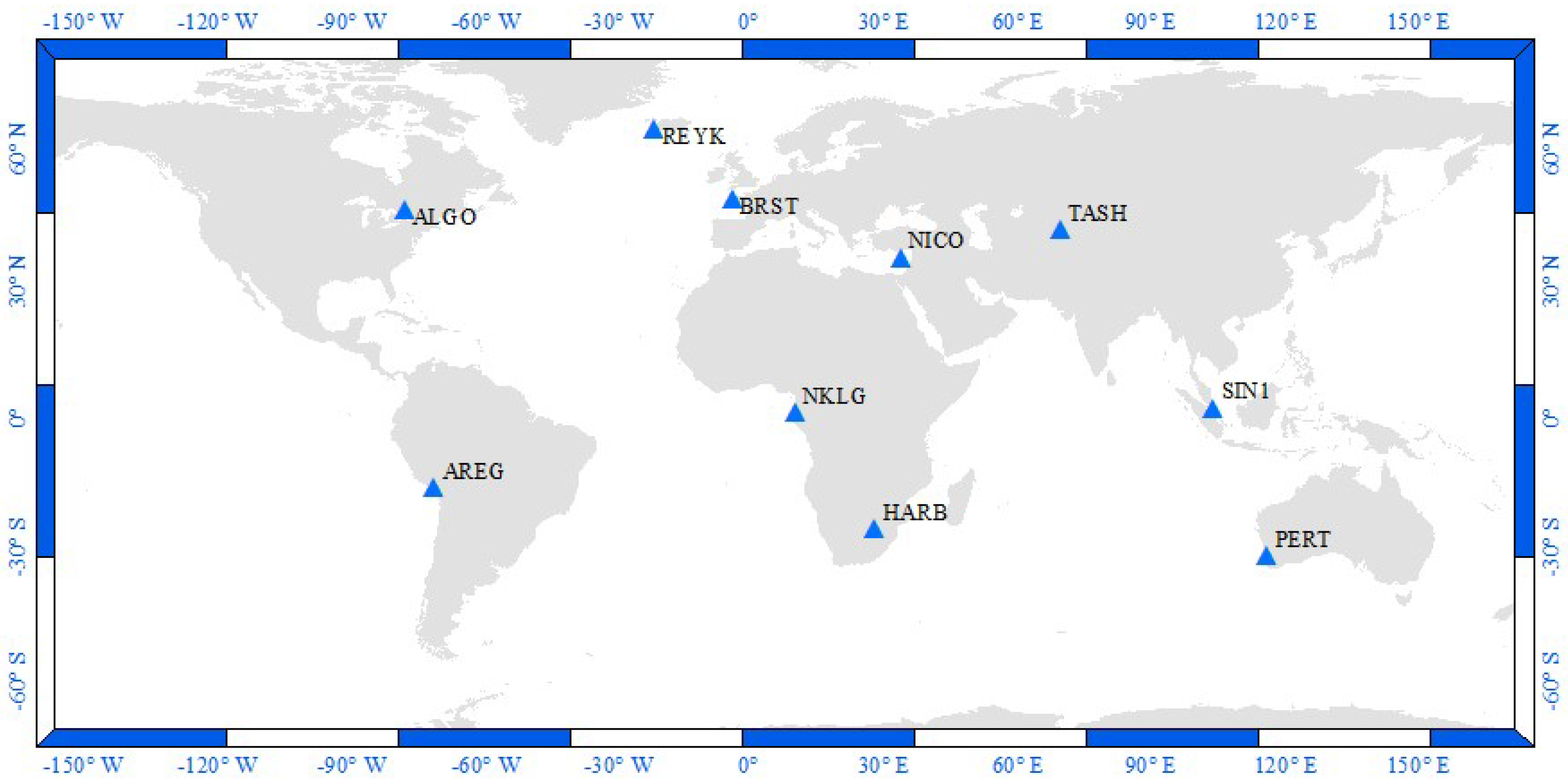
RINEX 3.03 Galileo datasets from 10 globally distributed IGS stations have been downloaded (Figure 1) in order to assess the precision of the computed real-time IWV. To examine different tropospheric properties, stations have been chosen from various longitudes, latitudes, and heights, as given in

Table 1. Reference stations’ coordinates.

Station	Longitude	Latitude	Height	Station	Longitude	Latitude	Height
REYK	338.045	64.139	93.0	SIN1	103.679	1.34297	92.9
BRST	355.503	48.381	65.8	NKLG	9.672	0.353	31.5
ALGO	281.929	45.956	201.0	AREG	288.507	−16.465	2489.4
TASH	69.296	41.328	437.9	HARB	27.707	−25.887	1558.1
NICO	33.396	35.141	190.0	PERT	115.885	−31.802	12.7

. Static triple-frequency Galileo measurements spanning 24 h over a period of four different weeks have been used [22]. The four weeks have been selected to be within the day of year (DOY) 24–30, 101–107, 192–198, and 290–296 in the year 2021, which represent the winter, spring, summer, and autumn seasons, respectively; additionally, the hourly, daily, and seasonal variations of the estimated real-time IWV have been investigated.

Various triple-frequency ionosphere-free (IF) Galileo precise point positioning models have been used, which are E₁E_5aE_5b PPP and E₁E₅E_5b PPP, to process the observation datasets. The E₁E_5aE_5b PPP processing model is a combination of IF_E1E5a +IF_E1E5b, while the E₁E₅E_5b PPP processing model is IF_E1E5 +IF_E1E5b. The dual-frequency ionosphere-free E₁E_5a PPP Galileo PPP solution is used as well.

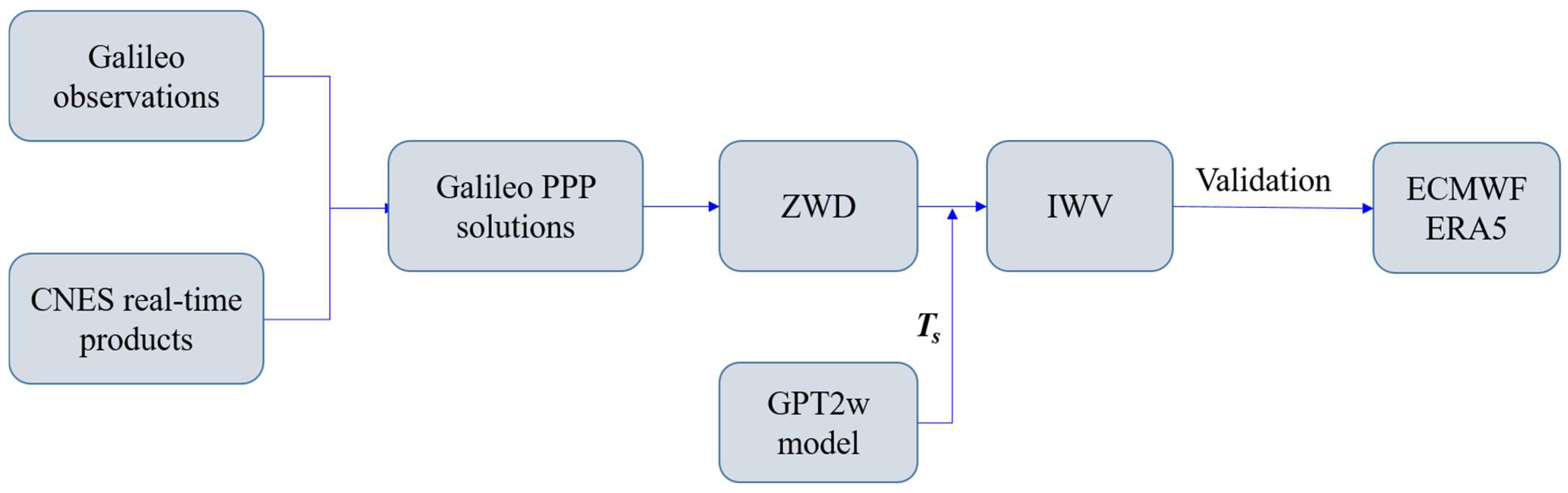
For the proposed Galileo PPP solutions, the real-time satellite clock and orbit products available from the CNES [23] have been utilized to correct the satellite clock and orbit errors; moreover, CNES real-time code biases products have been used to ensure that pseudo-range measurements had consistency with satellite clock products. For tropospheric parameters estimation, the Saastamoinen tropospheric model has been used in order to calculate the zenith hydrostatic delay, and the Vienna mapping function for both hydrostatic and wet parts has been utilized as well. The processing parameters have been estimated using the least squares algorithm. To process our datasets, the Net_Diff GNSS software [24] has been used.

Thereafter, the estimated integrated water vapor values are compared and validated with the obtained IWV through the ECMWF reanalysis products [25]. For the ECMWF integrated water vapor estimation, GNSS observations are collected from both the IGS and European permanent network (EPN) reference stations; then, the datasets are processed to obtain the ZTD values. The IWV can be determined using the estimated ZTD along with the surface metrological parameters. There are two types of integrated water vapor products with 1 h temporal resolution, which are the estimated IWV from GNSS measurements and the retrieved IWV from ERA5 at the station coordinates, altitude, date, and time products. Both IWV products are computed from the GNSS receiver position to the top of the atmosphere. It should be mentioned that the IWV ERA5 products are used as reference in this research. Moreover, in the IWV calculation (i.e., Equation (14)), to compute the weighted mean temperature ($T_m$), the surface temperature ($T_s$) is extracted from the GPT2w model because the examined stations are not equipped with metrological sensors. Figure 2 summarizes the estimation and validation procedure of the IWV.

5. Analysis of Results

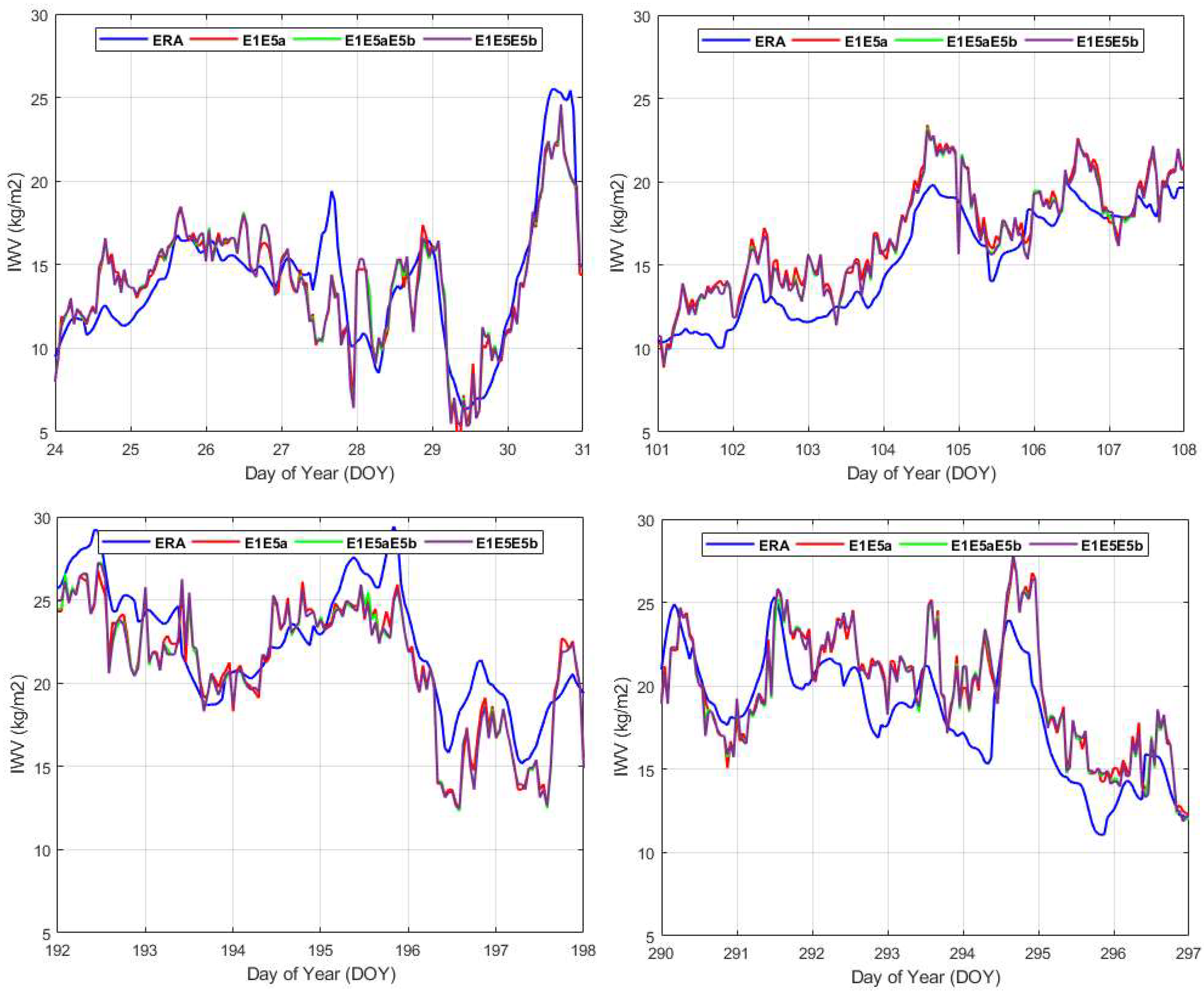
To obtain the IWV values, different Galileo ionosphere-free real-time PPP scenarios are applied including E₁E_5aE_5b PPP, E₁E₅E_5b PPP, and E₁E_5a PPP solutions. The IWV determination is based on the ZWD, which is basically a by-product of the three developed PPP models; subsequently, the computed IWV values are compared with the ECMWF ERA5 IWV counterparts. The real-time IWV are estimated every 1 h over four weeks, representing various seasons to evaluate the estimated real-time IWV performance in hour, day, and season domains.

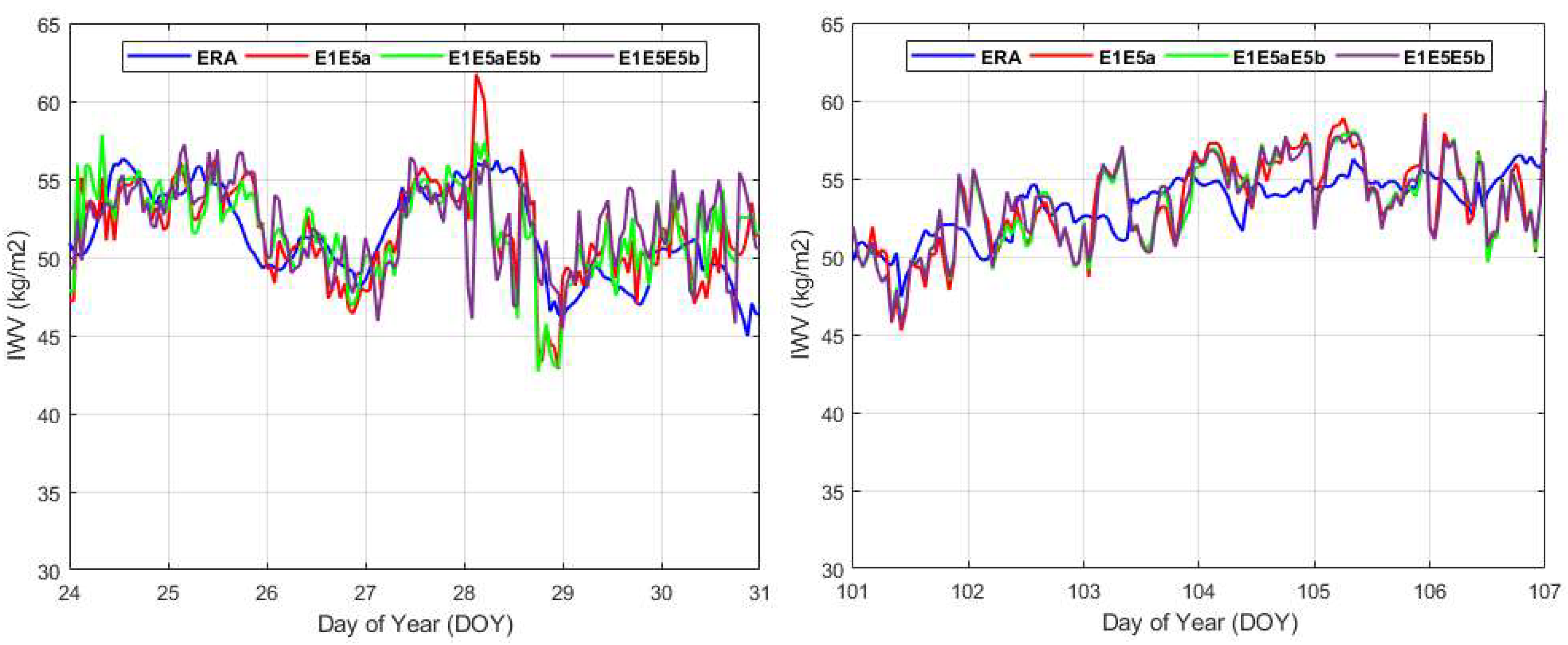
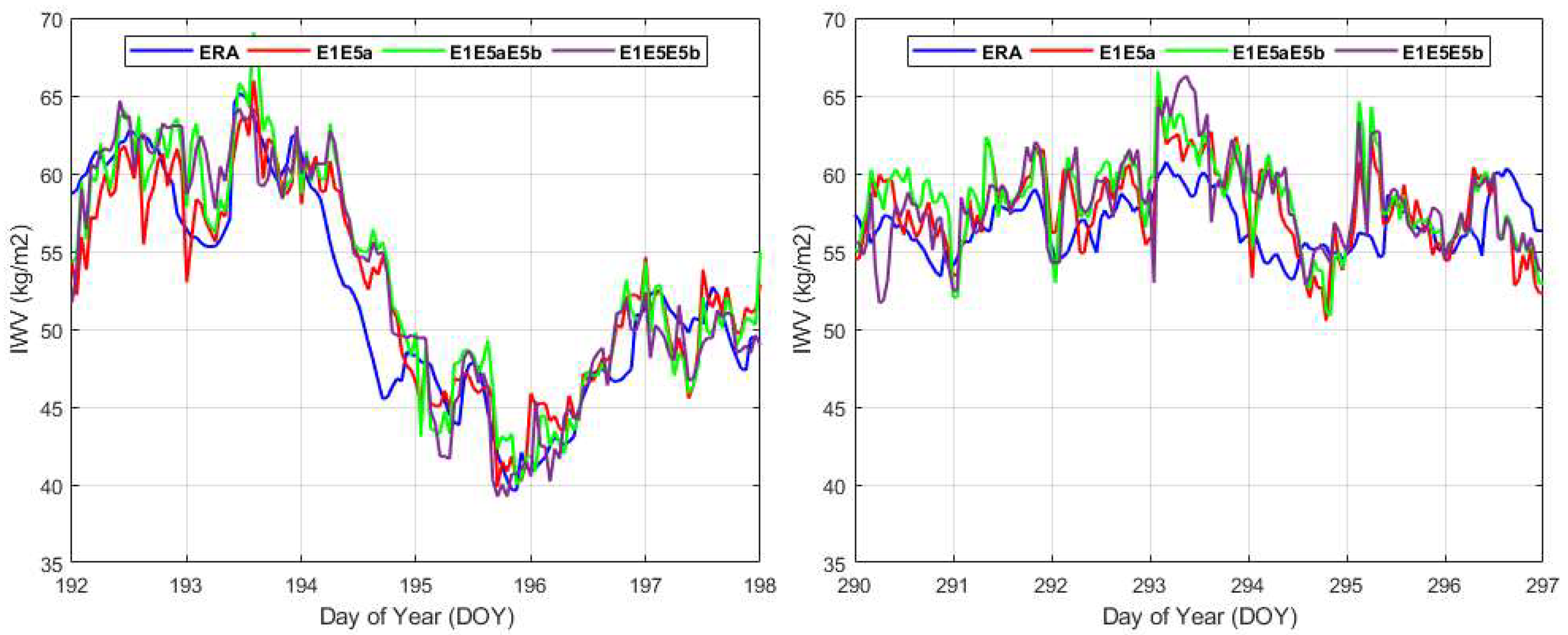
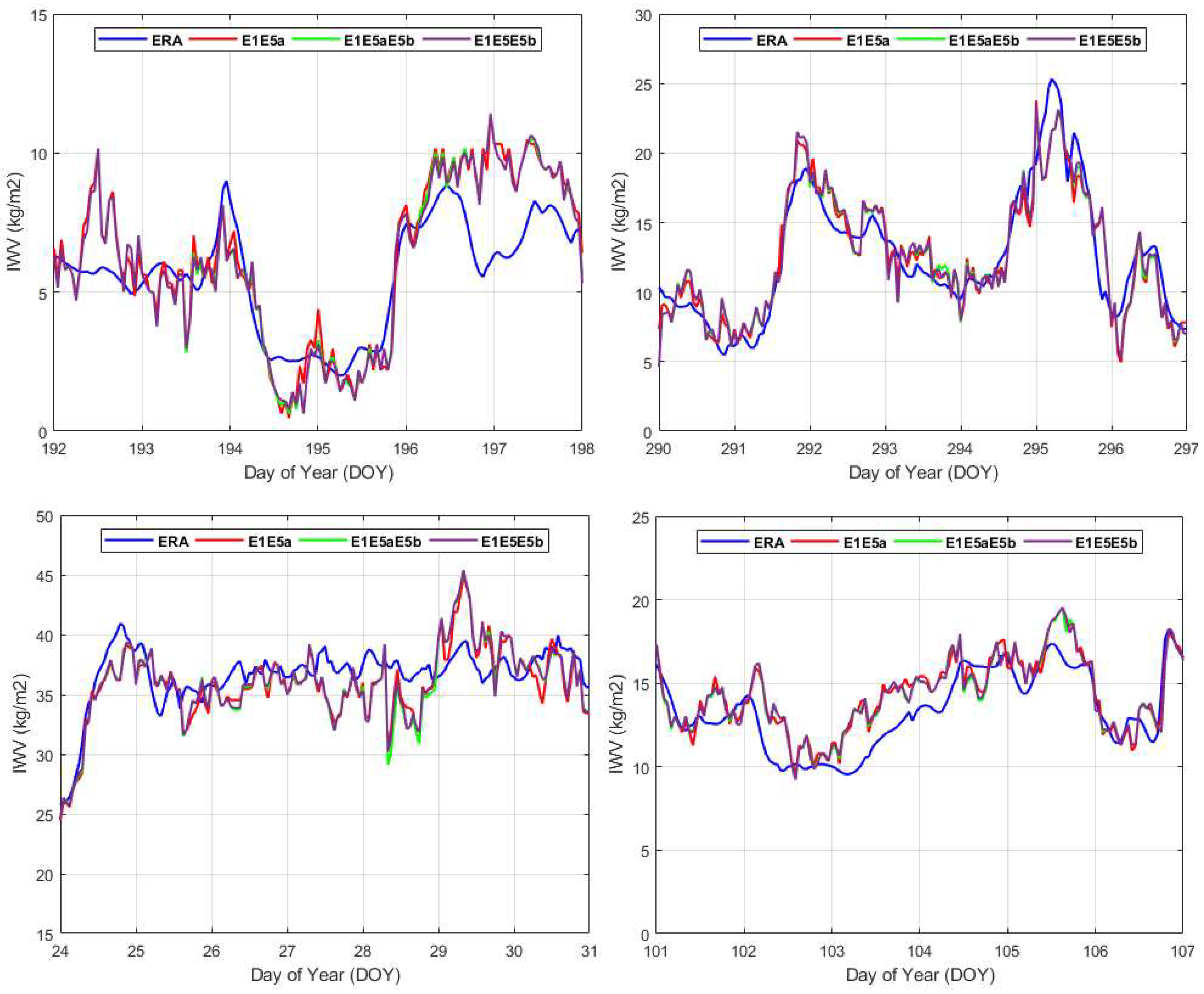
Figure 3, Figure 4 and Figure 5 present the estimated real-time integrated water vapor values from the three Galileo PPP solutions and the ERA5 at stations NICO, SIN1, and HARB, respectively, as examples, over the four selected weeks. It is noticed that the calculated IWV values have agreement with the ERA5 IWVs counterparts; in addition, the estimated integrated water vapors show obvious hourly and daily variations, which is attributed to the fact that the water vapor is a time-dependent parameter. Moreover, station SIN1 has large IWVs compared to the others. This is due to its location, which is in the equatorial zone. For the IWV seasonal variation at station NICO, it is shown that the IWVs in spring and fall are relatively similar; on the other hand, the IWVs reach their maximum and minimum values in summer and winter, respectively. This is attributed to the surface temperature variability in the summer and winter seasons. For station SIN1, the integrated water vapor values are slightly similar in the four seasons, except for the period from DOY 195 to DOY 197. This might be attributed to the decrement of the surface temperature parameter in this period; on the contrary, the seasonal variation of the IWVs at station HARB is obvious. This can be attributed to station HARB’s higher altitude and differences in the surface meteorological parameters as well.

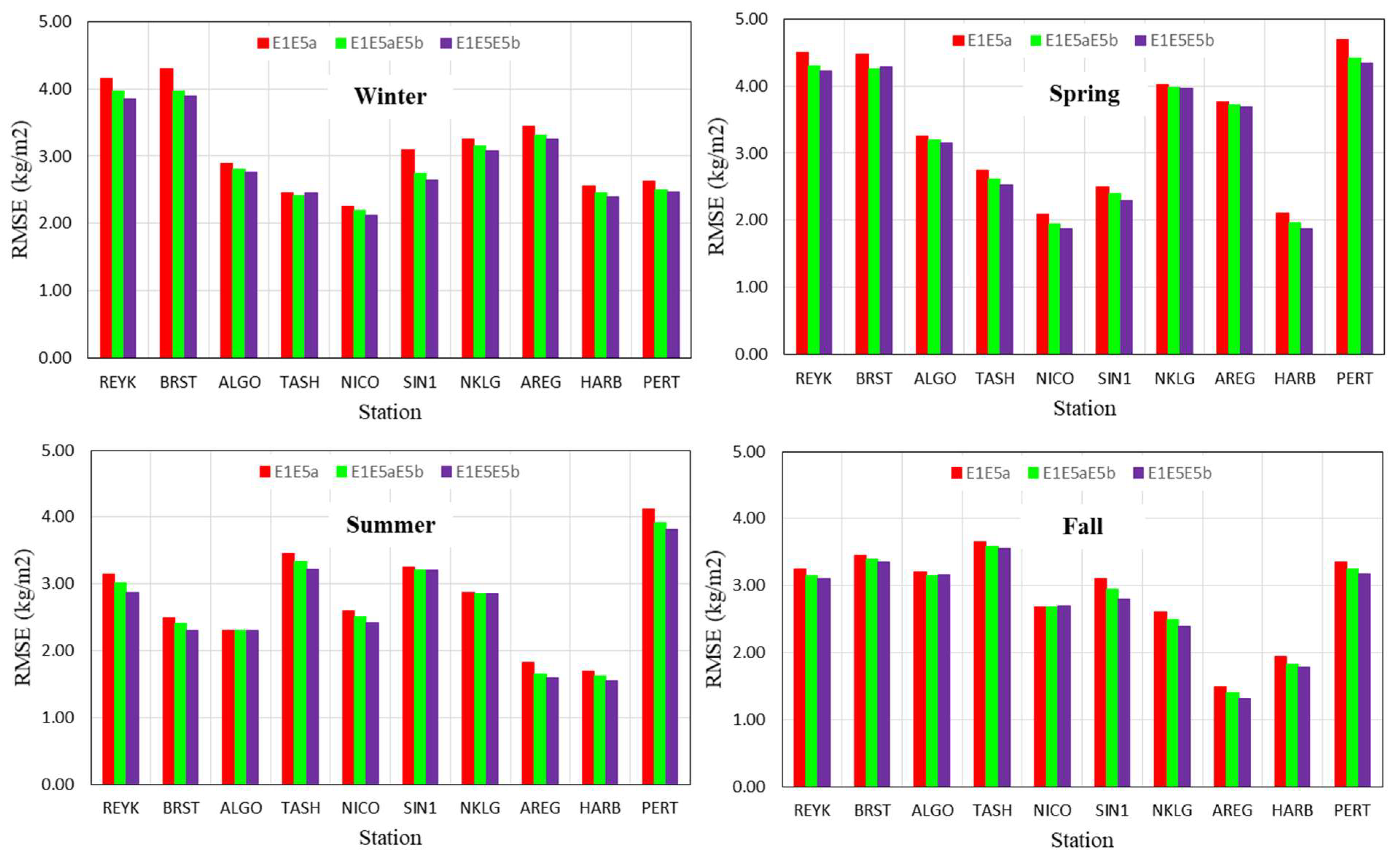
The computed real-time IWVs are validated with the ECMWF ERA5 IWVs through the calculation of the root mean square error (RMSE) for the differences for each station; hence, Figure 6 illustrates the RMSEs for the selected stations in the four seasons. It is shown that the obtained real-time IWVs from the developed Galileo PPP processing models show agreement with the ERA5 counterparts with RMSEs less than 4.2 kg/m²; furthermore, there are slight small differences between the triple-frequency PPP models and the dual-frequency PPP model.

Also, the IWV values show season dependency; for example, stations TASH and NICO have IWV discrepancies in the four seasons; additionally, station REYK has large RMSE values. This may be due to station’s location in a high latitude region. Station PERT also has large RMSEs, which might be attributed to surface temperature variations in the four seasons. The impact of the station’s altitude on the IWV values and their variations is obvious for stations AREG and HARB. The RMSE values are slightly similar in the four seasons for stations SIN1 and NKLG because these stations are located in the equatorial region, in which the surface meteorological parameters are relatively similar in the four seasons.

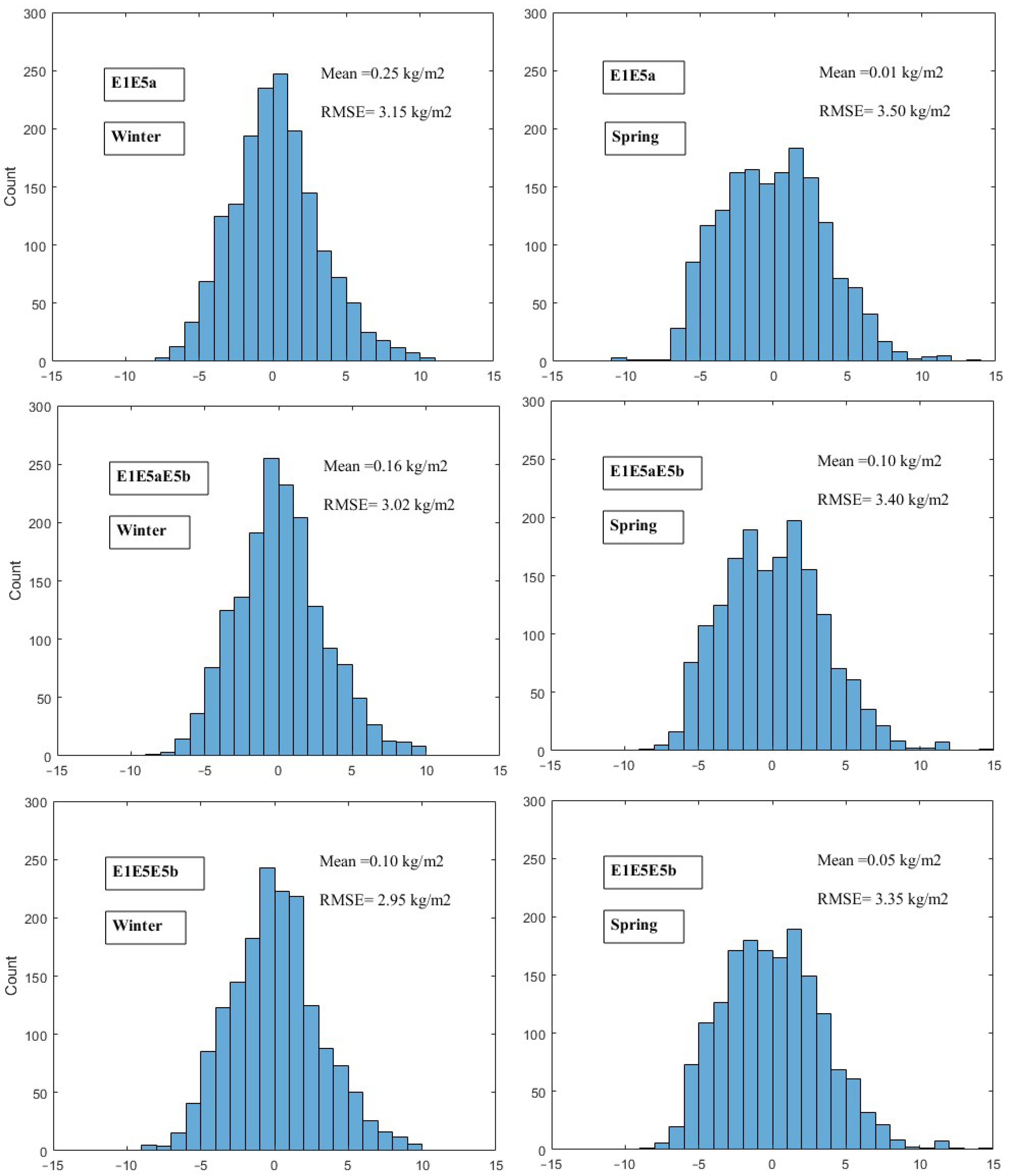
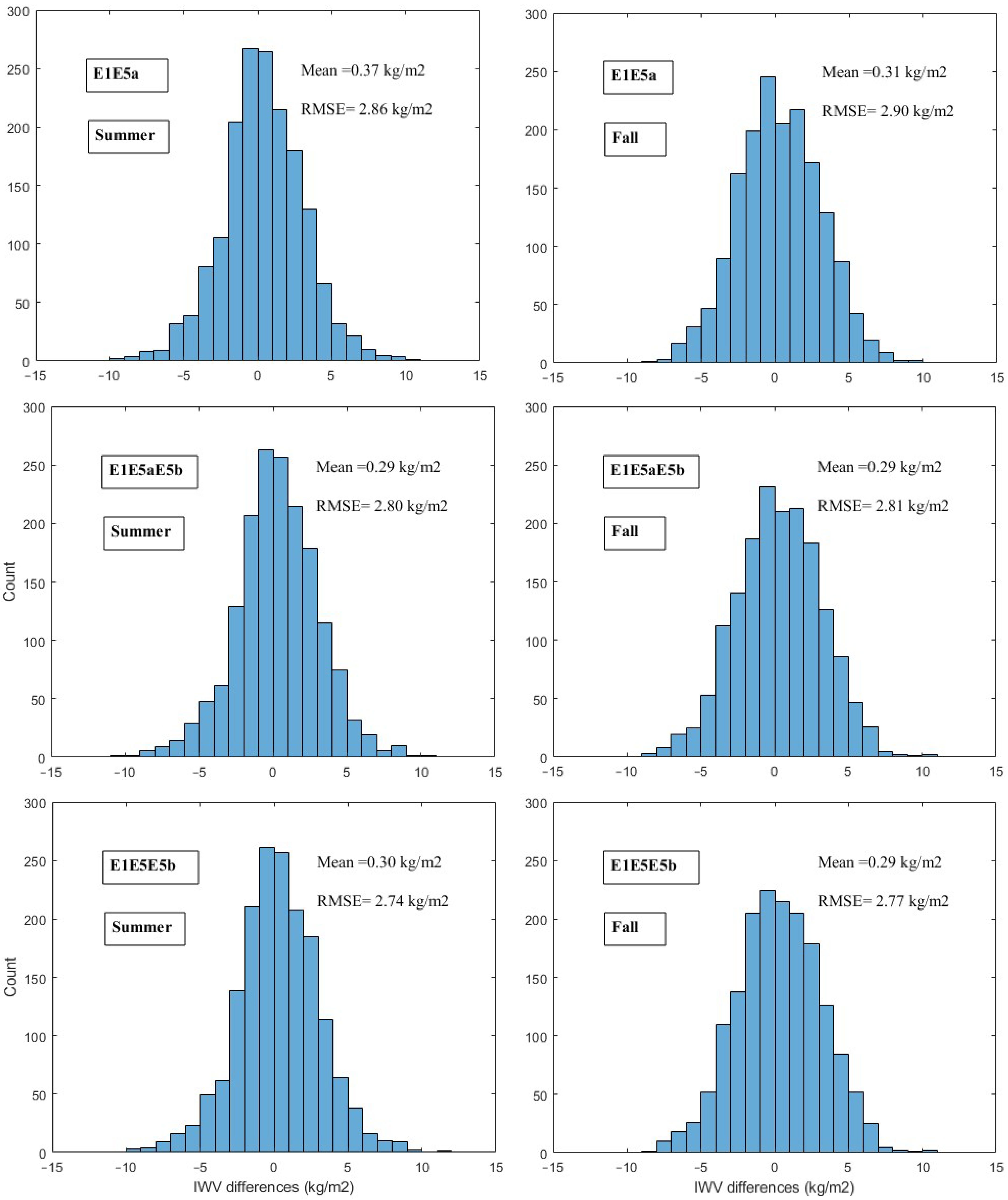
To further assess the computed integrated water vapor accuracy in different seasons, the distribution of the IWV differences are computed, as presented in Figure 7. The mean and RMSE of the differences are calculated as well. It is clear that the estimated IWVs are close to the ERA5 counterparts in the four seasons with RMSEs less than 3.5 kg/m²; in addition, the accuracy of the IWV is further enhanced when the third-frequency Galileo measurements are added to the PPP processing model. The RMSE is enhanced in winter from 3.15 to 3.02 kg/m² and from 3.15 to 2.95 kg/m² for the E₁E_5aE_5b PPP and E₁E₅E_5b PPP models, respectively, in comparison with the E₁E_5a PPP model. Moreover, the estimated IWVs accuracy is enhanced in spring from 3.5 to 3.40 and 3.35 kg/m² for the E₁E_5aE_5b PPP and E₁E₅E_5b PPP processing models, respectively; furthermore, in summer, the RMSE values decreased from 2.86 to 2.80 and 2.74 kg/m² when the E₁E_5aE_5b PPP and E₁E₅E_5b PPP models are used, respectively. In the fall season, the E₁E_5aE_5b PPP and E₁E₅E_5b PPP models also reduce the IWV error from 2.90 to 2.81 and 2.77 kg/m² with respect to the dual-frequency PPP model.

The overall accuracy of the IWV is further investigated through determination of the mean, minimum, maximum, and RMSE parameters (

Table 2. Statistical analysis for the obtained IWVs.

Solution	Statistical Parameters (kg/m2)
	Mean	Minimum	Maximum	RMSE
E1/E5a PPP	0.24	−10.76	14.65	3.15
E1/E5a/E5b PPP	0.21	−10.09	13.69	2.80
E1/E5/E5b PPP	0.18	−9.61	13.01	2.65

); it is found that the accuracy of the estimated IWVs from the E₁E_5aE_5b PPP model is improved by about 11% in comparison with those computed from the E₁E_5a PPP model. Moreover, improvement in IWVs estimation by about 16% is obtained through the E₁E₅E_5b PPP processing model with respect to the E1E5a PPP processing model.

Generally, based on the obtained results, it can be said that the integrated water vapor shows hourly, daily, seasonal, and spatial dependency; furthermore, the obtained real-time IWVs from the proposed PPP models show agreement with respect to the ECMWF ERA5 counterparts with RMSE values less than 3.15 kg/m². The estimated IWVs from the triple-frequency Galileo PPP model are more accurate than those from the dual-frequency Galileo PPP model. This is attributed to measurement redundancy. Furthermore, the E₁E₅E_5b PPP model slightly improves the IWV accuracy compared to the E₁E_5aE_5b PPP model. This may be due to the quality of the observations.

6. Conclusions

In this research, a real-time integrated water vapor computation method based on the Galileo PPP processing model and real-time CNES products has been proposed. Galileo observations (i.e., E₁, E_5a, E_5b, and E₅) from a number of global reference stations over a period of four different weeks have been utilized to examine the IWV’s hourly, daily, seasonal, and spatial variations. The datasets have been processed using various processing scenarios, which are Galileo E₁E_5a PPP (i.e., by combining E₁ and E_5a observations), E₁E_5aE_5b PPP (i.e., by combining E₁, E_5a, and E_5b observations), and E₁E₅E_5b PPP (i.e., by combining E₁, E₅, and E_5b observations) models. The resulted integrated water vapor values have been validated with the ECMWF ERA5 counterparts. It has been shown that the Galileo-derived IWV values had good agreement with the ERA5 counterparts with RMSEs less than 3.15 kg/m². Additionally, the E₁E_5aE_5b PPP and E₁E₅E_5b PPP models had superiority to the E₁E_5a PPP model in the IWV calculation. Compared with the E₁E_5a PPP model, the IWV accuracy has been improved by about 11% and 16% for the E₁E_5aE_5b PPP and E1E5E5b PPP models, respectively. According to the obtained findings, these proposed real-time IWV estimation models can be employed in short-term weather predication and atmospheric sounding applications.