A Branched Convolutional Neural Network for Forecasting the Occurrence of Hazes in Paris Using Meteorological Maps with Different Characteristic Spatial Scales

Abstract

A convolutional neural network (CNN) has been developed to forecast the occurrence of low-visibility events or hazes in the Paris area. It has been trained and validated using multi-decadal daily regional maps of many meteorological and hydrological variables alongside surface visibility observations. The strategy is to make the machine learn from available historical data to recognize various regional weather and hydrological regimes associated with low-visibility events. To better preserve the characteristic spatial information of input features in training, two branched architectures have recently been developed. These architectures process input features firstly through several branched CNNs with different kernel sizes to better preserve patterns with certain characteristic spatial scales. The outputs from the first part of the network are then processed by the second part, a deep non-branched CNN, to further deliver predictions. The CNNs with new architectures have been trained using data from 1975 to 2019 in a two-class (haze versus non-haze) classification mode as well as a regression mode that directly predicts the value of surface visibility. The predictions of regression have also been used to perform the two-class classification forecast using the same definition in the classification mode. This latter procedure is found to deliver a much better performance in making class-based forecasts than the direct classification machine does, primarily by reducing false alarm predictions. The branched architectures have improved the performance of the networks in the validation and also in an evaluation using the data from 2021 to 2023 that have not been used in the training and validation. Specifically, in the latter evaluation, branched machines captured 70% of the observed low-visibility events during the three-year period at Charles de Gaulle Airport. Among those predicted low-visibility events by the machines, 74% of them are true cases based on observation.

1. Introduction

A low-visibility event (LVE) or severe haze can interrupt many economic activities and daily life, causing economic loss and threatening human health. The formation of haze, in many cases, is a result of elevated atmospheric aerosol abundance under favorable weather and hydrological conditions [1,2,3], leading to the enhancement of scattering and absorption of sunlight by (specifically wetted) particles that can effectively lower the visibility at Earth’s surface [4,5].

It is apparent that an accurate forecasting of LVE occurrence could mitigate the economic or societal impacts caused by such events. However, for many current meteorology or atmospheric chemistry models, their forecasting skill of LVE—the skill to accurately predict both meteorological conditions and atmospheric aerosol abundance—is still quite limited due to various reasons [2,3]. In practice, the forecast of a low-visibility event is typically made for airports within a short lead time (hour or so), commonly using simplified (e.g., one-dimensional or single column) weather models or regression models derived with certain machine learning algorithms alongside data from a single measurement station [6,7,8,9,10]. However, model intercomparisons have identified significant differences among the predicted outcomes by these simple meteorological models, even for the cases under ideal weather conditions [6], implying issues in the generalization of such modeling efforts. On the other hand, the results of regression models using limited data still display a considerably high error [9]. Analysis based on decadal data mining has found that the occurrence of LVEs can be associated with a wide variety of weather conditions, and some of them might be beyond common understanding [3]. Such a reality could make haze forecasting using the above-mentioned conventional approaches with limited data and simple models even more difficult. The lack of satisfactory forecasting skills for these “traditional” approaches, on the other hand, also reflects our insufficient knowledge about weather or hydrological conditions, particularly on a regional scale that favor the occurrence of LVEs.

As an alternative approach to the conventional numerical models, deep learning has gained ground in atmospheric and climate applications in recent years, including, e.g., severe weather forecasting and analysis, forecasting weather patterns associated with certain weather extremes, and predicting sea fogs as well as heavy precipitation distribution, just to name a few [11,12,13,14], where pattern-to-event or pattern-to-pattern forecast platforms were developed by adopting various types of convolutional neural networks (CNN). The use of CNNs in such applications often uses their advantage of handling a great number of high-dimensional images to possibly reveal certain highly nonlinear relationships, e.g., non-typical weather regimes associated with a targeted event. Similarly, a deep convolutional neural network called HazeNet has been developed and tested to forecast haze events in Singapore, Beijing, and Shanghai [3,15]. In previous efforts, trained with multi-decadal reanalysis and observational data, HazeNet has demonstrated its capability to deliver reasonable predictions of the targeted LVE events under the influence of a large variety of different regimes.

It has been recognized in the previous efforts that preserving certain large- or medium-scale spatial weather or hydrological patterns in training by, e.g., adopting selected relatively large kernel sizes (kernel size defines the grid range for convolution calculation) could assist the machine in learning much more easily and thus improving its performance in making predictions [3,15]. This paper reports a recent effort to further the attempt to preserve the information of different spatial characteristics of various weather features by adopting new, branched CNN architectures. The paper is organized to present data and training, validation, and evaluation methodology after this Introduction. Then, the training and validation results of the machine will be discussed, followed by the result from an evaluation using data from 2021 to 2023 that are entirely independent of the training and validation process. The last section summarizes the major findings of this study.

2. Data and Methodology

2.1. Data

Two types of data are needed in a supervised learning procedure. The first type of data is the targeted outcomes (often observations), normally called labels. Labels can be in a format of categorized logic marks (i.e., 0 or 1 for the outcome of a given class or event) for classification or digital data for regression. The second type of data needed is the input features for the machine to produce the predictions. With these two types of data, the learning can be conducted continually as the coefficients of CNNs are being optimized based on the difference between the predicted and targeted outcomes.

Same to the previous efforts of forecasting low-visibility events in Singapore, Beijing, and Shanghai [3,15], the surface visibility observations from the site of Charles de Gaulle Airport (CDG) in Paris, obtained from the Global Surface Summary of the Day (GSOD) dataset [16], are used as the observations or targeted outcomes for supervised learning. Here, the daily mean, rather than the hourly visibility, is used to represent a situation beyond the measurement site since the lifetime of aerosols inside the planetary boundary layer can be a few days [17]. In fact, data from two other airports, besides CDG in the Paris area, i.e., Oly and Le Bourget, from the GSOD collection were also analyzed, though many missing records from these two sites were identified. In comparison, CDG possesses the longest continual record among the three. In addition, the daily mean visibilities measured by these three airports were found to be well correlated during most of their overlapping periods (e.g., Le Bourget and CDG visibility data have a linear correlation from 1975 to 2021 with R² = 0.7). It thus suggests that the daily visibility measured at CDG airport is a good metric to reflect the situation of metropolitan Paris rather than just over the measurement site. Compared to the situations in Singapore, Beijing, and Shanghai, Paris is unique in having nearly an equal number of ‘wet’ (fog or mist) and ‘dry’ (haze without fog, i.e., relative humidity below saturation) LVEs. In addition, it is not known for having frequent and long-lasting exposure to the long-range transport of aerosols like dust in Beijing and Shanghai or smoke in Singapore. The most common seasons for LVEs to appear are early spring and winter (Figure 1), when high-pressure systems often occupy France and bring cold while moist airmass from the Atlantic, alongside stable weather conditions. A relatively well-developed planetary boundary layer under such a condition would benefit the condensation of vapor on the surface of aerosols and, thus, effectively lower the visibility. Such knowledge, however, only provides a general idea of the occurrence of LVEs. As demonstrated in the previous work, the actual weather conditions associated with LVEs can display a very large variability from the “typical” ones [3].

Using GSOD observations, the labels for training and validation are derived in both a categorized logic format for classification and a quantitative format (i.e., visibility in numerical quantity) for regression, and both are in the format of a time series. In classification, the low-visibility day (LVD hereafter) is defined as a day with daily average visibility (vis. hereafter) equal to or lower than the 25th percentile of the long-term (here 1975 to 2019) historical observational data (hereafter P25, i.e., 7.89 km for CDG; see

Table 1. The 5th, 10th, 15th, 20th, and 25th percentile (denoted as P5, P10, P15, P20, and P25, respectively) of historical surface daily visibility (vis.) data measured at Paris Charles de Gaulle Airport during 1975 and 2019 (16,436 samples in total).

	P5	P10	P15	P20	P25
vis. (KM)	3.70	5.15	6.44	7.24	7.89
Events without fog label	251	665	1241	1788	2374
All events	878	1670	2579	3359	4110

). There were 4110 such days observed at CDG from 1975 to 2019; among them, 1736 were marked with a fog label, while 2374 were otherwise; in total, they accounted for roughly 42% and 58% of the total LVDs, respectively. Because the frequent appearance of fog and misty conditions in Paris is very likely related to an elevated atmospheric aerosol concentration in many cases, all the low-visibility days, regardless of whether bearing a fog mask in the observational record, are thus used to label the LVDs. Note that the GSOD visibility data of CDG contain a systematic shift from 2000 to 2002 (Figure 1), which affected the higher annual percentile more than the 25th and 15th percentiles of vis. based on the analysis; the latter—the targets of this forecasting effort—only experienced a slight increase in quantity. This could likely reflect an improvement in the overall air quality or simply a change in reference objects for the measurement. Therefore, data from these years are kept in training to maximize the use of available data.

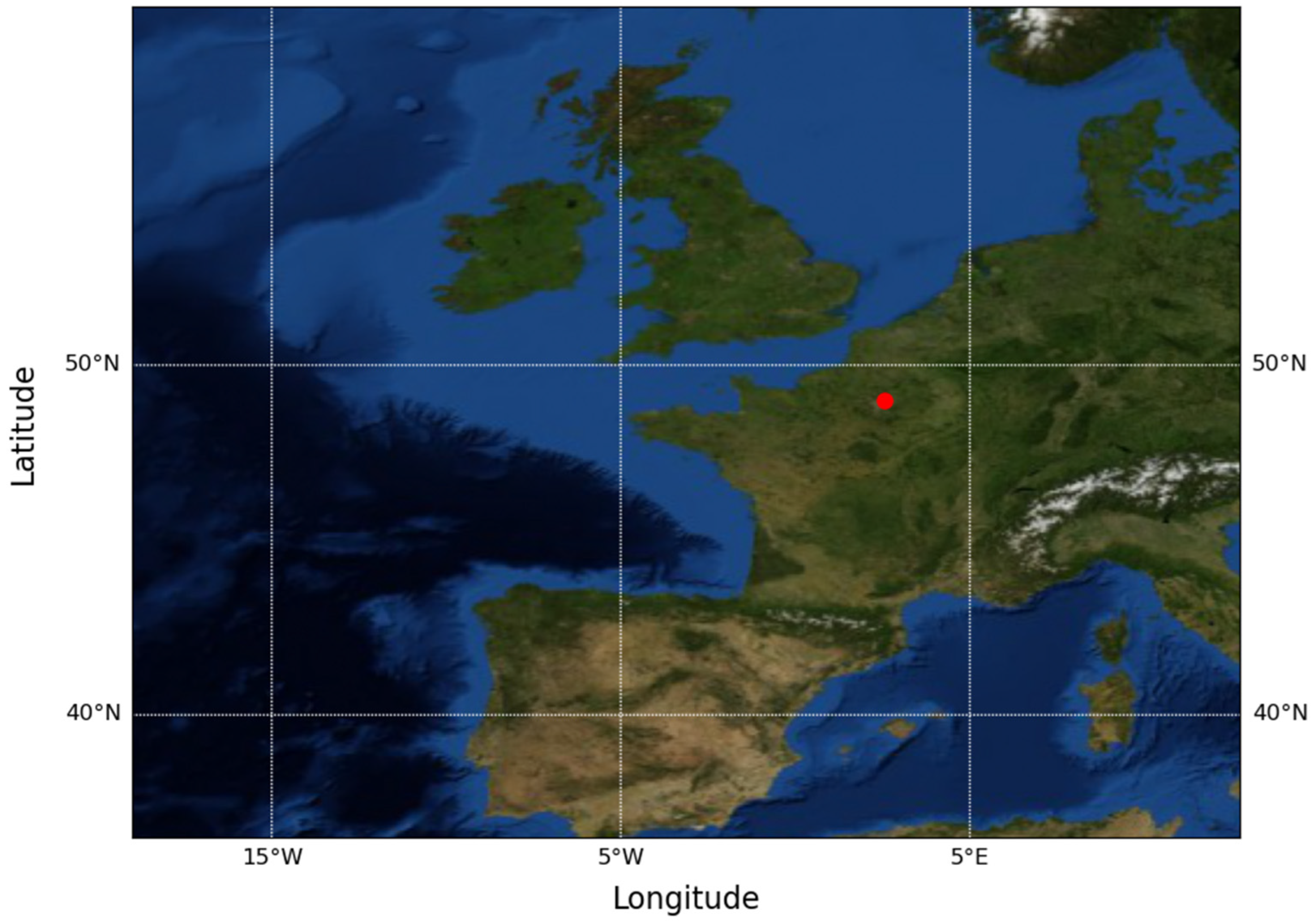
On the other hand, the input features used in training and validation are two-dimensional daily maps of eighteen selected meteorological and hydrological variables (

Table 2. Input features, all from ERA5 reanalysis data; here branch 1 is the branch with smaller kernel and branch 2 with larger kernel in HazeNetb2 shown in Figure 3. Paris local time is UTC + 1.

Short Name	Long Name	Branch in HazeNetb2
REL	Surface relative humidity	1
DREL	Diurnal change in REL, [14:19]mean–[6:12]mean	1
DT2M	Diurnal change of 2 m in temperature	1
T2MS	Daily standard deviation of 2 m in temperature	1
U10	10 m wind, zonal component	1
V10	10 m wind, meridional component	1
TCW	Total column water	1
TCV	Total column water vapor	1
DTCV	Diurnal change in TCV	1
BLH	Height of planetary boundary layer	1
DBLH	Diurnal change in BLH	1
SW1	Volumetric soli water, layer 1	1
SW2	Volumetric soil water, layer 2	1
LCC	Low cloud cover	1
Z500	Geopotential at 500 hPa level	2
D500	Diurnal change in Z500	2
Z850	Geopotential at 850 hPa level	2
D850	Diurnal change in Z850	2

) over a domain of 96 by 128 grids, covering a large part of western Europe, including France, alongside the Atlantic Ocean (Figure 2), obtained from the ERA5 reanalysis data produced by the European Centre for Medium-range Weather Forecasts, or ECMWF [18]. The choice of adopting such a rather large domain serves a dual purpose to identify the regional weather patterns associated with haze and to reduce the influence of noisy small-scale patterns on learning. These chosen variables reflect the general atmospheric and hydrological status under the influence of different weather systems. The horizontal spatial resolution of these maps is 0.25 degrees. The input data have the same number of samples as the labels (i.e., 16,436), though each sample is a 96 by 128 by 18 matrix or image.

2.2. Training–Validation–Evaluation Strategy

Data preparation. The training and validation of the network use the labels and input data covering the period from 1 January 1975 to 31 December 2019. The entire 16,436 pairs of label–input samples were randomly shuffled and then grouped into two sets, with 75% (i.e., 12,327 samples) going to the training set and 25% (4109 samples) going to the validation set. As a common procedure in machine learning and deep learning, input features were normalized into the range of [−1, +1] before training and validation. This normalization of the training set and validation set was performed separately to avoid the leaking of information from the latter to the former. As in [3], these two datasets are hereafter reserved only for their designated purpose in practice. Therefore, the validation result is, in fact, independent of the training process, only serving as a performance indicator.

Training and validation. The training in this study has been conducted in both classification and regression mode. The classification is a two-class training task: class 1 is the LVDs, defined as a day with vis. equal to or lower than the 25th percentile (7.89 km; Table 1) of the long-term (1975 to 2019) observations at CDG, while class 0 is for the other cases. In the regression training mode, the CNN directly predicts a digital value of vis. in km. The two different training modes differ in the activation of the last dense layer (all-connected neural network layer), i.e., sigmoid (2-class) [19] or softmax (multi-class) [20] for the classification, linear for the regression (the activation function is an operator applied to the neurons before being mapped into the next layer of the network to introduce nonlinearity). Their loss functions are also different: a binary cross entropy (categorical cross entropy in multi-class cases) [21] for the classification, while a mean absolute percentage error for the regression. In classification training, since the two classes are imbalanced in terms of the frequency of occurrence, a class weight has been applied to increase the weight of coefficients associated with the much less frequent class 1 (see also [3]).

The training is driven by input features from the training dataset, and the machine is then optimized based on the discrepancy between the training label (i.e., observations in the training dataset) and prediction. This process is continued until the stop point. The length of training, in this study, is at least 2000 epochs (each epoch is a training step that uses the entire training dataset) and is largely independent of the validation performance. This is to force the performance of the network to converge. At the end of each epoch during training, the validation is performed by feeding the entire validation dataset into the machine in training to directly produce predictions, and the scores are derived. The time series of various validation scores can be used to observe the convergence of the machine’s performance during training, as well as for other purposes, such as checking for possible overfitting. The primary scores for classification include precision, recall, and an F1 score; all are statistical metrics particularly useful for imbalanced cases derived based on the so-called confusion matrix (Ref. [3]) since accuracy would be a biased metric for such cases. For regression, the performance is measured by the mean absolute percentage error.

The predictions obtained from the regression training can be presented using the performance metrics of classification as well, i.e., derived based on the predicted hits on different classes using the same class definition in classification mode. This provides a convenient way to compare the performances between the two different training modes using the same metrics, which will be hereafter referred to as regression classification.

Evaluation. In addition to the training–validation procedure, labels, and input features covering the years from 2021 to 2023, totaling 1095 samples obtained from the same data sources and derived in the same procedure as described previously for training and validation data, are also prepared for a separate evaluation of the machines after training. This evaluation is entirely independent of the training–validation procedure since the machines have never had access to this dataset before (training and validation use data from 1975 to 2019). Therefore, it is, in fact, a blind forecasting test using real-world cases. To distinguish this evaluation from the validation, the names used here will be kept in the later discussions.

2.3. Architecture Improvement

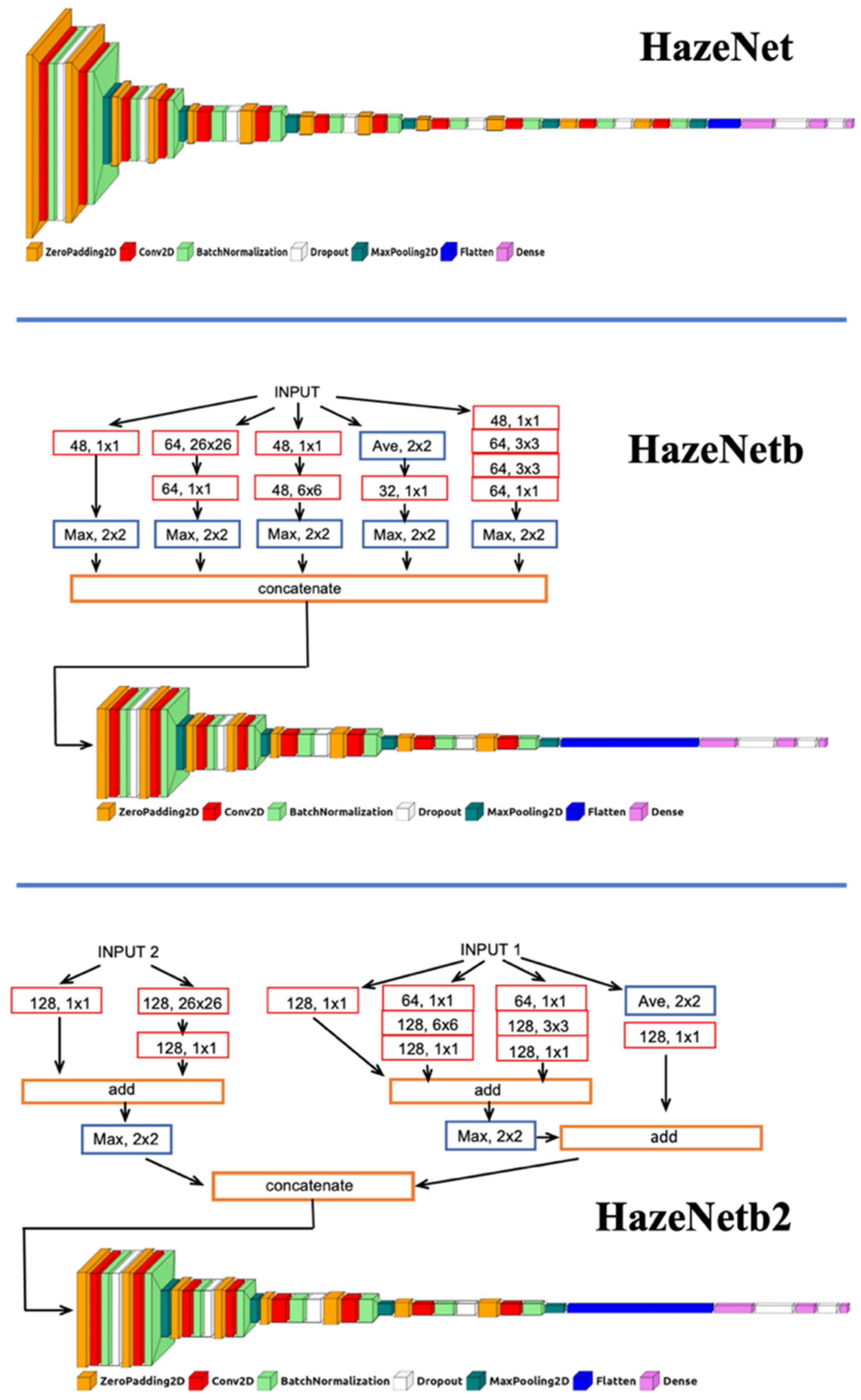
The previous version of HazeNet reported in [3] is a VGG-type [22], 57-layer deep CNN with more than 20 million parameters (Figure 3, the upper panel). Note that the longitudinal–latitudinal data of many meteorological and hydrological variables used in training–validation as input features are actually images with many more channels than the 3-channel RGB images used in common CNN image recognition practices.

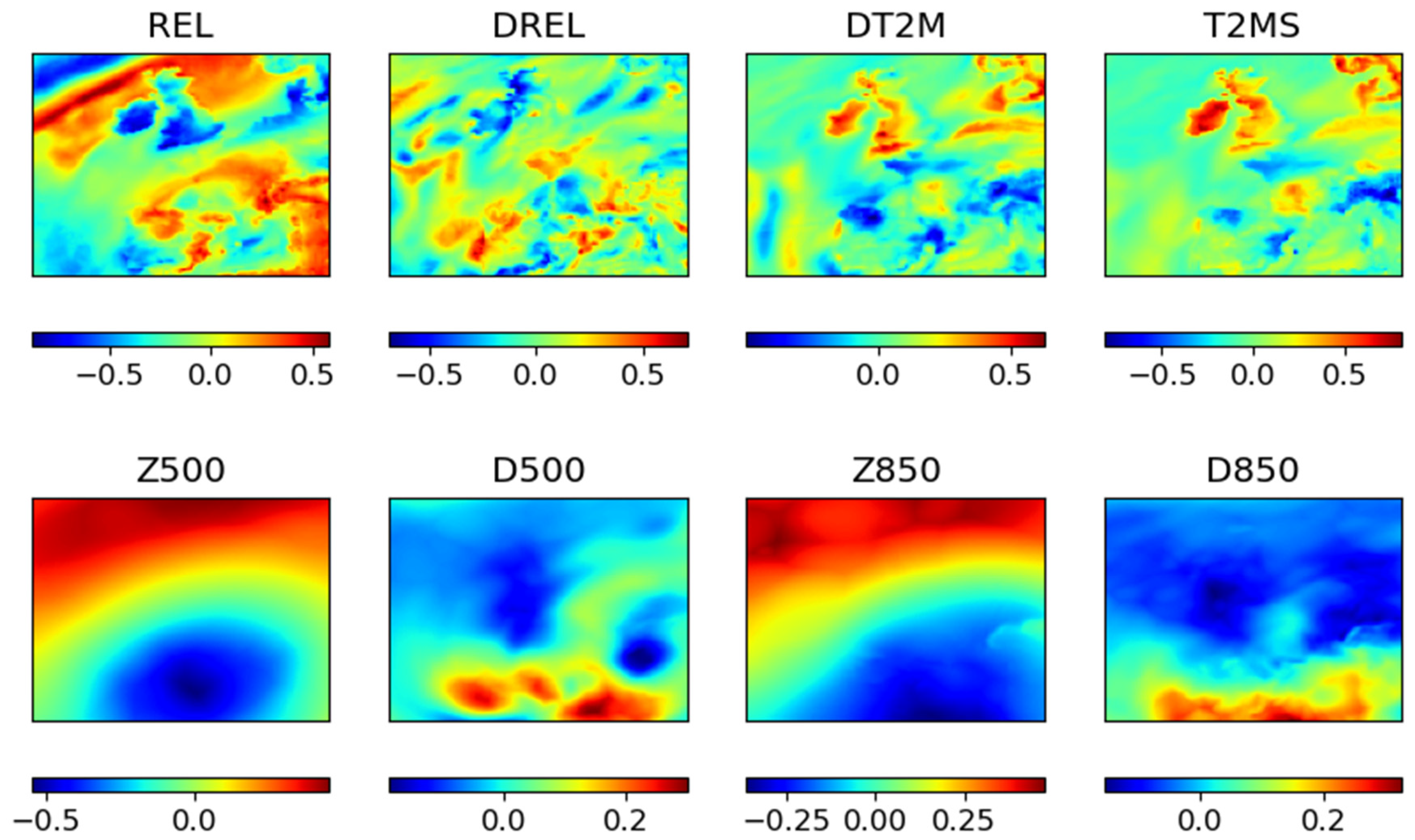
It is well known that the characteristic spatial and temporal scales of meteorological features likely differ from each other [23,24]). For example, the upper panels of Figure 4 are normalized maps of four meteorological variables, from left to right: surface relative humidity (REL) alongside its diurnal change (DREL), a diurnal change of 2m temperature (DT2M), and the daily standard deviation of 2m temperature (T2MS). Each of these figures contains many small spatial-scale patterns, reflecting local weather changes. In contrast, four normalized maps in the lower panels, showing a geopotential at 500 (Z500) and 850 hPa (Z850), along with their corresponding diurnal changes (D500 and D850), respectively, consist of smoothly distributed color belts across many grids. These distributions reflect the characteristics of large-scale atmospheric circulation or weather systems, which evolve much slower than the smaller scale patterns and are less sensitive to the impact factors of the latter, such as clouds, rainfall, boundary layer processes, and so forth, as seen in the upper panels. Therefore, a key issue in making CNN effectively learn these maps involves recognizing patterns of weather or hydrological features with different characteristic spatial scales, which, in many cases, far exceed the pixel level of the maps. Therefore, high resolution at the pixel level, in such cases, is not necessarily the most critical factor in improving the learning, making it a different task from common image recognition projects.

In the previous version of HazeNet (Figure 3, the upper panel), to reduce the difficulty in learning complex weather maps, relatively large kernel sizes were adopted for the first two convolutional layers, despite the additional computational cost. Since the kernel size of a CNN layer decides the grid range of convolution calculation, putting larger kernels in the first two layers can effectively prioritize the learning of less complicated patterns with large and medium spatial scales [3]. The drawback of such a configuration, however, is that it might filter out some smaller-scale features that could be useful in recognizing and distinguishing weather regimes. To better preserve the spatial information on both a large scale and smaller scale contained in different features and thus make the network learn better a wider variety of weather conditions associated with LVEs, two new architectures were introduced in the HazeNet in this study. These new architectures each consisted of two parts; the first part contained certain branches of CNN to process inputs with different kernel sizes, either letting all features be processed together by each branch (Figure 3, the mid-panel, i.e., HazeNetb) or letting features be processed by different branches based on their characteristic scales (Figure 3, the lower panel, i.e., HazeNetb2). Outputs from various branches were then concatenated along the filter dimension and sent to the second part of the network, a VGG-type CNN containing 8 convolution layers with a 3 × 3 kernel, taken from the bottom part of the original HazeNet (see [3] for details). The new architectures are apparently inspired by the ideas of Inception Net [25], ResNet [26], and a 1 × 1 layer, or ‘network in network’ [27], for various designated purposes. Multiple parallel branches with different kernel sizes can lead to the effective learning of pixel-wise patterns or channel-wise correlations, sharing certain ideas with the attention module for image recognition [28].

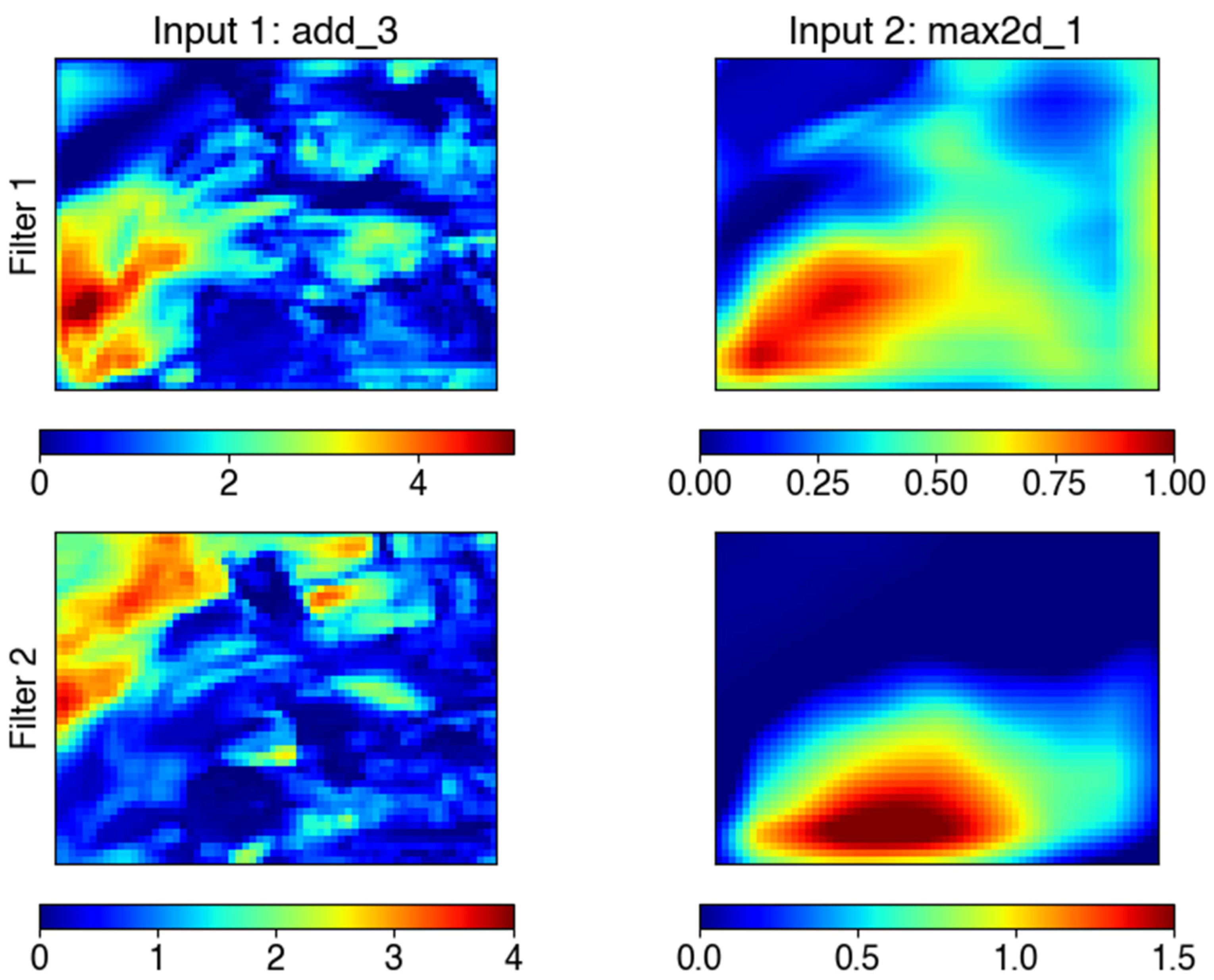
Figure 5 shows the outputs of the second convolutional layer (just before the 3 × 3 kernel layer) in the original HazeNet. The displayed patterns contain the color blocks that are likely defined by the features with larger spatial scales while still carrying certain signatures of the smaller-scale features. On the other hand, from the result of the branched HazeNetb (Figure 6), the output of each branch clearly displays a pattern with the prioritized characteristic scale enforced by its kernel size. Additionally, it can be seen from the outputs of HazeNetb2 in Figure 7 that such an effect can be further enhanced by arranging different features to go through different branches based on their characteristic scales.

Besides the benefit of better-preserving patterns with different characteristic scales, the branched architectures can also lower the complexity of the machine. For instance, the total parameters of about 20 million in HazeNet have been reduced to nearly 11 million in HazeNetb, and further to 10.6 million in HazeNetb2. However, due to the utilization of large kernel sizes, the training time of branched machines is longer than that of HazeNet, with a nearly 10% increase in HazeNetb and a 40% increase in HazeNetb2 compared to that of HazeNet. Each training of the branched architectures requires 33 to 45 GPU hours using an Nvidia Tesla V100 GPU, depending on the configuration.

3. Performance in Validation of Trained Machines

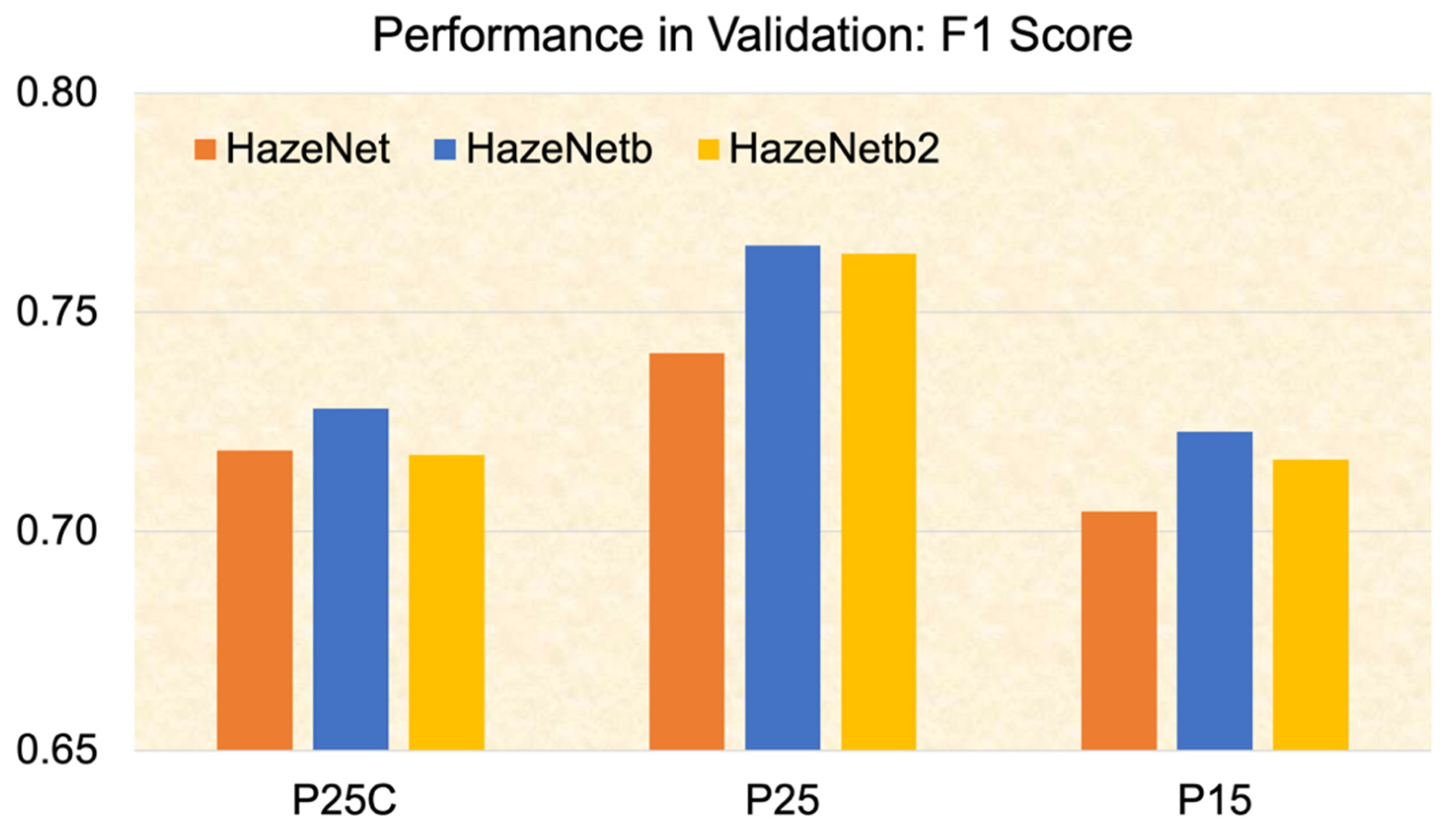
The previously described training strategy has led to the production of stable validation scores at the end of each training session and made the performance comparison between machines with different configurations more objective (Figure 8). Note that each validation, whenever conducted, uses the entire validation dataset and consists of nearly 12 years’ worth of observations. The performances of various versions of HazeNet in validation clearly indicate that the two branched architectures have both delivered better F1 scores in the regression–classification mode for events with vis. equal or lower than the 25th, 20th, and 15th percentiles than the non-branched version, while the latter performed better for events equal or lower than the 10th and 5th percentiles of the long-term observations (Figure 9 and

Table 3. The validation performances of HazeNet with different architectures in classification and regression–classification. Shown are last 100-epoch means. The best scores are highlighted with bold font.

	Accuracy	Precision	Recall	F1-Score
Classification (P25C)
HazeNet	0.851	0.717	0.721	0.719
HazeNetb	0.858	0.732	0.724	0.728
HazeNetb2	0.854	0.726	0.718	0.722
Regression–Classification (P25)
HazeNet	0.875	0.815	0.680	0.741
HazeNetb	0.885	0.826	0.713	0.765
HazeNetb2	0.882	0.806	0.725	0.763
Regression–Classification (P20)
HazeNet	0.892	0.800	0.679	0.734
HazeNetb	0.896	0.811	0.683	0.742
HazeNetb2	0.894	0.796	0.694	0.742
Regression–Classification (P15)
HazeNet	0.905	0.750	0.665	0.705
HazeNetb	0.913	0.784	0.670	0.723
HazeNetb2	0.909	0.756	0.681	0.716
Regression–Classification (P10)
HazeNet	0.928	0.722	0.586	0.647
HazeNetb	0.925	0.735	0.530	0.616
HazeNetb2	0.926	0.733	0.547	0.627
Regression–Classification (P5)
HazeNet	0.952	0.698	0.342	0.459
HazeNetb	0.950	0.721	0.255	0.377
HazeNetb2	0.952	0.759	0.272	0.400

). The evolution of regression–classification scores with the probability of targeted LVEs shown in Table 3 demonstrates that the accuracy of all machines increases with the lowering of probability, indicating the effect of increasing the imbalance (i.e., the ratio of non-targeted to targeted events). On the other hand, the F1 score decreases with probability, implying the forecasting skill of the machines is lower in low-probability cases than in higher ones. In comparison, in the regular classification, the difference between these three architectures is rather smaller. Note here that to smooth out potential small variations in performance metrics along the training progression, the quantities of metrics shown in Figure 9 and Table 3 are their last 100-epoch means.

On the other hand, the predicted vis. by all trained regression machines have demonstrated statistically significant (with nearly zero p values) correlations with the observations contained in more than 12 years’ worth of validation data, with an R² of 0.54, 0.61, and 0.59 for HazeNet, HazeNetb, and HazeNetb2, respectively. The performances of the two branched versions are, again, better than that of the original HazeNet. The performance in regression could be a likely reason behind the outcome, as all machines in the regression classification mode, regardless of adopted architecture, have produced better performances in validation than their twins trained in pure classification mode (Figure 9 and Table 3). The advantage of regression–classification machines is primarily reflected in their precision scores, i.e., the ratio of true-to-total predicted LVDs, while their recall scores (ratio of predicted to total observed LVDs) stayed nearly the same as in the classification mode (Table 3). In other words, the regression–classification forecasts are made by using predicted vis. quantities from regression have mainly led to a reduction in the so-called false positive (false alarm) cases in comparison to the results of the trained classification machines, implying that the latter might tend to be confused by the similar weather patterns associated with cases across the definition line of LVDs.

The best forecast performer among the three versions of HazeNet in validation was HazeNetb. The other branched architecture, HazeNetb2, generally performed better than the original HazeNet, particularly in the regression–classification mode, and produced close but slightly lower scores than HazeNetb, possibly due to its more complicated structure, which might require longer training and certain additional optimizations. Considering the required training time, HazeNetb apparently possesses the edge among the three architectures in terms of cost–benefit. Note that the similar advantage of branched architecture over the non-branched one is also found in the testing of previously studied cases in Beijing and Shanghai.

4. Evaluation of the Trained Machines Using 2021 and 2023 Data

Up to this point, all the training and validation have been performed using historical data from 1975 to 2019, while the performance of the trained machines using data beyond the training and validation dataset is still unknown. To further evaluate the performance of HazeNet, a “blind forecast” evaluation of various trained HazeNet versions has been conducted by feeding them with data from the year 2021 to 2023 to produce predictions. Note that the data used in the evaluation have not been utilized in the training–validation procedure. During these three years (i.e., 1095 days), there were, in total, 118 LVDs observed at the CDG site with a vis. lower or equal to P25 or 7.89 km. Machines trained in both the classification and regression–classification modes have been evaluated. Note that this is just a limited evaluation of the performance of trained machines with real-world data beyond their training dataset. Only the long-term use of the machines driven by real-time forecasting data, perhaps, could better evaluate the machines while improving them continuously through re-training.

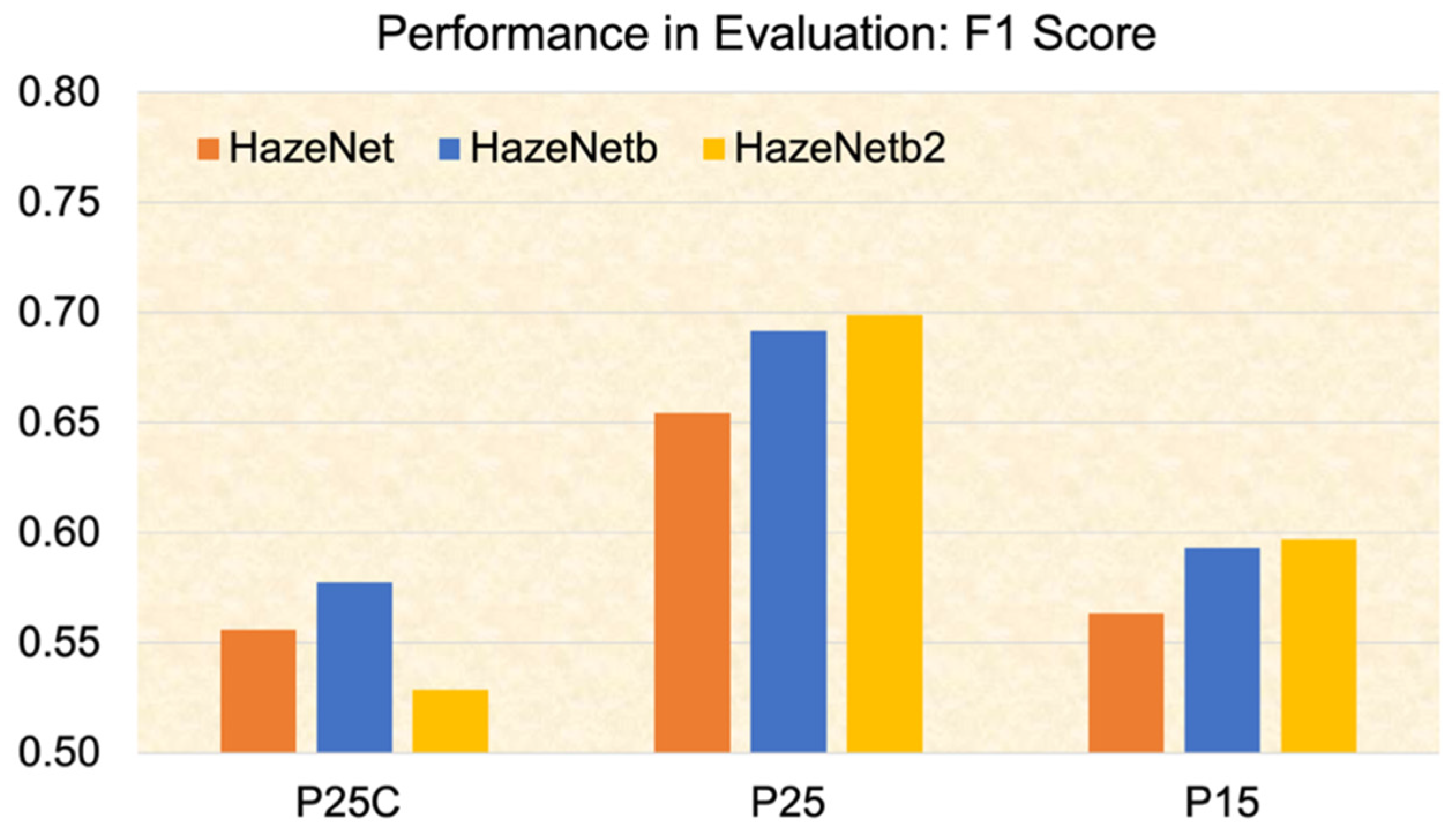
The evaluation results suggest that both branched architectures have achieved better performance in both the classification mode and regression–classification mode compared to the original HazeNet (Figure 10 and

Table 4. The performances of different network architectures in evaluation (data of year 2021–2023). The best scores are highlighted with bold font.

	HazeNet	HazeNetb	HazeNetb2
Mean absolute percentage error (%)	10.02	9.82	9.92
R2	0.53	0.58	0.54
F1 score of P25C	0.56	0.58	0.53
F1 score of P25	0.65	0.69	0.70
F1 score of P20	0.67	0.65	0.66
F1 score of P15	0.56	0.59	0.60
F1 score of P10	0.54	0.47	0.51

Note: Correlations between predicted and observed surface visibility by three machines are all statistically significant since p values are all practically zero. P25 P20, P15, and P10 represents the LVDs defined with daily vis. lower or equal to the 25th, 20th, 15th, and 10th percentile of long-term observations (118, 78, 55, and 26 LVDs), respectively, derived from regression–classification. While P25C is the same as P25 except for direct classification. All the machines did not show any skill in predicting P5 events, which only has 3 such observed LVDs.

). The F1 score of the branched architecture is about 4–5% higher than that of the original HazeNet in the classification mode (P25C) and 6–7% higher in the regression–classification mode (P25). The performance improvements achieved by branched architectures in evaluation, particularly in the regression–classification mode, are even more significant than those reflected in the validation. Comparing the two branched architectures, HazNetb2 delivered a slightly higher F1 score than HazeNetb in the regression–classification mode, while the latter performed better in classification. Again, the regression–classification machines, regardless of the adopted architecture, achieved F1 scores of about 10% or higher compared to those obtained by their classification twins. Like the finding in the validation analysis, the advantage of the regression–classification machines in the precision score is much more evident than in the recall score. For example, in the case of HazeNetb2, precision is 0.66 versus 0.42, and recall is 0.74 versus 0.70 in regression–classification versus classification, respectively. Regarding the scores of regressions machines before being translated into classification metrics, HazeNetb2 produced a 9.92% mean absolute percentage error, while HazeNetb obtained 9.82%; both were lower than the same metrics of HazeNet in 10.02%. The evaluation results also demonstrate, as shown in Table 4, that the performances of all machines generally degrade as the probability of targeted events decreases.

The observed versus predicted vis. in quantities by the trained branched machine of HazeNetb2 are displayed in Figure 11. Firstly, the machine has produced a seasonality of LVEs in Paris that matches the observed result very well. Secondly, the point-to-point comparison between the predicted and observed vis. show a rather small overall discrepancy, indicating that the machine has captured an observed evolution of vis. reasonably well. For LVDs defined with a vis. equal or lower than P25 (marked in Figure 11b with a solid black line), HazeNetb2 has captured 70% of the observed events during the three-year period (or a recall of 0.70 in terms of regression–classification mode metric), while 74% of the predicted LVDs are true cases based on observations (precision = 0.74). Its accuracy in forecasting both LVDs and no-haze cases is 93%, evidently exceeding the frequency of non-haze events of 89%, i.e., the no-skill score in a highly imbalanced classification forecast obtained by predicting solely in the overwhelming class. Note that though a model like HazeNet would be unlikely to achieve a perfect score in forecasting the occurrence of haze, because such occurrence is not determined by the weather conditions alone. Mitigation measures enforced by policy decisions, for example, could reduce, if not eliminate, the chance for haze to appear in many cases.

5. Summary and Conclusions

A deep-learning platform, HazeNet, has been developed to forecast the occurrence of low-visibility events or hazes in the Paris area. To better preserve the information regarding the characteristic spatial scales of different features in training, two branched architectures have recently been developed. These machines have been trained and validated using multi-decadal (1975–2019) daily regional maps of eighteen meteorological and hydrological variables as input features and surface visibility observations as the targets. The goal was to train the deep CNNs to recognize various regional weather and hydrological regimes associated with the occurrence of low-visibility events in the greater Paris area.

The branched architectures have reduced the number of total parameters of the machines from more than 20 million in the original non-branched version of HazeNet to just above 10 million. While the computational expense in training these branched machines is clearly increased, the introduction of the branched architectures has improved the performance of the CNNs in validation and, more evidently, in an evaluation using the most recent observational data from 2021 to 2023, which have never been used in training and validation. As an example, one of the trained machines with branched architecture (i.e., HazeNetb2) has successfully predicted 70% of the observed low-visibility events during the three-year period at Paris Charles de Gaulle Airport. Among those predicted low-visibility events by the machine, 74% of them are true cases based on observation. Another interesting result is that the regression–classification machines (using predicted visibility in quantity from regression to make class-based forecast), regardless of adopted architecture, are apparently favored, rather than their trained classification twins based on the performances in validation and evaluation. A major reason behind this is that the pure classification machines tend to produce a higher number of false alarms, i.e., a lower precision than regression–classification machines do, likely due to confusion on the similar weather patterns possessed by certain events on different sides of the LVD definition line. This result thus suggests training a regression machine first, even for performing a class-based forecast of hazes. Combining the required training time and performance, the branched HazeNetb appears to be the architecture to pick among the three from a cost–benefit point of view.

It is worth indicating that the performance in the validation and evaluation of HazeNet reflects statistics of performance metrics obtained from a forecast of about 15 years of real-world cases. Its skill comes from learning using more than 30 years of observational data that are independent of the ones used in validation and evaluation. Jointly, these cases cover nearly all the observations that are useful and available to this study. An additional benefit of machines like HazeNet is that they can be progressively re-trained and thus further improved whenever the most recent observations or any new type of useful data become available. An interesting fact to note, though, is that the machines like HazeNet (which could extend to traditional deterministic atmospheric models too) developed to only use weather conditions as the input for haze forecasting would be unlikely to achieve a perfect score, owing to, e.g., the implementation of certain air-pollution mitigation measures. In addition, a trained HazeNet is only for applications in the targeted area. It needs to be re-trained for anywhere else.

An interesting question regarding the deep-learning machine is whether any specific input feature (s) appears to be more important than others to the performance. This has been partially explored for the branched HazeNet, where 11 features were firstly selected from the original 18 based on a comparison of pattern-similarity between each pair of features throughout the entire dataset; then, the machines were trained and validated using the input with reduced features. The result showed that the machines trained with a reduced input set did not suffer an evident performance setback compared to the scores achieved by their 18-input counterparts. However, more experiments are still needed to evaluate the generalization of such a feature selection method [29]. Apparently, the performance of the branched CNNs can be further improved through, e.g., architecture optimization or parameter tuning. Such an extensive effort, however, clearly exceeds the scope of the current exploratory study and could be accomplished in a future effort.

References

1. Willet, H.C. Fog and haze, their causes, distribution, and forecasting. Mon. Weather Rev. 1928, 56, 435–468. [Google Scholar] [CrossRef]
2. Lee, H.-H.; Bar-Or, R.; Wang, C. Biomass burning aerosols and the low visibility events in Southeast Asia. Atmos. Chem. Phys. 2017, 17, 965–980. [Google Scholar] [CrossRef]
3. Wang, C. Forecasting and identifying the meteorological and hydrological conditions favoring the occurrence of severe hazes in Beijing and Shanghai using deep learning. Atmos. Chem. Phys. 2021, 21, 13149–13166. [Google Scholar] [CrossRef]
4. Day, D.E.; Malm, W.C. Aerosol light scattering measurements as a function of relative humidity: A comparison between measurements made at three different sites. Atmos. Environ. 2001, 35, 5169–5176. [Google Scholar] [CrossRef]
5. Hyslop, N.P. Impaired visibility: The air pollution people see. Atmos. Environ. 2009, 43, 182–195. [Google Scholar] [CrossRef]
6. Bergot, T.; Terradella, E.; Cuxart, J.; Mira, A.; Liechti, O.; Mueller, M.; Nielsen, N.W. Intercomparison of single column numerical models for the prediction of radiation fog. J. Appl. Meteorol. Clim. 2007, 46, 504–521. [Google Scholar] [CrossRef]
7. Marzban, C.; Leyton, S.; Colman, B. Ceiling and visibility forecast via neural networks. Weather Forecast. 2007, 22, 466–479. [Google Scholar] [CrossRef]
8. Dutta, D.; Chaudhuri, S. Nowcasting visibility during wintertime fog over the airport of a metropolis of India: Decision tree algorithm and artificial neural network approach. Nat. Hazards 2016, 75, 1349–1368. [Google Scholar] [CrossRef]
9. Castillo-Botón, C.; Casillas-Pérez, D.; Casanova-Mateo, C.; Ghimire, S.; Cerro-Prada, E.; Gutierrez, P.A.; Deo, R.C.; Salcedo-Sanz, S. Machine learning regression and classification methods for fog events prediction. Atmos. Res. 2022, 272, 106157. [Google Scholar] [CrossRef]
10. Zhang, Y.; Wang, Y.; Zhu, Y.; Yang, L.; Ge, L.; Luo, C. Visibility prediction based on machine learning algorithms. Atmosphere 2022, 13, 1125. [Google Scholar] [CrossRef]
11. Gagne, D.J., III; Haupt, S.E.; Nychka, D.W.; Thompson, G. Interpretable deep learning for spatial analysis of severe hailstorms. Mon. Weather Rev. 2019, 137, 2827–2856. [Google Scholar] [CrossRef]
12. Chattopadhyay, A.; Nabizadeh, E.; Hassanzadeh, P. Analog forecasting of extreme-causing weather patterns using deep learning. J. Adv. Model. Earth Syst. 2020, 12, e2019MS001958. [Google Scholar] [CrossRef]
13. Chen, K.; Zhou, Y.; Ren, T.; Li, X. Short-term sea fog area forecast: A new data set and deep learning approach. J. Geophys. Res. Mach. Learn. Comput. 2024, 1, e2024JH000230. [Google Scholar] [CrossRef]
14. Yang, N.; Wang, C.; Li, X. Improving tropical cyclone precipitation forecasting with deep learning and satellite image sequencing. J. Geophys. Res. Mach. Learn. Comput. 2024, 1, e2024JH000175. [Google Scholar] [CrossRef]
15. Wang, C. Exploiting deep learning in forecasting the occurrence of severe haze in Southeast Asia. arXiv 2020. [Google Scholar] [CrossRef]
16. Smith, A.; Lott, N.; Vose, R. The integrated surface database: Recent developments and partnerships. Bull. Am. Meteorol. Soc. 2011, 92, 704–708. [Google Scholar] [CrossRef]
17. Wang, C. A modeling study on the climate impacts of black carbon aerosols. J. Geophys. Res. 2004, 109, D03106. [Google Scholar] [CrossRef]
18. Hersbach, H.; Bell, B.; Berrisford, P.; Hirahara, S.; Horányi, A.; Muñoz-Sabater, J.; Nicolas, J.; Peubey, C.; Radu, R.; Schepers, D.; et al. The ERA5 global reanalysis. Q. J. R. Meteorol. Soc. 2020, 146, 1999–2049. [Google Scholar] [CrossRef]
19. Han, J.; Morag, C. The influence of the sigmoid function parameters on the speed of backpropagation learning. In From Natural to Artificial Neural Computation; Lecture Notes in Computer Science; Mira, J., Sandoval, F., Eds.; Springer: Berlin/Heidelberg, Germany, 1995; Volume 930, pp. 195–201. [Google Scholar] [CrossRef]
20. Bridle, J.S. Probabilistic interpretation of feedforward classification network outputs, with relationships to statistical pattern recognition. In Neurocomputing: Algorithms, Architectures and Applications; NATO ASI Series (Series F: Computer and Systems Sciences); Soulié, F.F., Hérault, J., Eds.; Springer: Berlin/Heidelberg, Germany, 1990; Volume 68, pp. 227–236. [Google Scholar] [CrossRef]
21. Hinton, G.E.; Salakhutdinov, R.R. Reducing the Dimensionality of Data with Neural Networks. Science 2006, 313, 504–507. [Google Scholar] [CrossRef]
22. Simonyan, K.; Zisserman, A. Very deep convolutional networks for large-scale image recognition. arXiv 2015. [Google Scholar] [CrossRef]
23. Holton, J.R. An Introduction to Dynamic Meteorology, 4th ed.; Elsevier Academic Press: Boston, MA, USA, 2004; 535p. [Google Scholar]
24. Markowski, P.; Richardson, Y. Mesoscale Meteorology in Midlatitudes; Willey-Blackwell: West Sussex, UK, 2010; 430p. [Google Scholar]
25. Szegedy, C.; Vanhoucke, V.; Ioffe, S.; Shlens, J.; Wojna, Z. Rethinking the inception architecture for computer vision. arXiv 2015. [Google Scholar] [CrossRef]
26. He, K.; Zhang, X.; Ren, S.; Sun, J. Deep residual learning for image recognition. arXiv 2015. [Google Scholar] [CrossRef]
27. Lin, M.; Chen, Q.; Yan, S. Network in network. arXiv 2014. [Google Scholar] [CrossRef]
28. Wang, H.; Wang, S.; Qin, Z.; Zhang, Y.; Li, R.; Xia, Y. Triple attention learning for classification of 14 thoracic diseases using chest radiography. Med. Image Anal. 2021, 67, 101846. [Google Scholar] [CrossRef]
29. Wang, C. A branched deep convolutional neural network for forecasting the occurrence of hazes in Paris using meteorological maps with different characteristic spatial scales. arXiv 2023. [Google Scholar] [CrossRef]
Figure 1. Daily average surface visibility in km observed at Paris Charles de Gaulle Airport (CDG) since 1975. An unknown systematic switch in statistics occurred during 2000–2002 (the 25th to 27th year after 1975) that affects mostly on the results in the clear (high percentile) than haze (low percentile) days.
Atmosphere 15 01239 g001
Figure 2. The data domain of meteorological and hydrological input features, consisting of 96 latitudinal and 128 longitudinal grids with an increment of 0.25 degree. The red dot marks the location of Charles de Galle Airport.
Atmosphere 15 01239 g002
Figure 3. Diagrams of various architectures of HazeNet. Here Max represents a MaxPooling layer, Ave is an Average layer. For 2D convolutional layer, “128, 1 × 1” represents a layer with 128 filter sets and a kernel size of 1 × 1. Each convolutional layer is followed by a batch normalization layer unless otherwise indicated. The bottom part in HazeNetb and HazeNetb2 is a CNN consisting of 8-convolutional layers with 3 × 3 kernels, adopted from the last part of original HazeNet (see [3]). Part of the charts were drawn using visualkeras package (Gavrikov, P., 2020, https://github.com/paulgavrikov/visualkeras; accessed on 14 October 2024).
Atmosphere 15 01239 g003
Figure 4. Examples of normalized maps (96 by 128 pixels) of meteorological features with different characteristic spatial scales. See Table 2 for the description of plotted features.
Atmosphere 15 01239 g004
Figure 5. The outputs (62 by 94 pixels) of the first four filters from the second convolutional layer (6 × 6 kernel) in HazeNet. Different color scales are used for various panels to highlight their distributions.
Atmosphere 15 01239 g005
Figure 6. The outputs of various branches of HazeNetb just before the concatenate layer (Ref. Figure 3), shown are those of the first filter set, each has 48 by 64 pixels. Different color scales are used for various panels to highlight their distributions.
Atmosphere 15 01239 g006
Figure 7. (Left) The outputs from the small kernel branch (input1) just before the concatenate layer of HazeNetb2, shown only the first two filter sets. (Right) The same but for the outputs from the large kernel (input2) branch. Each panel has 48 by 64 pixels. Different color scales are used for various panels to highlight their distributions.
Atmosphere 15 01239 g007
Figure 8. Dynamically calculated validation scores of statistical performance metrics with training progression in a classification training of HazeNetb. Each score point represents statistics of results calculated using the entire validation dataset. Here Acc and Loss represent the accuracy and loss in training, respectively, VAcc and VLoss the same metrics but in validation; while others are all validation scores commonly used in classification forecasting: precision, recall, and F1 score have a range of [0, 1], ETS is the equitable threat score with a range of [−1/3, 1], and HSS is the Heidke skill score ([−inf, 1]), all derived based on the so-called confusion matrix (Ref. [3]) for their definitions).
Atmosphere 15 01239 g008
Figure 9. The F1 scores of machines with different architectures obtained from the end of training session validation (last 100-epoch means). Here P25C represents the results from classification mode for events with vis. equal or lower than the 25th percentile of long-term observations, while P25 and P15 are the results from regression–classification mode, here P15 is for events with vis. equal or lower than the 15th percentile of long-term observations.
Atmosphere 15 01239 g009
Figure 10. The same as Figure 9 but for performance of various machines in the evaluation using data from 2021 to 2023.
Atmosphere 15 01239 g010
Figure 11. Evaluation results of HazeNetb2 using data from 2021 to 2023: (a) a scatter plot of predicted versus observed quantities of vis. in km; and (b) the same comparison but displayed as time series. Total number of LVD (P25) during the 3-year period is 118.
Atmosphere 15 01239 g011