The Influence of PE Initial Field Construction Method on Radio Wave Propagation Loss and Tropospheric Duct Inversion

Abstract

Parabolic equations (PE) are commonly employed for calculating the spatial propagation loss of wireless signals. The initial field is a crucial factor. To investigate the impact of construction accuracy on the calculation of radio wave propagation loss, we selected the half-wave dipole antenna and its Gaussian approximation to examine the influence of wide-angle PE modeling. We analyzed the disparities between the actual antenna pattern and the Gaussian beam approximation, as well as the discrepancies in the corresponding initial field and the calculation of radio wave propagation loss in PE modeling. The simulation results indicate that the error of the Gaussian approximation increases as the angle of departure from the antenna main beam increases, with a relative error of approximately 30% in the initial field. A comparison between the experimental test of the broadcast signal and the simulation calculation reveals that the model based on the actual antenna aligns more closely with the measured value on a flat underlying surface. However, in mountainous areas with significant fluctuations, the simulation results are consistent with each other and higher than the measured value. The inversion results obtained through the particle swarm optimization algorithm demonstrate that the model based on the actual antenna exhibits superior inversion accuracy for the tropospheric atmospheric duct structure.

1. Introduction

The design and operation of wireless transmission systems require a reasonable and effective evaluation and prediction of propagation losses within their coverage area. Among these systems, wave propagation modeling based on the parabolic equation is widely used in radar, communication, broadcast systems, and remote sensing inversion research [1,2]. In the process of PE modeling, the construction of the initial antenna field is a crucial factor that affects simulation accuracy. The initial field corresponds to the transmitting antenna radiation field in the actual communication system, and the antenna beam approximation method is used to construct the initial field in the research and application of radio wave propagation. The accuracy of PE modeling decreases with an increase in the beam angle due to the difference in the beamwidth of the actual transmitting antenna. To address this issue, PE modeling has been developed from narrow-angle parabolic equations to wide-angle parabolic equations. Hardin and Tappert first used Taylor approximation to construct narrow-angle parabolic equations for differential operators, and as the application scenarios of PE expanded, the wide keratalization of differential operators was also developed [3]. The Claerbout approximation was initially applied in geophysics and later introduced into the field of radio wave propagation due to its universality [4]. The Feit–Fleck approximation originated from the study of Feit and Fleck in optical fiber sensing [5] and was later applied to the study of radio wave propagation by Thomson and Chapman [6], which is suitable for the parabolic equation split-step Fourier transform method. Greene’s approximation, developed later, significantly broadens the beam range of PE, with an angle of up to 40° relative to the horizontal plane, and effectively controls the relative error caused by the approximation of differential operators [7]. The development of these differential operator approximation methods has increased the application scenarios of PE wave propagation modeling. However, it has also reduced the accuracy of the Gaussian beam method, which was originally suitable for narrow-angle initial field approximation.

When using a Gaussian approximate narrow-beam transmitting antenna, the main beamwidth is generally within 15°. For such beamwidths, even considering the influence of sidelobes, the accuracy of adopting a Gaussian approximate transmitting antenna main beam is very high, and relevant research has been widely applied [8,9,10,11]. However, in actual wireless transmission systems, the main beamwidth of the transmitting antenna is often more than 15°, especially in scenes larger than 40°. Therefore, it is necessary to evaluate the impact of increasing the main beam of the Gaussian approximation to actual transmitting antenna. In addition to studying the error of the PE equation with different beamwidths, the error analysis of Gaussian approximation has also been reported [12,13]. Particularly, in the beam scanning of MIMO and other applications [14], the main beam of the antenna will deviate from the zero-degree direction of the PE model at a larger angle, and the propagation loss of space radio waves within the coverage range will pose new challenges to the angle problem in PE modeling. Therefore, it is necessary to explain the difference between the PE model and the real antenna after using Gaussian approximation. Currently, there have been relevant studies on the construction of the initial field of the transmitting antenna using Gaussian approximation, but they are limited to the error analysis of the applicable angle range of the PE method [15]. This paper presents detailed results of simulation calculations and actual measurements to verify the radio wave propagation loss caused by the Gaussian approximation of the transmitting antenna involving a wider angle.

Based on the above analysis, this paper focuses on four research aspects: (1) the difference between the actual antenna and its Gaussian approximate antenna pattern; (2) the difference between PE initial fields constructed based on antenna patterns; (3) the influence of two PE initial field construction methods on the simulation calculation of radio wave propagation losses within the coverage area; (4) the accuracy of the propagation model constructed by the two methods for retrieving the tropospheric duct structure. The specifics of the different sections of the article are listed below: Section 2 presents the wide-angle PE equation theory, a comparison of Gaussian beam approximation, and the half-wave dipole antenna pattern. In Section 3, the initial fields corresponding to the two types of antenna patterns and the propagation simulation in the PE model are calculated and compared, and the differences in the initial fields and their influence on the radio wave propagation calculation are explained. Section 4 describes the actual test scenarios and test results, comparing the measured results with the calculated results of the propagation loss in the PE model using the two initial fields. Section 5 employs particle swarm optimization (PSO) for a comparative analysis of atmospheric profile inversion. Finally, Section 6 provides the research conclusions.

2. PE Model Theory of Radio Wave Propagation

2.1. Wide Angle PE Wave Propagation Model

In this paper, a two-dimensional parabolic equation model of radio wave propagation for wireless transmission signals is presented. The field component ψ satisfies the two-dimensional scalar wave Equation (1):

$$\frac{{\partial }^2\psi }{\partial x^2}+\frac{{\partial }^2\psi }{\partial z^2}+k^2{n}^2\psi =0$$

(1)

where k is the free space wavenumber; n is the free-space refractive index. For horizontal polarization, the appropriate field component $\Psi$ is defined by $\Psi \left(x,z\right)=E_y\left(x,z\right)$, and for vertical polarization, by $\Psi \left(x,z\right)=H_y\left(x,z\right)$.

The wave function propagating in the forward direction is

$$u(x,z)=e^{-ikx}\psi (x,z)$$

(2)

Substituting Equation (2) into Equation (1) and ignoring the variation in n with x, Equation (1) can be factored as

$$[\frac{\partial }{\partial x}+ik(1-Q)][\frac{\partial }{\partial x}+ik(1+Q)]u=0$$

(3)

In this equation, the former factor represents forward propagation, and the latter represents backward propagation. The pseudo-differential operator Q is defined by

$$Q=\sqrt{\frac{1}{k^2}\frac{{\partial }^2}{\partial z^2}+n^2}$$

(4)

The forward propagation part is retained, and the wide-angle parabolic equation constructed by Greene approximation is as follows [16]:

$$\frac{{\partial }^{3}u}{\partial z^2\partial x}+\frac{ik(d-b)}{d}\frac{{\partial }^{2}u}{\partial z^2}+k^2[\frac{c}{d}+(n^2-1)]\frac{\partial u}{\partial x}+i{k}^3[\frac{c-a}{d}+(1-\frac{b}{d})(n^2-1)]u=0$$

(5)

The finite difference method is used to simplify Equation (5), whose difference mesh is the Crank–Nicolson scheme. $u\left(x_m,z_j\right)$ is simply denoted as $u_j^m$, and Equation (5) is further simplified as

$$A{u}_{j-1}^m+C_{j-1}^m{u}_j^m+A{u}_{j+1}^m=D{u}_{j-1}^{m-1}+F_{j-1}^{m-1}{u}_j^{m-1}+D{u}_{j+1}^{m-1}$$

(6)

$$\left\{\begin{array}{l}A=2d+ik\Delta x(d-b)\\ B=2c+ik\Delta x(c-a)\\ C_j^m=-2A+k^2\Delta z^2[B+A{(n_j^m)}^2-A]\\ D=2d-ik\Delta x(d-b)\\ E=2c-ik\Delta x(c-a)\\ F_j^m=-2D+k^2\Delta z^2[E+D{(n_j^m)}^2-D]\end{array}\right.$$

(7)

$$u_m=({(AC)}^{-1}\cdot DF)u_{m-1}$$

(8)

In the Equations (6)–(8), the constant $a$ = 0.99987; $b$ = 0.79624, and $c$ = 1, $d$ = 0.30102. After calculating the initial field, the propagation loss of the whole field can be solved iteratively. Turkey absorption window function was used for the upper boundary [17]:

$$w(z)=\left\{\begin{array}{l}1,0\le z\le \frac{3}{4}{z}_{\max }\\ \frac{1}{2}+\frac{1}{2}\cos [4\pi (z-\frac{3}{4}{z}_{\max })],\frac{3}{4}{z}_{\max }\le z\le z_{\max }\end{array}\right.$$

(9)

The Leontovich boundary conditions were used for the lower boundary [18]:

$${\left.\frac{\partial u(x,z)}{\partial z}\right|}_{z=0}+\gamma {\left.u(x,z)\right|}_{z=0}=0$$

(10)

where $\gamma$ is the surface impedance coefficient related to the complex relative permittivity and propagation elevation angle. This article uses Green’s function method to solve the initial field of the antenna; $z_0$ is the antenna’s height, then the initial field distribution above the ground is [19]

$$u(0,z)=\sqrt{\frac{k}{2\pi }}{e}^{i\pi /4}{\displaystyle {\int }_{-\infty }^{+\infty }\frac{B(p)e^{-ip{z}_0}+R_{//or\perp }B(-p)e^{ip{z}_0}}{{\left(k^2-p^2\right)}^{1/4}}{e}^{ipz}dp}$$

(11)

The reflection coefficient of radio waves on the surface is [20]

$$R_{//}=\frac{\sin \alpha -\sqrt{{\epsilon }_r^{\prime }-{\cos }^2\alpha }}{\sin \alpha +\sqrt{{\epsilon }_r^{\prime }-{\cos }^2\alpha }}$$

(12)

$$R_{\perp }=\frac{{\epsilon }_r^{\prime }\sin \alpha -\sqrt{{\epsilon }_r^{\prime }-{\cos }^2\alpha }}{{\epsilon }_r^{\prime }\sin \alpha +\sqrt{{\epsilon }_r^{\prime }-{\cos }^2\alpha }}$$

(13)

$${\epsilon }_r^{\prime }={\epsilon }_r+i60\sigma \lambda$$

(14)

where ${\epsilon }_r^{\prime }$ is the surface complex relative dielectric constant; ${\epsilon }_r$ is the relative dielectric constant; $\sigma$ is the conductivity, and $\lambda$ is the wavelength.

After the initial field of the antenna and the upper and lower boundary conditions are determined, the propagation loss value of the entire space is iteratively solved. Converting to flat earth coordinates, if the range x is small relative to the earth’s radius, the path loss in terms of the reduced PE field u is

$$L_p(x,z)=-20\lg \left|u(x,z)\right|+20\lg (4\pi )+10\lg x-30\lg \lambda$$

(15)

where $x$ is the propagation distance in meters, and $\lambda$ is the wavelength in meters.

2.2. Gaussian Beam Pattern

The Levy Gaussian beam pattern function is as follows [1]:

$$B(\theta )=A\exp (-2\ln 2\frac{{\theta }^2}{{\beta }^2})$$

(16)

where $\theta$ is the elevation angle of radio wave propagation; $\beta$ is the half-power beamwidth, and A is the normalization constant. Equation (16) can be reduced to

$$B(\theta )=A\exp (-\frac{\ln 2}{2}\frac{{\theta }^2}{{(\frac{\beta }{2})}^2})$$

(17)

In the construction of radio wave propagation, the frequency-domain Gaussian beam pattern function commonly used is as follows [21]:

$$f(p)=e^{-p^2{w}^2/4}$$

(18)

In this equation, $p=k\sin \theta$; $w=\sqrt{2\ln 2}/k\sin \left({\theta }_{bw}/2\right)$, where ${\theta }_{bw}$ is a half-power beamwidth. Simplify the variable of Equation (18) by substituting:

$$f(p)=\exp (-\frac{\ln 2}{2}\frac{{\sin }^2\theta }{{\sin }^2(\frac{{\theta }_{bw}}{2})})$$

(19)

According to Equations (17) and (19), the frequency-domain Equation (19) commonly used in radio wave propagation modeling is different from the actual Gaussian beam pattern function. Due to the small propagation angle in narrow-beam radio wave propagation modeling, $\sin \theta$ can be roughly equal to $\theta$. This allows Equation (19) to maintain a high level of accuracy and facilitates the frequency domain transformation of the pattern function. Nevertheless, the approximation between trigonometric functions will impact the simulation accuracy of the Gaussian beam as the propagation angle grows.

2.3. Half-Wave Dipole Pattern

The pattern function of wide-beam half-wave dipole antenna commonly used in radio systems such as broadcasting is

$$f(\theta )=\frac{\cos (\frac{\pi }{2}\cos \theta )}{\sin \theta }$$

(20)

If $p=k\sin \theta$, then:

$$\cos \theta =\pm \sqrt{\frac{k^2-p^2}{k^2}}$$

(21)

Substituting Equation (21) into Equation (20) yields

$$f(p)=\frac{k\cdot \cos (\frac{\pi }{2}\sqrt{\frac{k^2-p^2}{k^2}})}{p}$$

(22)

By substituting Equation (22) into Equations (11)–(14), the initial field of the parabolic equation antenna corresponding to the half-wave dipole antenna can be calculated.

3. Difference Analysis of Two Models

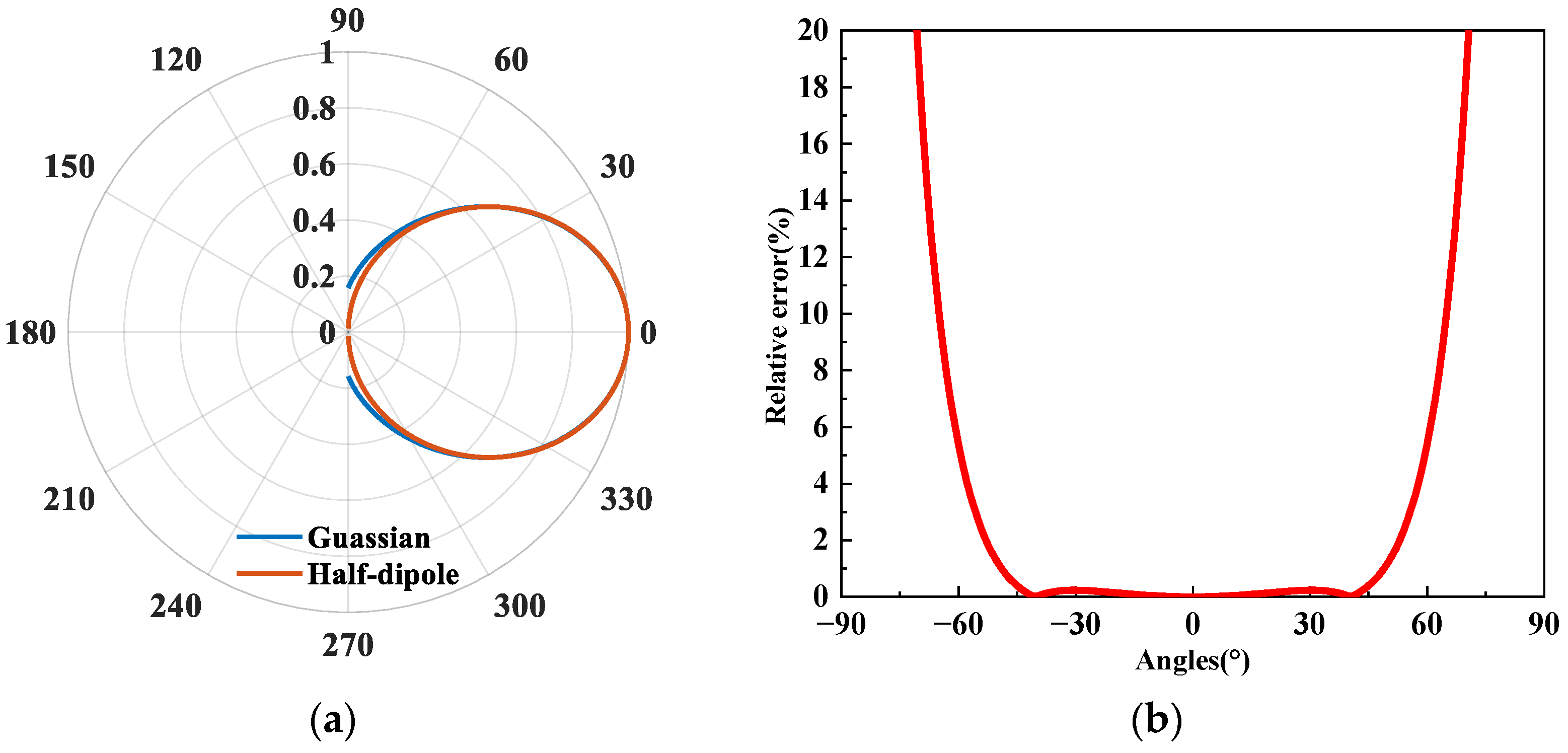
3.1. Antenna Pattern

The beamwidth of the half-wave dipole antenna is 78°, and the Gaussian simulation is also set with the same beamwidth. Figure 1a shows the comparison of far-field patterns between the Gaussian beam and the half-wave dipole antenna, while Figure 1b illustrates the relative error between the two beams. The results demonstrate that the far-field pattern function of the two beams accurately simulates the half-power beamwidth, with a relative error of less than 2%. As the radiation angle increases, the relative error between the two beams gradually increases. At a deviation of 60° from the main beam, the relative error reaches 5% and rapidly increases.

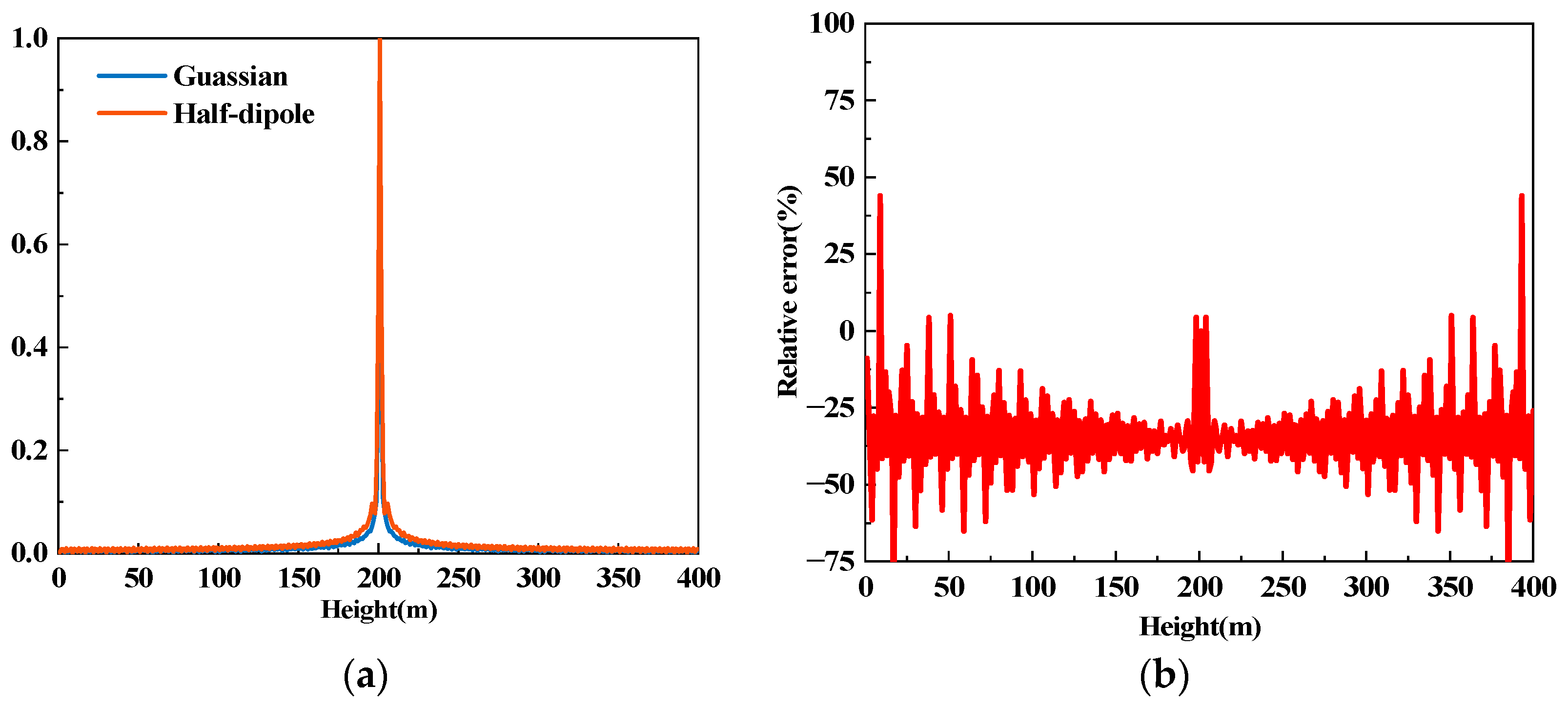
3.2. The Initial Field

The transmitting antenna is positioned at a 0-degree elevation angle with a height of 200 m, and the calculated vertical direction height is 400 m. The pattern functions of the two beams are substituted into Equations (11)–(14), resulting in two initial fields shown in Figure 2a and the corresponding relative errors depicted in Figure 2b.

As shown in Figure 2, when constructing the initial antenna field of the radio wave propagation model, using a Gaussian approximation to the actual wide beam to transmit the main beam of the antenna will result in certain relative errors, with the relative errors increasing as it moves away from the main beam. Figure 2b shows that the relative error near the height of the transmitting antenna is approximately 0%, whereas the relative error away from the height of the transmitting antenna is approximately 30%. The interference of the region above the surface causes the relative inaccuracy to fluctuate. The error of the initial field in PE modeling will result in a change in the calculation accuracy of the propagation loss in the coverage area of the radio wave propagation.

3.3. Propagation Loss Simulated with Wide-Angle PE Method

The PE simulation of space radio wave propagation loss is carried out by constructing the initial field with these two antennas. The radio wave propagation model theory in Section 2 is adopted to construct the propagation model. The specific algorithm construction process is as follows: (1) The Gaussian beam pattern and half-wave dipole antenna pattern are substituted into Equations (11)–(14) to calculate the initial field of the antenna; (2) The field distribution of the whole calculation domain is solved iteratively by Equation (8); (3) The Turkey absorption window in Equation (9) was used for the upper boundary processing of the calculation domain, and the impedance boundary conditions in Equation (10) were used for the underlying surface processing; (4) By substituting the field distribution of the entire computational domain into the propagation loss Equation (15) of the parabolic equation, the propagation loss value of the entire computational domain can be obtained.

The atmospheric environment used for calculation is the standard atmosphere, with the standard atmospheric refractive index profile. The underlying surface is flat soil with a relative dielectric constant of 4 and an electrical conductivity of 0.03. The calculation area covers the loss of space wave propagation within a horizontal distance of 10 km and a vertical distance of 400 m. The simulation calculation is focused on the regional radio station in Wuhan, operating at a radio frequency of 92.7 MHz. Figure 3a,b presents the calculation results of propagation loss within a vertical height of 400 m. The green solid line represents the Gaussian beam approximation result, while the red solid line represents the simulation calculation result of the half-wave dipole antenna.

Figure 3 shows that the obvious difference in the propagation loss of the two beams at 0.75 km is mainly concentrated in the main beam region. The electric field energy distribution using the Gaussian approximation is more dispersed and shows a larger propagation loss near the main beam. The average difference in the propagation loss of the two beams in the range of 150–250 m is 2.29 dB, and the average difference in the loss in other height ranges is 1.22 dB. The difference in propagation loss between the two beams at 10km is reduced, and the average difference in loss is 1.49 dB. The phenomenon of beam splitting is obvious, which reflects the inversely proportional change in radiation field energy and distance square. It also reflects the influence of the superposition of underlying surface-reflected waves in radio wave propagation.

4. Evaluation Based on Experimental Data

In this paper, an experimental system is built to measure the reception strength of FM radio signals. The experimental system can record the received power and the received position of the radio signal at a set frequency. A broadcast signal with a central frequency of 92.7 MHz was selected in Wuhan to conduct a propagation loss measurement experiment. The experiment was conducted on 5 November 2022. The atmospheric refractive index profile during the experiment is shown in Figure 4, and the underlying surface profile topography and propagation path are shown in Figure 5.

4.1. Radio Wave Propagation Simulation

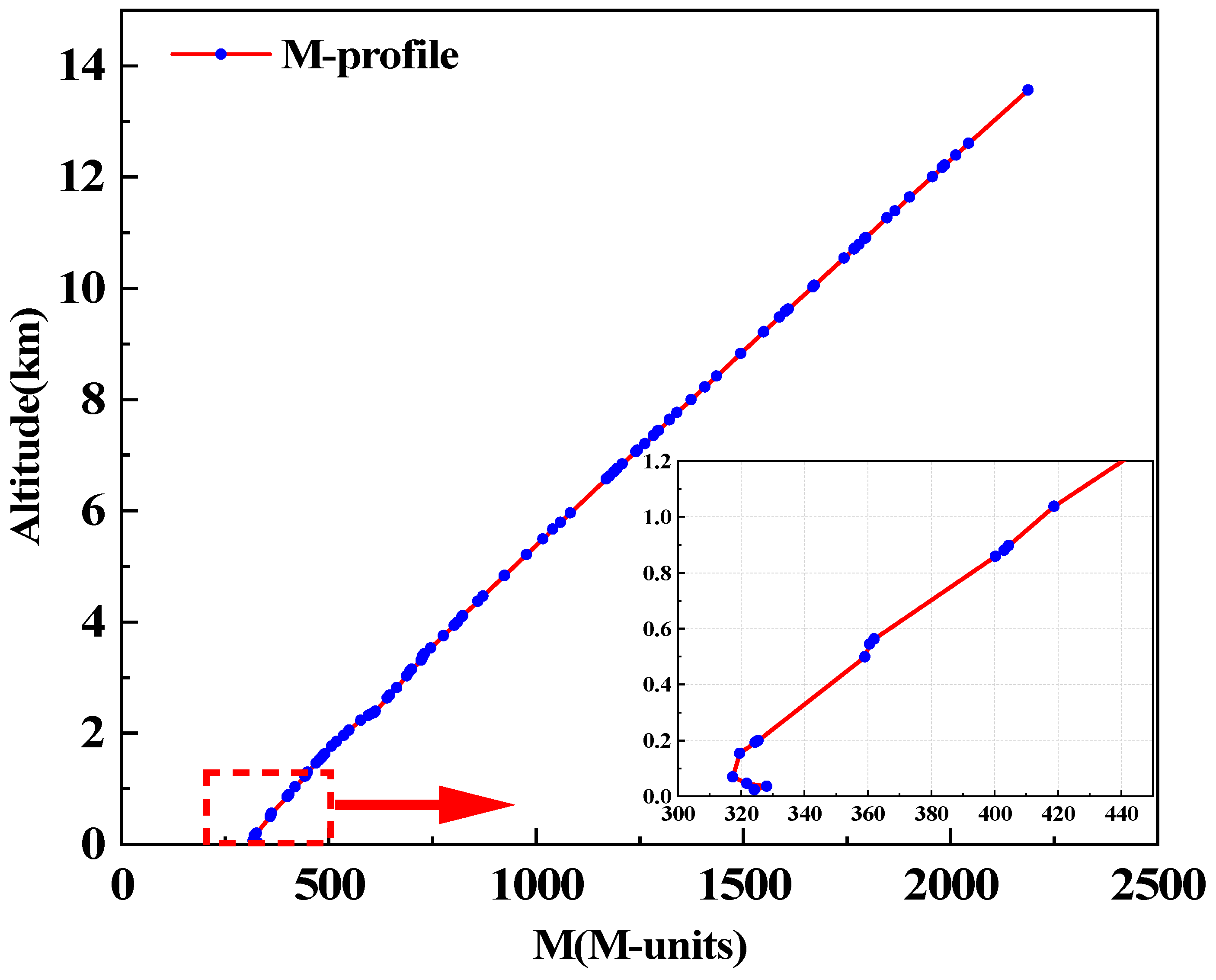
4.1.1. Atmospheric Structure

This article selects the temperature T (K), water vapor pressure $e$ (hPa), atmospheric pressure $P$ (hPa), and altitude $h$ (km) obtained from the Wuhan sounding station on the day of the measurement experiment to calculate the atmospheric refractive index profile. The equation is as follows:

$$N=\frac{77.6}{T}(P+4810\frac{e}{T})$$

(23)

$$M=N+157h$$

(24)

The water pressure $e$(hPa) is given by Equations (25) and (26):

$$e=\frac{H\cdot e_s}{100}$$

(25)

$$\begin{array}{l}{e}_s=EF\cdot a\cdot \exp [\frac{(b-\frac{t}{d})\cdot t}{t+c}]\\ E{F}_{water}=1+{10}^{-4}[7.2+P\cdot (0.00320+5.9\cdot {10}^{-7}\cdot t^2)]\\ E{F}_{ice}=1+{10}^{-4}[2.2+P\cdot (0.00382+6.4\cdot {10}^{-7}\cdot t^2)]\end{array}$$

(26)

$t$ is the dew point temperature (°C), and $e_s$ is the saturated water vapor pressure (hPa). When the dew point temperature is below zero, $a$ = 6.1115; $b$ = 23.036; $c$ = 279.82, and $d$ = 333.7. When the dew point temperature is above zero, $a$ = 6.1121; $b$ = 18.678; $c$ = 257.14, and $d$ = 234.5. According to Equations (23)–(26), the corrected atmospheric refractive index profile for the day is calculated as shown in Figure 4.

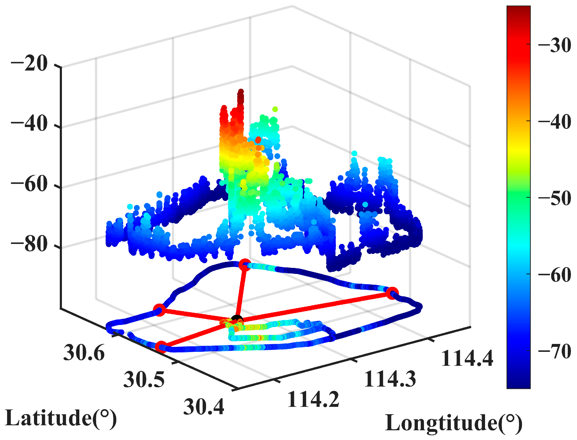
4.1.2. Underlying Surface Topographic Profile

In real propagation scenarios, radio wave propagation modeling needs to take into account the influence of the actual terrain. We have collected geographical information on the Wuhan area and extracted the topographic profile and other relevant information along the propagation path. Figure 5a shows the topographic map of Wuhan and the location information of measuring points in the signal measurement coverage area. Four different measuring points are selected from the experimental measurement path, and different radio wave propagation paths are obtained by connecting transmitting points and measuring points. The four paths include actual propagation scenarios, such as overwater surfaces and mountains. The topographic profile was obtained by meshing the four propagation paths, as shown in Figure 5b. The elevation data from different topographic profiles are analyzed to distinguish the underlying topographic features of each propagation path.

Table 1. Longitude and latitude information.

	Longitude (°)	Latitude (°)	Distance (km)
transmitter	114.2751	30.5580	0
point 1	114.2320	30.6318	9.19
point 2	114.3835	30.6835	17.39
point 3	114.1663	30.5440	10.54
point 4	114.4527	30.5267	17.36

shows the location information of the transmitting point and the measuring point, and the distance is the great circle distance between different measuring points and the transmitting point.

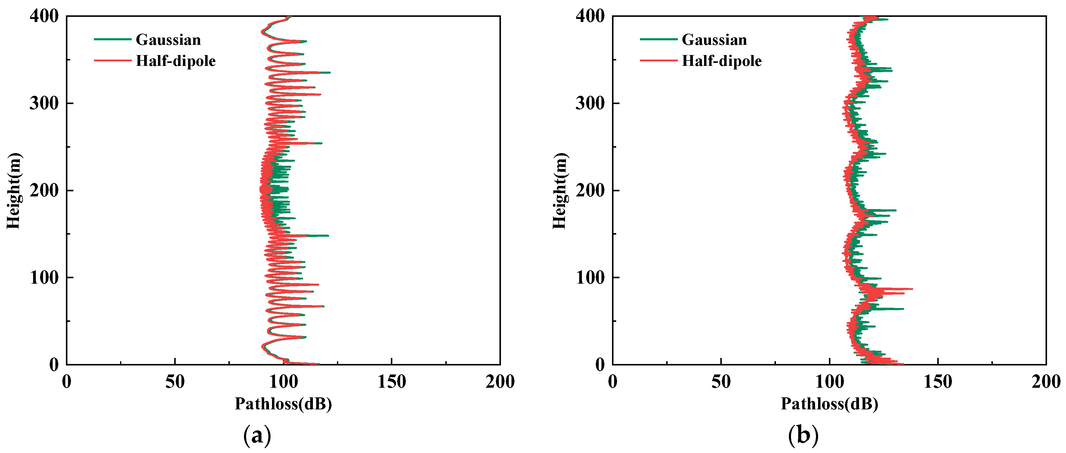
4.1.3. Propagation Loss Calculation Results

In the actual scene radio wave propagation modeling, this paper uses Gaussian beam approximation and the actual transmitting antenna pattern, respectively, to construct the broadcast signal propagation model. The modeling details are as follows: The actual atmospheric refractive index profile is constructed based on atmospheric environmental data during the experimental test. Combining the location information of test points and the radio wave coverage area, the topographic profile data on the propagation path are extracted to construct the underlying surface. In addition to the difference in the initial field construction, the other actual propagation environments of the two propagation models are consistent. The propagation losses on four large circle profile paths obtained using the wide-angle PE method are shown in Figure 6. It can be clearly observed that the impact of topographic occlusion on radio wave propagation loss and obvious clearance area will be generated after the mountain occlusion.

The real scenario wave propagation loss values calculated using the actual transmitting antenna directional pattern and Gaussian beam simulation are listed in

Table 2. Calculated propagation loss of half wave dipole measuring point.

Height (m)	Point 1 (dB)	Point 2 (dB)	Point 3 (dB)	Point 4 (dB)
1	129.0	136.7	134.2	149.9
2	132.1	132.5	134.8	147.0
3	125.6	128.2	125.3	147.7
4	120.0	130.6	119.2	145.5

and

Table 3. Calculated propagation loss of Gaussian beam measuring point.

Height (m)	Point 1 (dB)	Point 2 (dB)	Point 3 (dB)	Point 4 (dB)
1	126.3	131.3	130.1	148.6
2	133.8	128.0	126.6	147.5
3	124.5	125.5	122.7	151.8
4	119.1	124.6	116.7	147.5

. The two wave propagation models keep the same conditions except for the different directional pattern functions used in the construction of the initial antenna field.

The above two tables indicate that under identical calculation conditions, the radio wave propagation model constructed using the two-directional graph functions at varying heights exhibits maximum, minimum, and average differences of 8.15 dB, 0.49 dB, and 2.11 dB, respectively, at the same measuring point. The variation in loss among different propagation paths is influenced by the topographic complexity of each path.

4.2. Experimental Test Results of Radio Wave Propagation Loss

The received power on the measurement path is shown in Figure 7.

In Figure 7, the black dot represents the radiation source; the red dot represents the measurement point, and the red line represents the radio wave propagation path. The radiation source of this paper is Gui-shan Signal Tower in the Wuhan area, and its transmitting power is 10 kw; thus, the transmitting power is 70 dBm [22]. Considering the impact of small-scale fading, the distance between the measurement points for receiving power should fall within the range of 20 to 40 times the wavelength [23]. The experimental measuring vehicle maintains an average speed of 44.9 km/h, and the average data collected within a 6-s interval satisfy the requirements for data processing. The average received power at the four measuring points is −64 dBm, −71.2 dBm, −65.5 dBm, and −72.9 dBm, resulting in real propagation losses of 134.0 dB, 141.2 dB, 135.5 dB, and 142.9 dB, respectively.

4.3. Differential Analysis

The receiving antenna is positioned 1 m above the ground surface, and the loss value at this height is used as the calculated predicted loss for radio wave propagation.

Table 4. Comparison of loss at measuring points of the two models.

Point	Gaussian (dB)	Half-Wave (dB)	Measured Value (dB)	Terrain Mean Height (m)
1	126.3	129.0	134.0	16.14
2	131.3	136.7	141.2	5.13
3	130.1	134.2	135.5	19.61
4	148.6	149.9	142.9	22.94

presents a comparison between the predicted loss value of the radio wave propagation model and the measured data.

Table 4 shows that the predicted loss of the broadcast signal propagation model, based on the half-wave dipole antenna, is closer to the actual measured value for measuring points 1–3, while the propagation loss at measuring point 4 is significantly increased due to the clear topographic obstruction at the receiving position. The average measured loss for the four measurement points is 138.4 dB. The average predicted loss of the model based on the half-wave dipole antenna is 137.5 dB, with a loss correlation coefficient of 0.873 between the simulated calculation and the measured data. On the other hand, the average loss predicted by the model based on Gaussian simulation is 134.1 dB, with a loss correlation coefficient of 0.805 between the simulation and the measured data. From the above comparison, it is evident that the radio wave propagation model based on the actual transmitting antenna pattern exhibits better prediction accuracy.

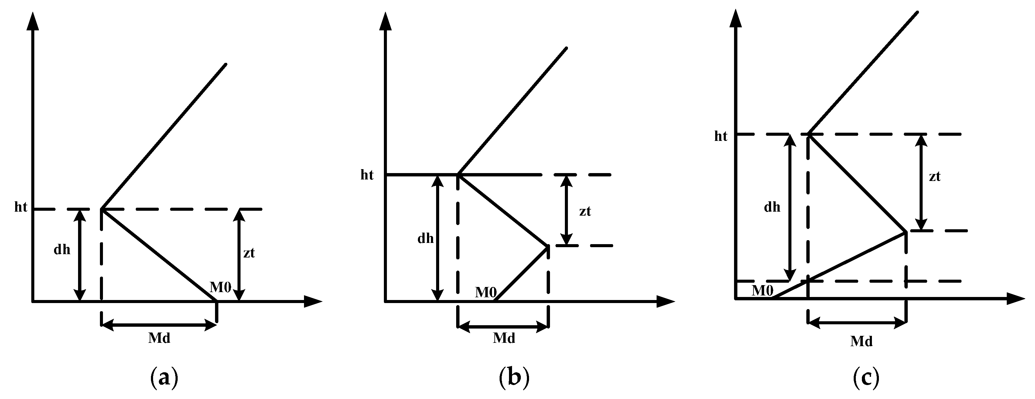
5. Inversion of Atmospheric Refractive Index Profile

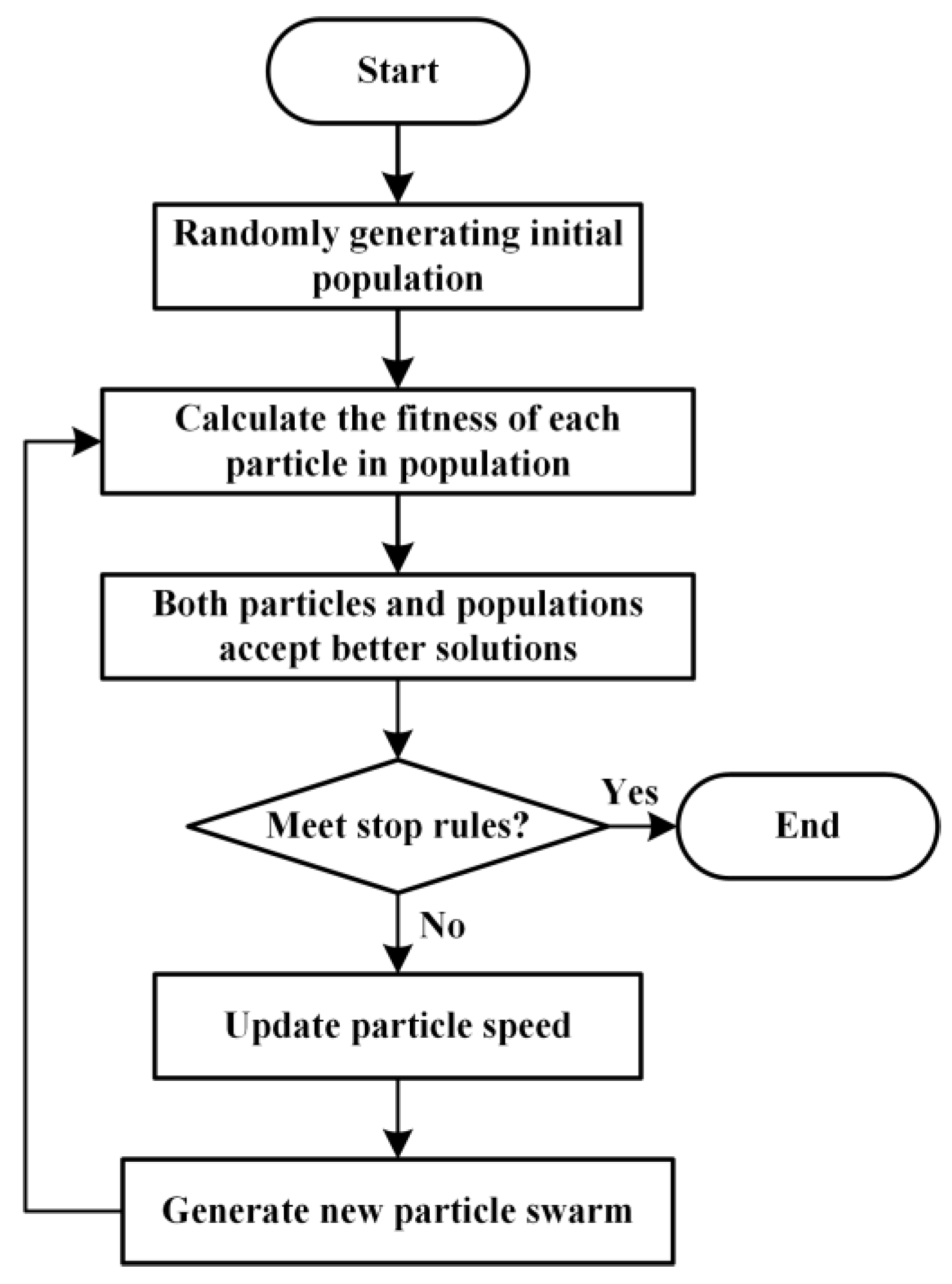
5.1. Inversion Algorithm

To assess the accuracy of the inversion of atmospheric refractive index profiles using the radio wave propagation models based on the two initial fields, particle swarm optimization (PSO) is employed to determine the atmospheric environment parameters for each model. The inversion path corresponds to measurement path 3. Figure 8 illustrates the flow chart of the particle swarm optimization algorithm, while

Table 5. Parameters of PSO algorithm.

Parameter	Value
Maximum number of iterations	50
Number of particles	100
Individual learning factor	1
Social learning factor	1
Maximum inertia factor	0.9
Minimum inertia factor	0.4

presents the algorithm’s parameters.

Tropospheric duct structure is a common atmospheric refractive index profile structure. Figure 9 shows the modified refractive index profiles corresponding to different types of lower atmospheric ducts.

In Figure 9, $h_t$ is the duct top height in meters; $dh$ is the duct thickness in meters; $M_0$ is the modified surficial refractivity in M units; $M_d$ is the duct strength in M units, and $z_t$ is the duct layer thickness in meters. The atmospheric refractive index profile on the day of the experimental test is shown in Figure 4, which conforms to the ground-attached duct (including the base layer) structure in the atmospheric duct structure and is further simplified, as shown in Figure 9b.

5.2. Inversion Results Analysis

The inversion results of the two models and the actual parameters are shown in

Table 6. Comparison of inversion parameters of two models based on PSO algorithm.

Parameter	Gaussian	Half-Wave	Actual Atmospheric Parameter
$M_0$ (M-units)	320.4	323.3	324
$M_d$ (M-units)	10	12	14
$dh$ (m)	85.1	84.8	82
$z_t$ (m)	52.4	49.5	47
$h_t$ (m)	85.1	84.8	82

.

In Table 6, the root-mean-square error (RMSE) of Gaussian beam approximation is 3.85, and the half-wave mode is 2.03. The propagation model based on the actual transmitting antenna pattern is closer to the measured duct parameters under the same inversion algorithm. The more accurate the radio wave propagation model is, the higher the accuracy of atmospheric environment inversion using this model.

6. Conclusions

This paper analyzed the disparity between the Gaussian beam simulation and the actual antenna pattern in constructing the initial field of the parabolic equation and investigated its impact on the propagation loss of the radio wave model. Based on the simulation results of radio wave propagation and the analysis of measured data of broadcast signals in the Wuhan area, the findings indicate that the broadcast signal propagation model, which incorporates the actual antenna pattern, aligns more closely with the actual spatial propagation characteristics of radio waves, with a correlation coefficient of 0.873. Lastly, particle swarm optimization is employed to invert the tropospheric refractive index profile of radio wave propagation. The results demonstrate that the model utilizing the actual transmitting antenna pattern achieves higher inversion accuracy, with a root-mean-square error of 2.03.

In conclusion, to enhance the accuracy of the wave propagation model for wide-beam transmitting antennas, it is recommended to construct the initial field of the parabolic equation based on the actual antenna pattern instead of simulating the transmitting antenna using the Gaussian beam. Additionally, considering the interdependence among tropospheric duct parameters [2], historical atmospheric environment information can be statistically analyzed to optimize the multi-parameter variation range of the inversion algorithm and improve its accuracy and efficiency.

References

1. Levy, M.F. Diffraction Studies in Urban Environment with Wide-Angle Parabolic Equation Method. Electron. Lett. 1992, 28, 1491–1492. [Google Scholar] [CrossRef]
2. Liu, C.G.; Zhou, H.K.; Hu, W.T.; Duan, K.; Cheng, R.; Huang, L.; Guo, X.; Wang, H.; Cai, H. An inversion method of anomalous atmospheric refractive environment. Chin. J. Radio Sci. 2022, 37, 222–228. (In Chinese) [Google Scholar]
3. Hardin, R.H.; Tappert, F.D. Applications of the Split-Step Fourier Method to the Numerical Solution of Nonlinear and Variable Coefficient Wave Equations. SIAM Rev. Chron. 1973, 15, 423. [Google Scholar]
4. Claerbout, J.F. Fundamentals of Geophysical Data Processing with Application to Petroleum Prospect; McGraw-Hill Press: New York, NY, USA, 1976. [Google Scholar]
5. Feit, M.D.; Fleck, J.A. Light Propagation in Graded-Index Optical Fibers. Appl. Opt. 1978, 17, 3990–3998. [Google Scholar] [CrossRef] [PubMed]
6. Thomson, D.J.; Chapman, N.R. A Wide-Angle Split-Step Algorithm for the Parabolic Equation. J. Acoust. Soc. Am. 1983, 74, 1848–1854. [Google Scholar] [CrossRef]
7. Greene, R.R. The rational approximation to the acoustic wave equation with bottom interaction. J. Acoust. Soc. Am. 1984, 76, 1764–1773. [Google Scholar] [CrossRef]
8. Levy, M.F. Parabolic Equation Methods for Electromagnetic Wave Propagation; Institution of Electrical Engineers: London, UK, 2000; pp. 40–41. [Google Scholar]
9. Rao, B.; Carin, L. A Hybrid (Parabolic Equation)-(Gaussian Beam) Algorithm for Wave Propagation through Large Inhomogeneous regions. IEEE Trans. Antennas Propag. 1998, 46, 700–709. [Google Scholar]
10. Zhang, X.; Sarris, C.D. A Gaussian Beam Approximation Approach for Embedding Antennas into Vector Parabolic Equation-Based Wireless Channel Propagation Models. IEEE Trans. Antennas Propag. 2017, 65, 1301–1310. [Google Scholar] [CrossRef]
11. L’Hour, C.A.; Fabbro, V.; Chabory, A.; Sokoloff, J. 2-D Propagation Modeling in Inhomogeneous Refractive Atmosphere Based on Gaussian Beams Part II: Application to Radio Occultation. IEEE Trans. Antennas Propag. 2019, 67, 5487–5496. [Google Scholar] [CrossRef]
12. Goldsmith, P.F. Quasioptical Systems: Gaussian Beam Quasioptical Propagation and Applications; IEEE Press: Piscataway, NJ, USA, 1998. [Google Scholar]
13. Trappe, N.; Murphy, J.A.; Withington, S. The Gaussian Beam Mode Analysis of Classical Phase Aberrations in Diffraction-Limited Optical Systems. Eur. J. Phys. 2003, 24, 403–412. [Google Scholar] [CrossRef]
14. Xiong, W.; Hu, J.; Zhong, K.; Sun, Y.; Xiao, X.; Zhu, G. MIMO Radar Transmit Waveform Design for Beampattern Matching via Complex Circle Optimization. Remote Sens. 2023, 15, 633. [Google Scholar] [CrossRef]
15. Apaydin, G.; Sevgi, L. Groundwave Propagation at Short Ranges and Accurate Source Modeling. IEEE Antennas Propag. Mag. 2013, 55, 244–262. [Google Scholar] [CrossRef]
16. Li, Y.; Liu, C.G.; Zhong, M.; Wang, Y.; Yang, M. Radio Wave Propagation Path Loss in the Irregular Terrain environments. In Proceedings of the 2009 3rd IEEE International Symposium on Microwave, Antenna, Propagation and EMC Technologies for Wireless Communications, Beijing, China, 27–29 October 2009; pp. 627–630. [Google Scholar]
17. Harris, F.J. On the Use of Windows for Harmonic Analysis with the Discrete Fourier Transform. Proc. IEEE 1978, 66, 51–83. [Google Scholar] [CrossRef]
18. Kuttler, J.R.; Huffaker, J.D. Solving the Parabolic Wave Equation with a Rough Surface Boundary Condition. J. Acoust. Soc. Am. 1993, 94, 2451–2453. [Google Scholar] [CrossRef]
19. Hu, H.B.; Mao, J.J.; Cai, S.L. Green’s Function of Wide-angle Parabolic Equation and Its Applications. J. Electron. 2006, 34, 517–521. (In Chinese) [Google Scholar]
20. Wu, Z.Z. Mobile Communication Radio Wave Propagation; People’s Posts and Telecommunications Publishing House: Beijing, China, 2002. (In Chinese) [Google Scholar]
21. Barrios, A.E. A terrain parabolic equation model for propagation in the troposphere. IEEE Trans. Antennas Propag. 1994, 42, 90–98. [Google Scholar] [CrossRef]
22. Hu, W.T.; Liu, C.G.; Lin, F.J.; Zhang, Y.S.; Guo, X.M. Characteristics of atmospheric ducts and its impact on FM broadcasting. J. Radio Sci. 2020, 35, 856–867. (In Chinese) [Google Scholar]
23. Dupleich, D.; Müller, R.; Landmann, M.; Shinwasusin, E.A.; Saito, K.; Takada, J.I.; Luo, J.; Thomä, R.; Del Galdo, G. Multi-Band Propagation and Radio Channel Characterization in Street Canyon Scenarios for 5G and Beyond. IEEE Access 2019, 7, 160385–160396. [Google Scholar] [CrossRef]
Figure 1. Comparison of far-field pattern of two beams. (a) Far-field pattern comparison; (b) Relative error between beams.
Atmosphere 15 00046 g001
Figure 2. Initial field comparison of two beams. (a) Initial field comparison. (b) Relative error between beams.
Atmosphere 15 00046 g002
Figure 3. Calculation of radio wave propagation loss under ideal conditions. (a) Propagation loss at 0.75 km. (b) Propagation loss at 10 km.
Atmosphere 15 00046 g003
Figure 4. Modified atmospheric refraction profile.
Atmosphere 15 00046 g004
Figure 5. Actual terrain processing. (a) Location map of measuring points. (b) Path topographic profile.
Atmosphere 15 00046 g005
Figure 6. Distribution of propagation loss in different paths. (a) Path 1 propagation loss. (b) Path 2 propagation loss. (c) Path 3 propagation loss. (d) Path 4 propagation loss.
Atmosphere 15 00046 g006
Figure 7. The received power position diagram on the measurement path.
Atmosphere 15 00046 g007
Figure 8. Basic flowchart of PSO algorithm.
Atmosphere 15 00046 g008
Figure 9. Different types of lower atmospheric ducts. (a) Surface duct. (b) Surface-based duct. (c) Elevated duct.
Atmosphere 15 00046 g009