
Application of CFD Modelling for Pollutant Dispersion at an Urban Traffic Hotspot


Abstract
1. Introduction
2. Methodology
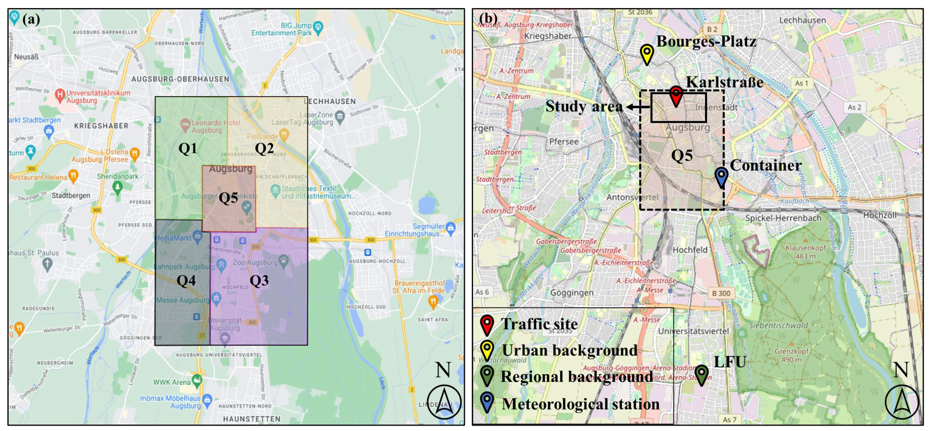
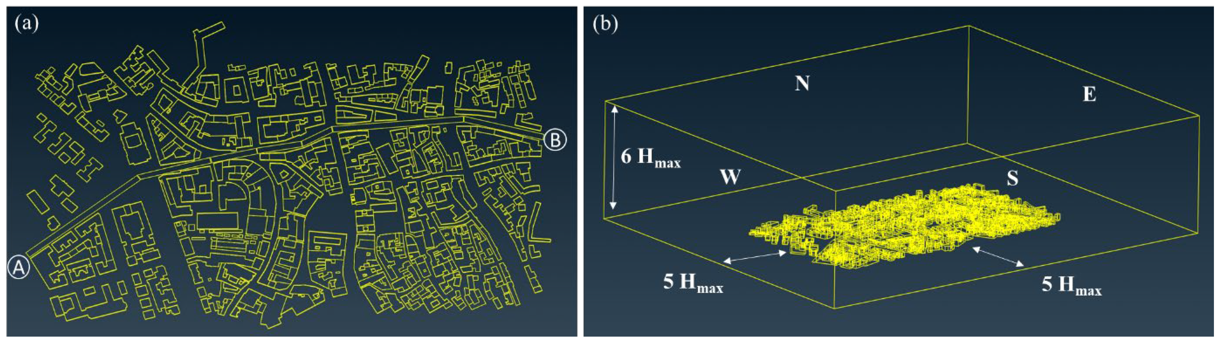
2.1. Area of Interest and Geometrical Model
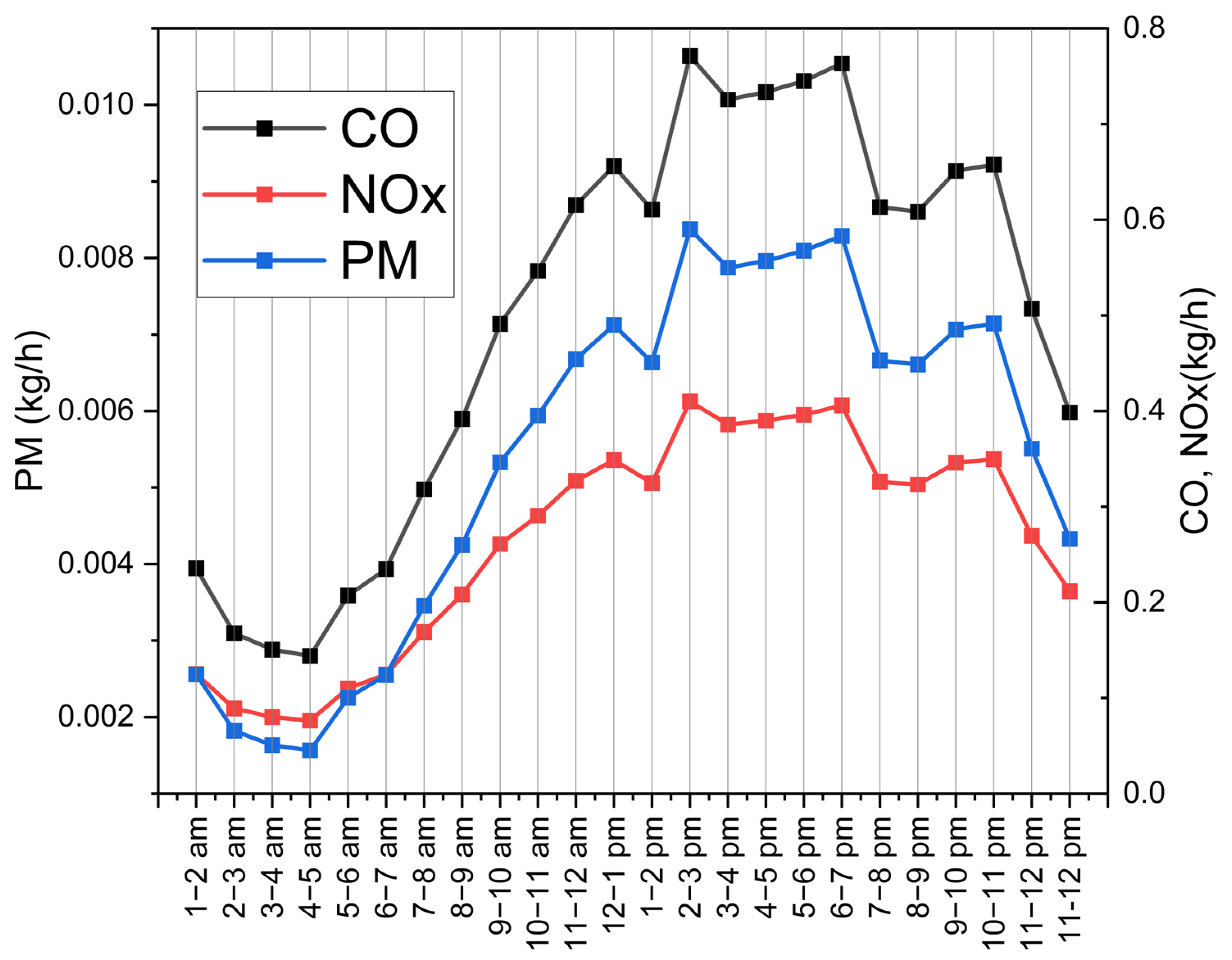
2.2. Traffic Emissions
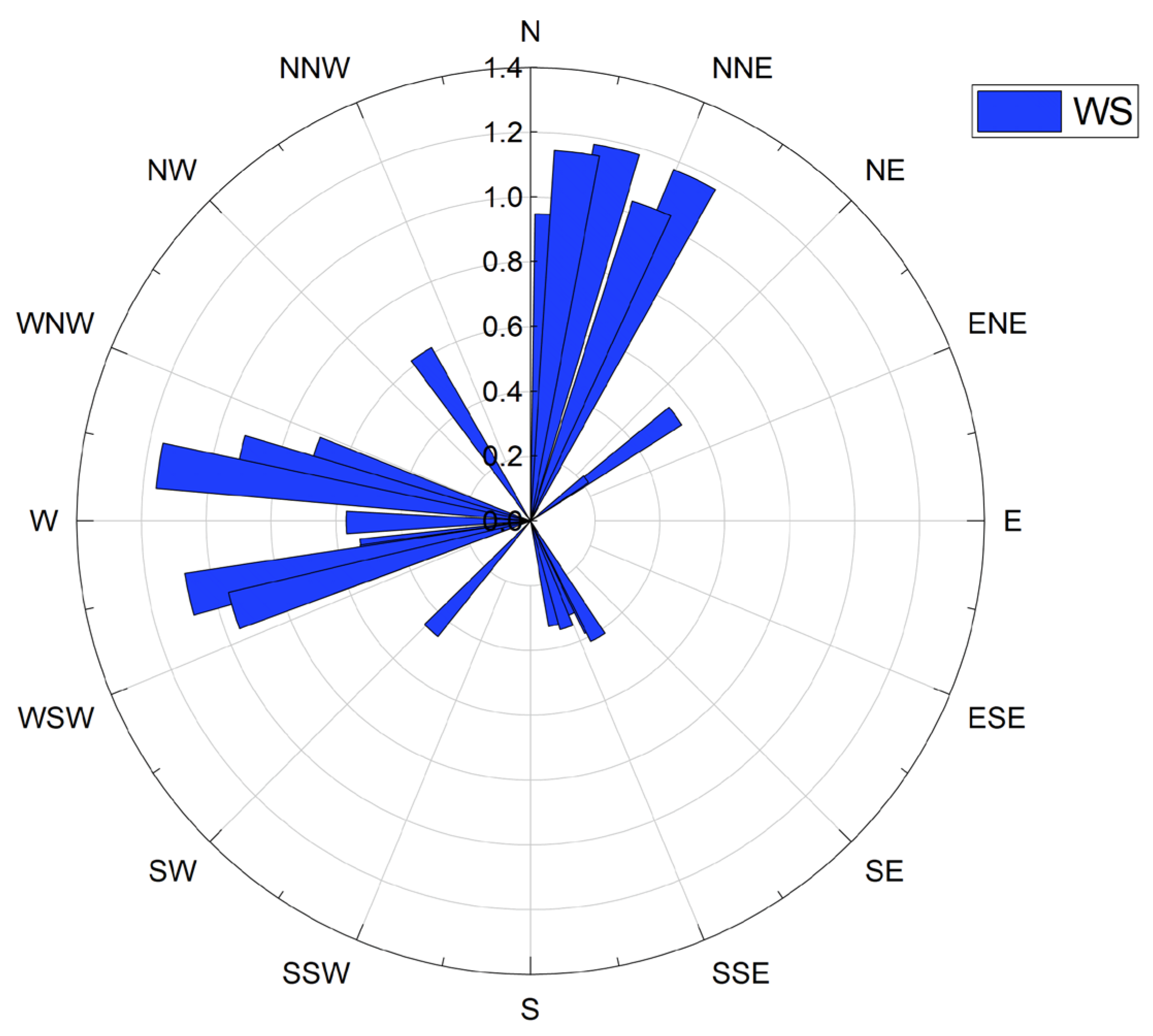
2.3. Meteorological Conditions
2.4. CFD Model Setup
2.4.1. Numerical Model
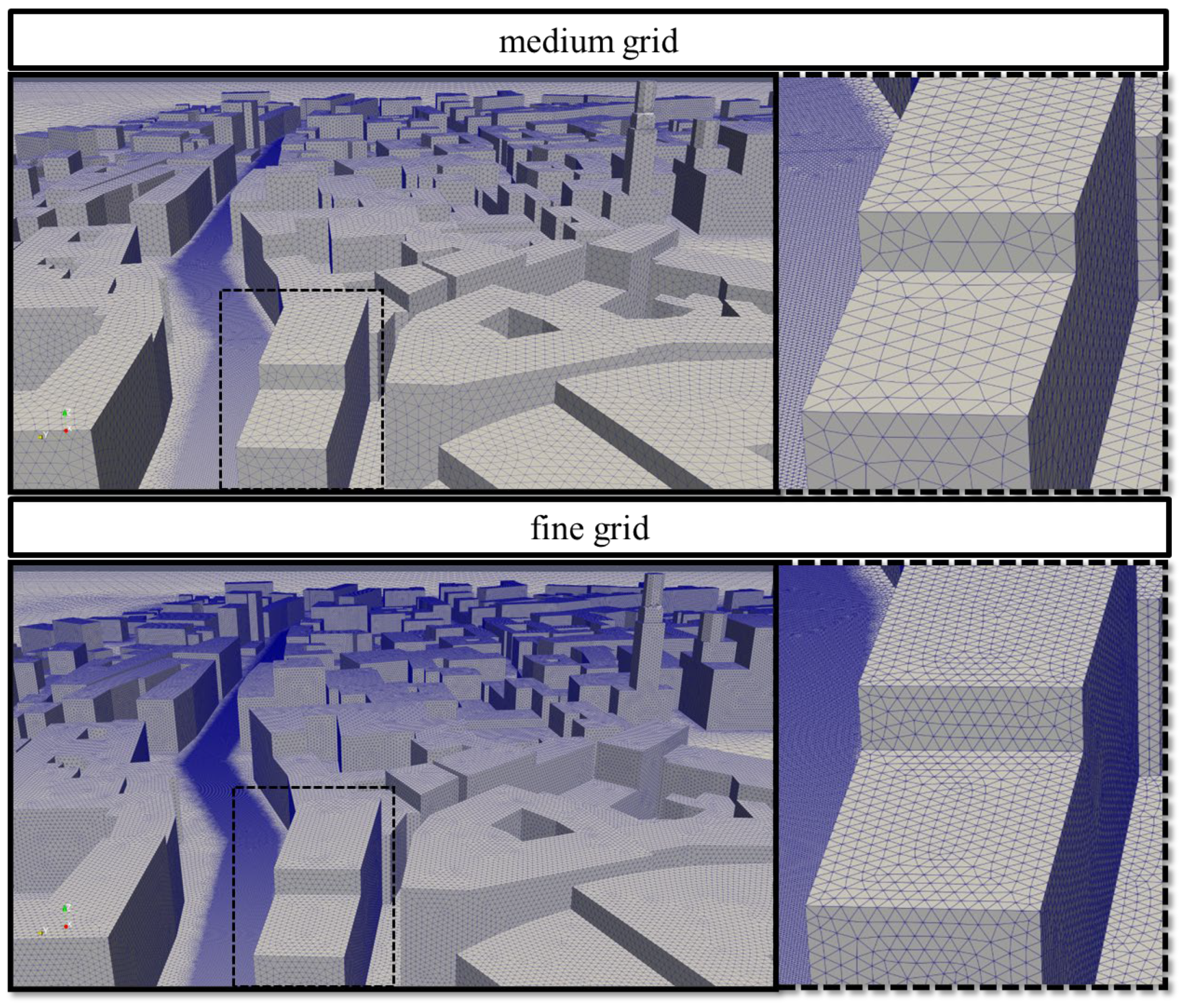
2.4.2. Computational Mesh
3. Results
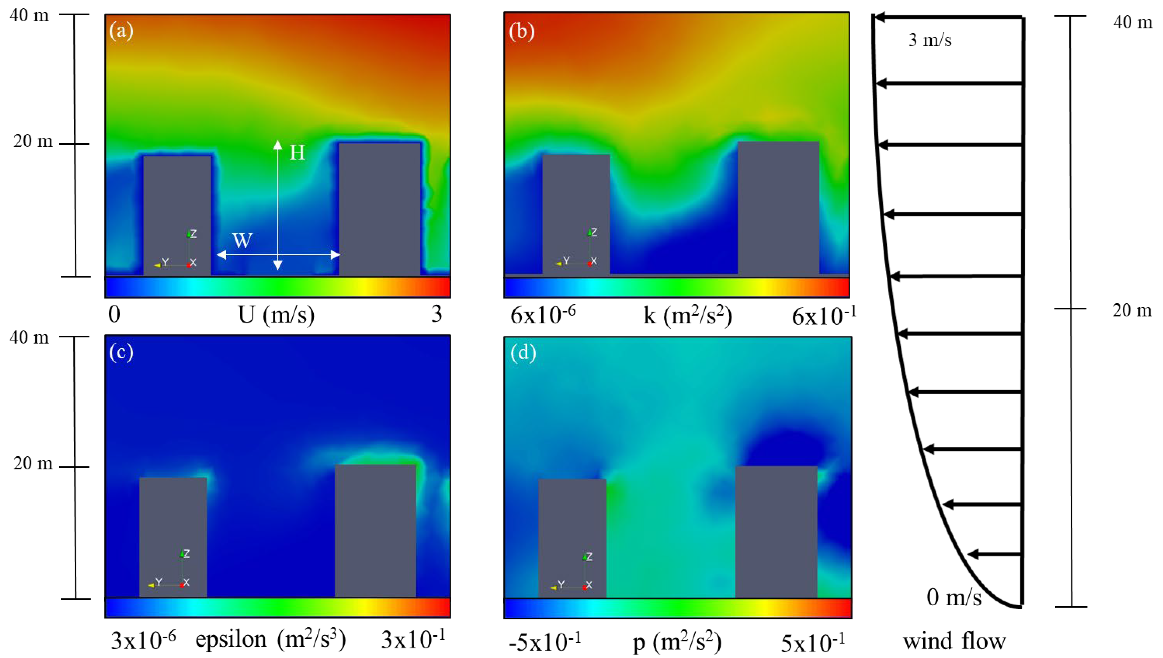
3.1. CFD Parameters
3.2. Pollutant Concentration at the Area of Interest
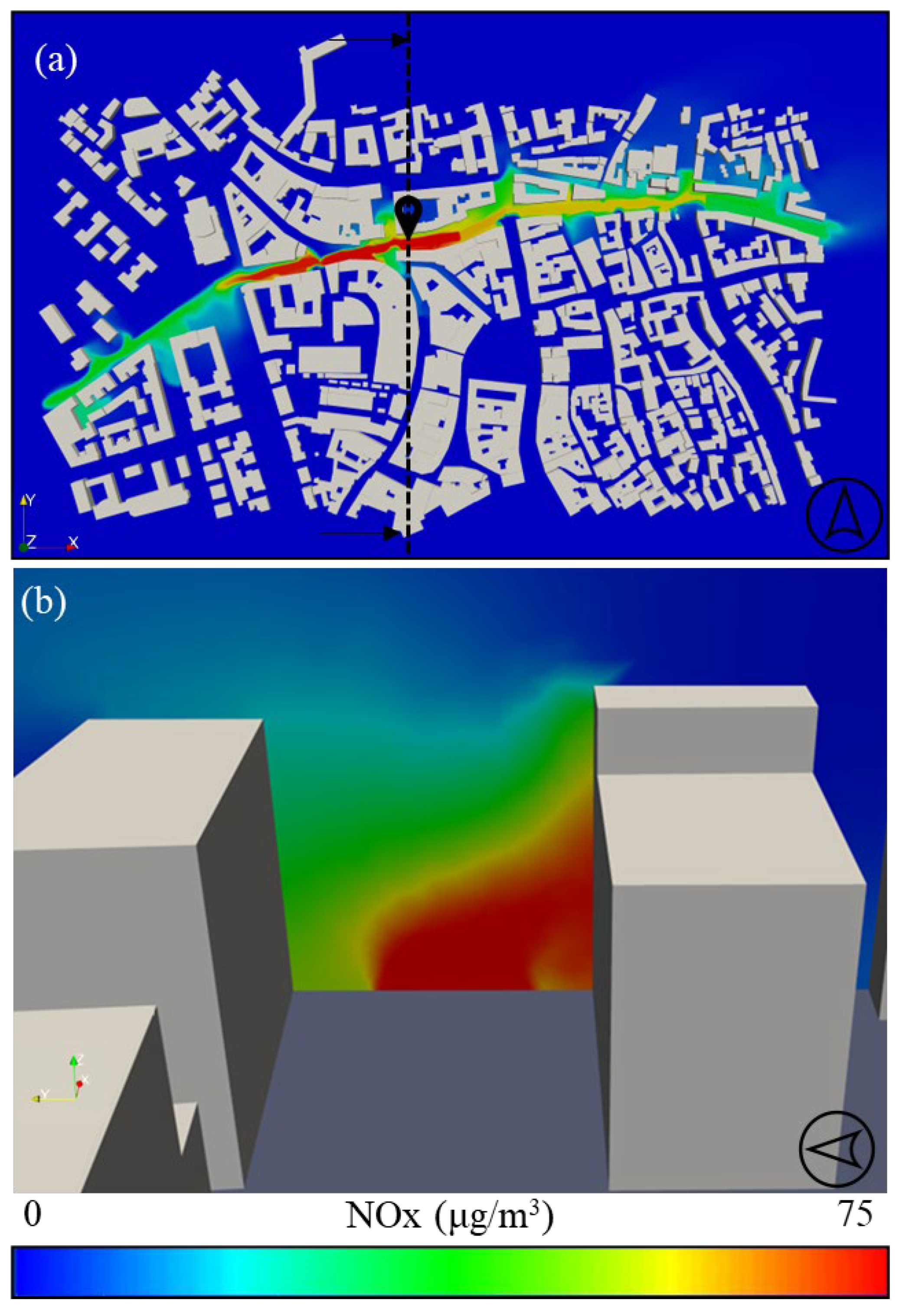
Pollutant Spatial Distribution
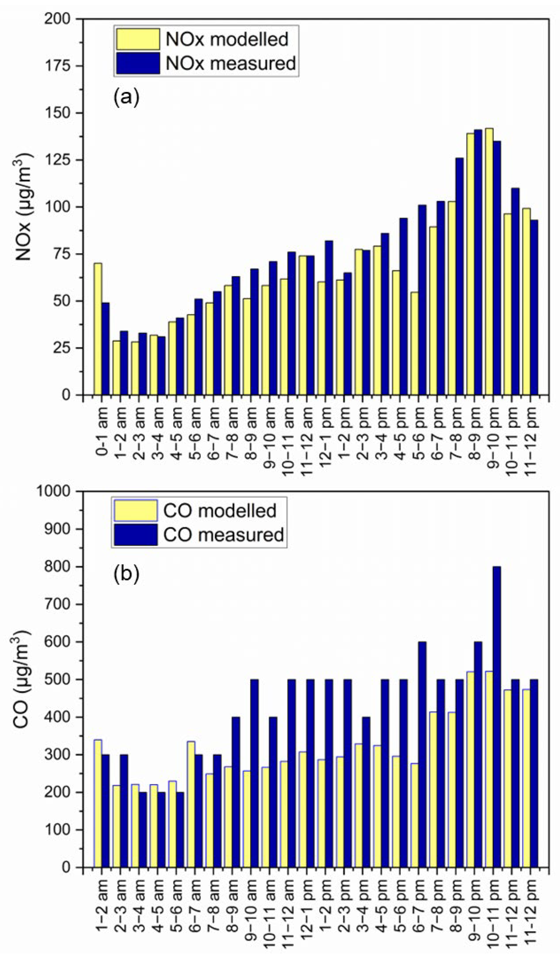
3.3. Daily Cycle and Comparison with Measurements
3.4. Validation Metrics for CFD Models
4. Conclusions
Author Contributions
Funding
Institutional Review Board Statement
Informed Consent Statement
Data Availability Statement
Acknowledgments
Conflicts of Interest
References
- Zhang, K.; Batterman, S. Air pollution and health risks due to vehicle traffic. Sci. Total Environ. 2013, 450–451, 307–316. [Google Scholar] [CrossRef] [PubMed]
- Ju, K.; Lu, L.; Wang, W.; Chen, T.; Yang, C.; Zhang, E.; Xu, Z.; Li, S.; Song, J.; Pan, J.; et al. Causal effects of air pollution on mental health among Adults—An exploration of susceptible populations and role of physical activity based on a longitudinal nationwide cohort in China. Environ. Res. 2022, 217, 114761. [Google Scholar] [CrossRef] [PubMed]
- Reşitoʇlu, I.A.; Altinişik, K.; Keskin, A. The pollutant emissions from diesel-engine vehicles and exhaust aftertreatment systems. Clean Technol. Environ. Policy 2015, 17, 15–27. [Google Scholar] [CrossRef]
- Li, F.; Schnelle-Kreis, J.; Cyrys, J.; Karg, E.; Gu, J.; Abbaszade, G.; Orasche, J.; Peters, A.; Zimmermann, R. Organic speciation of ambient quasi-ultrafine particulate matter (PM0.36) in Augsburg, Germany: Seasonal variability and source apportionment. Sci. Total Environ. 2018, 615, 828–837. [Google Scholar] [CrossRef] [PubMed]
- Angatha, R.K.; Mehar, A. Impact of Traffic on Carbon Monoxide Concentrations Near Urban Road Mid-Blocks. J. Inst. Eng. Ser. A 2020, 101, 713–722. [Google Scholar] [CrossRef]
- Grewe, V.; Dahlmann, K.; Matthes, S.; Steinbrecht, W. Attributing ozone to NOx emissions: Implications for climate mitigation measures. Atmos. Environ. 2012, 59, 102–107. [Google Scholar] [CrossRef]
- Chen, R.; Pan, G.; Zhang, Y.; Xu, Q.; Zeng, G.; Xu, X.; Chen, B.; Kan, H. Ambient carbon monoxide and daily mortality in three Chinese cities: The China Air Pollution and Health Effects Study (CAPES). Sci. Total Environ. 2011, 409, 4923–4928. [Google Scholar] [CrossRef]
- Yazid AW, M.; Sidik nor, A.C.; Salim, S.M.; Saqr, K.M. A review on the flow structure and pollutant dispersion in urban street canyons for urban planning strategies. Simulation 2014, 90, 892–916. [Google Scholar] [CrossRef]
- Tee, C.; Ng, K.E.Y.; Xu, G. Analysis of transport methodologies for pollutant dispersion modelling in urban environments. J. Environ. Chem. Eng. 2020, 8, 103937. [Google Scholar] [CrossRef]
- Montazeri, H.; Blocken, B. CFD simulation of wind-induced pressure coefficients on buildings with and without balconies: Validation and sensitivity analysis. Build. Environ. 2013, 60, 137–149. [Google Scholar] [CrossRef]
- Su, J.; Wang, L.; Gu, Z.; Song, M.; Cao, Z. Effects of real trees and their structure on pollutant dispersion and flow field in an idealized street canyon. Atmos. Pollut. Res. 2019, 10, 1699–1710. [Google Scholar] [CrossRef]
- Fernández-Pacheco, V.M.; Álvarez-Álvarez, E.; Blanco-Marigorta, E.; Ackermann, T. CFD model to study PM 10 dispersion in large-scale open spaces. Sci. Rep. 2023, 13, 5966. [Google Scholar] [CrossRef]
- Toscano, D.; Marro, M.; Mele, B.; Murena, F.; Salizzoni, P. Assessment of the impact of gaseous ship emissions in ports using physical and numerical models: The case of Naples. Build. Environ. 2021, 196, 107812. [Google Scholar] [CrossRef]
- Sonia Oppo, W.; Karl, M.; Boikos, C.; Otto Paul, M. (Eds.) THE SCIPPER Project Shipping Contributions to Inland Pollution Push for the Enforcement of Regulations Deliverable Title Shipping Emissions Contribution to Port and Neighbouring Urban Areas Dissemination Level (*) Public (PU); Helmholtz-Zentrum Hereon: Geesthacht, Germany, 2023. [Google Scholar]
- Lauriks, T.; Longo, R.; Baetens, D.; Derudi, M.; Parente, A.; Bellemans, A.; van Beeck, J.; Denys, S. Application of Improved CFD Modeling for Prediction and Mitigation of Traffic-Related Air Pollution Hotspots in a Realistic Urban Street. Atmos. Environ. 2021, 246, 118127. [Google Scholar] [CrossRef]
- Sanchez, B.; Santiago, J.L.; Martilli, A.; Martin, F.; Borge, R.; Quaassdorff, C.; de la Paz, D. Modelling NOX concentrations through CFD-RANS in an urban hot-spot using high resolution traffic emissions and meteorology from a mesoscale model. Atmos. Environ. 2017, 163, 155–165. [Google Scholar] [CrossRef]
- Rivas, E.; Santiago, J.L.; Lechón, Y.; Martín, F.; Ariño, A.; Pons, J.J.; Santamaría, J.M. CFD modelling of air quality in Pamplona City (Spain): Assessment, stations spatial representativeness and health impacts valuation. Sci. Total Environ. 2019, 649, 1362–1380. [Google Scholar] [CrossRef] [PubMed]
- Akhatova, A.; Kassymov, A.; Kazmaganbetova, M.; Rojas-Solórzano, L. CFD Simulation of the Dispersion of Exhaust Gases in a Traffic Loaded Street of Astana, Kazakhstan. J. Urban Environ. Eng. 2015, 9, 158–167. [Google Scholar] [CrossRef]
- Blocken, B. Computational Fluid Dynamics for urban physics: Importance, scales, possibilities, limitations and ten tips and tricks towards accurate and reliable simulations. Build. Environ. 2015, 91, 219–245. [Google Scholar] [CrossRef]
- Zheng, X.; Montazeri, H.; Blocken, B. Large-eddy simulation of pollutant dispersion in generic urban street canyons: Guidelines for domain size. J. Wind Eng. Ind. Aerodyn. 2021, 211, 104527. [Google Scholar] [CrossRef]
- Tominaga, Y.; Mochida, A.; Yoshie, R.; Kataoka, H.; Nozu, T.; Yoshikawa, M.; Shirasawa, T. AIJ guidelines for practical applications of CFD to pedestrian wind environment around buildings. J. Wind Eng. Ind. Aerodyn. 2008, 96, 1749–1761. [Google Scholar] [CrossRef]
- Pantusheva, M.; Mitkov, R.; Hristov, P.O.; Petrova-Antonova, D. Air Pollution Dispersion Modelling in Urban Environment Using CFD: A Systematic Review. Atmosphere 2022, 13, 1640. [Google Scholar] [CrossRef]
- Naiudomthum, S.; Winijkul, E.; Sirisubtawee, S. Near Real-Time Spatial and Temporal Distribution of Traffic Emissions in Bangkok Using Google Maps Application Program Interface. Atmosphere 2022, 13, 1803. [Google Scholar] [CrossRef]
- Holmes, N.S.; Morawska, L. A review of dispersion modelling and its application to the dispersion of particles: An overview of different dispersion models available. Atmos. Environ. 2006, 40, 5902–5928. [Google Scholar] [CrossRef]
- Kowalski, M.; Hank, M.; Kusch, T.; Cyrys, J. Smart Air Quality Network-Network Planning Phase 1/2 Deployment of Scientific Scouts (EDM80NEPH, GRIMM) and Reference Devices OPC (EDM164, GRIMM) Augsburg, Bayern. 2018. Available online: https://www.smartaq.net/ (accessed on 19 October 2021).
- Jon, K.S.; Huang, Y.-D.; Sin, C.H.; Cui, P.-Y.; Luo, Y. Influence of wind direction on the ventilation and pollutant dispersion in different 3D street canyon configurations: Numerical simulation and wind-tunnel experiment. Environ. Sci. Pollut. Res. 2023, 30, 31647–31675. [Google Scholar] [CrossRef] [PubMed]
- Peralta, C.; Nugusse, H.; Kokilavani, S.P.; Schmidt, J.; Stoevesandt, B. Validation of the simpleFoam (RANS) solver for the atmospheric boundary layer in complex terrain. ITM Web Conf. 2014, 2, 01002. [Google Scholar] [CrossRef]
- Elfverson, D.; Lejon, C. Use and scalability of openfoam for wind fields and pollution dispersion with building-and ground-resolving topography. Atmosphere 2021, 12, 1124. [Google Scholar] [CrossRef]
- Miao, Y.; Liu, S.; Zheng, Y.; Wang, S.; Li, Y. Numerical study of traffic pollutant dispersion within different street canyon configurations. Adv. Meteorol. 2014, 2014, 458671. [Google Scholar] [CrossRef]
- Rapkos, N.; Weigelt, A.; Beecken, J.; Ntziachristos, L. Method to identify fuel sulphur content (FSC) violations of ongoing vessels using CFD modelling. Atmos. Environ. 2023, 309, 119912. [Google Scholar] [CrossRef]
- Bonifacio, H.F.; Maghirang, R.G.; Glasgow, L.A. Numerical simulation of transport of particles emitted from ground-level area source using AERMOD and CFD. Eng. Appl. Comput. Fluid Mech. 2014, 8, 488–502. [Google Scholar] [CrossRef]
- Tominaga, Y.; Stathopoulos, T. Turbulent Schmidt numbers for CFD analysis with various types of flowfield. Atmos. Environ. 2007, 41, 8091–8099. [Google Scholar] [CrossRef]
- Amorim, J.H.; Rodrigues, V.; Tavares, R.; Valente, J.; Borrego, C. CFD modelling of the aerodynamic effect of trees on urban air pollution dispersion. Sci. Total Environ. 2013, 461–462, 541–551. [Google Scholar] [CrossRef] [PubMed]
- Santiago, J.L.; Martín, F.; Martilli, A. A computational fluid dynamic modelling approach to assess the representativeness of urban monitoring stations. Sci. Total Environ. 2013, 454–455, 61–72. [Google Scholar] [CrossRef] [PubMed]
- Yang, Y.; Gu, M.; Chen, S.; Jin, X. New inflow boundary conditions for modelling the neutral equilibrium atmospheric boundary layer in computational wind engineering. J. Wind Eng. Ind. Aerodyn. 2009, 97, 88–95. [Google Scholar] [CrossRef]
- Irwan Ramli, N.; Idris Ali, M.; Saad, H. Estimation of the Roughness Length (zo) in Malaysia using Satellite Image Earthquake Evaluation of Economical Aspects to Implement Seismic Design for New Reinforced Concrete Buildings in Malaysia View Project. 2009. Available online: https://www.researchgate.net/publication/267769103 (accessed on 20 December 2022).
- Ariff, M.; Salim, S.M.; Cheong, S. Wall y+ Approach for Dealing with Turbulent Flow over a Surface Mounted Cube: Part 1-Low Reynolds Number. In Proceedings of the 7th International Conference on Computational Heat and Mass Transfer, Istanbul, Turkey, 18–22 July 2009. [Google Scholar]
- Acarer, S. Critical study of the effects and numerical simulations of boundary layer transition in lift-based wind turbines at moderate Reynolds numbers. J. Renew. Sustain. Energy 2020, 12, 063309. [Google Scholar] [CrossRef]
- Veratti, G.; Fabbi, S.; Bigi, A.; Lupascu, A.; Tinarelli, G.; Teggi, S.; Brusasca, G.; Butler, T.M.; Ghermandi, G. Towards the coupling of a chemical transport model with a micro-scale Lagrangian modelling system for evaluation of urban NOx levels in a European hotspot. Atmos. Environ. 2020, 223, 117285. [Google Scholar] [CrossRef]
- Barbero, D.; Tinarelli, G.; Silibello, C.; Nanni, A.; Gariazzo, C.; Stafoggia, M.; Viegi, G.; Ancona, C.; Angelini, P.; Argentini, S.; et al. A microscale hybrid modelling system to assess the air quality over a large portion of a large European city. Atmos. Environ. 2021, 264, 118656. [Google Scholar] [CrossRef]
- Olivardia, F.G.G.; Zhang, Q.; Matsuo, T.; Shimadera, H.; Kondo, A. Analysis of pollutant dispersion in a realistic urban street canyon using coupled CFD and chemical reaction modeling. Atmosphere 2019, 10, 479. [Google Scholar] [CrossRef]
- Schäfer, K.; Elsasser, M.; Arteaga-Salas, J.M.; Gu, J.; Pitz, M.; Schnelle-Kreis, J.; Cyrys, J.; Emeis, S.; Prevot AS, H.; Zimmermann, R. Meteοrological conditions for air pollution Atmospheric Chemistry and Physics Source apportionment and the role of meteorological conditions in the assessment of air pollution exposure due to urban emissions Meteοrological conditions for air pollution. Atmos. Chem. Phys. Discuss. 2014, 14, 2235–2275. [Google Scholar] [CrossRef]
- Schatzmann, M.; Olesen, H.R. COST 732 Model Evaluation Case Studies: Approach and Results VIEW Project; COST: Brussels, Belgium, 2010; pp. 380–384. Available online: https://www.researchgate.net/publication/257762245 (accessed on 15 November 2022).
- Di Sabatino, S.; Buccolieri, R.; Pulvirenti, B.; Britter, R. Simulations of pollutant dispersion within idealised urban-type geometries with CFD and integral models. Atmos. Environ. 2007, 41, 8316–8329. [Google Scholar] [CrossRef]
- Goricsán, I.; Balczó, M.; Balogh, M.; Czáder, K.; Rákai, A.; Tonkó, C. Simulation of flow in an idealised city using various CFD codes. Int. J. Environ. Pollut. 2011, 44, 359–367. [Google Scholar] [CrossRef]


| Mesh | Medium | Fine | ||||
|---|---|---|---|---|---|---|
| Variable | Residuals | Value at Sensor | Units | Residuals | Value at Sensor | Units |
| Ux | 3.30 × 10⁻⁷ | 0.25 | m/s | 3.20 × 10⁻⁷ | 0.38 | m/s |
| Uy | 7.10 × 10⁻⁷ | 0.01 | m/s | 4.80 × 10⁻⁷ | −0.01 | m/s |
| Uz | 4.00 × 10⁻⁶ | −0.05 | m/s | 3.50 × 10⁻⁶ | −0.04 | m/s |
| U magnitude | N/A | 0.25 | m/s | N/A | 0.38 | m/s |
| p | 6.00 × 10⁻⁷ | −2.0 × 10⁻¹ | m2/s2 | 5.00 × 10⁻⁷ | −9.0 × 10⁻² | m2/s2 |
| k | 2.00 × 10⁻⁶ | 2.0 × 10⁻⁴ | m2/s2 | 1.70 × 10⁻⁶ | 1.2 × 10⁻⁴ | m2/s2 |
| epsilon | 2.80 × 10⁻⁶ | 6.0 × 10⁻⁴ | m2/s3 | 2.60 × 10⁻⁶ | 2.0 × 10⁻⁴ | m2/s3 |
Disclaimer/Publisher’s Note: The statements, opinions and data contained in all publications are solely those of the individual author(s) and contributor(s) and not of MDPI and/or the editor(s). MDPI and/or the editor(s) disclaim responsibility for any injury to people or property resulting from any ideas, methods, instructions or products referred to in the content. |
© 2024 by the authors. Licensee MDPI, Basel, Switzerland. This article is an open access article distributed under the terms and conditions of the Creative Commons Attribution (CC BY) license (https://creativecommons.org/licenses/by/4.0/).
Share and Cite
Ioannidis, G.; Li, C.; Tremper, P.; Riedel, T.; Ntziachristos, L. Application of CFD Modelling for Pollutant Dispersion at an Urban Traffic Hotspot. Atmosphere 2024, 15, 113. https://doi.org/10.3390/atmos15010113
Ioannidis G, Li C, Tremper P, Riedel T, Ntziachristos L. Application of CFD Modelling for Pollutant Dispersion at an Urban Traffic Hotspot. Atmosphere. 2024; 15(1):113. https://doi.org/10.3390/atmos15010113
Chicago/Turabian StyleIoannidis, Giannis, Chaofan Li, Paul Tremper, Till Riedel, and Leonidas Ntziachristos. 2024. "Application of CFD Modelling for Pollutant Dispersion at an Urban Traffic Hotspot" Atmosphere 15, no. 1: 113. https://doi.org/10.3390/atmos15010113
APA StyleIoannidis, G., Li, C., Tremper, P., Riedel, T., & Ntziachristos, L. (2024). Application of CFD Modelling for Pollutant Dispersion at an Urban Traffic Hotspot. Atmosphere, 15(1), 113. https://doi.org/10.3390/atmos15010113