

Modeling Turbulent Fluctuations in High-Latitude Ionospheric Plasma Using Electric Field CSES-01 Observations

 , , , ,
  , , ,
, , ,  and
and 
Abstract
1. Introduction
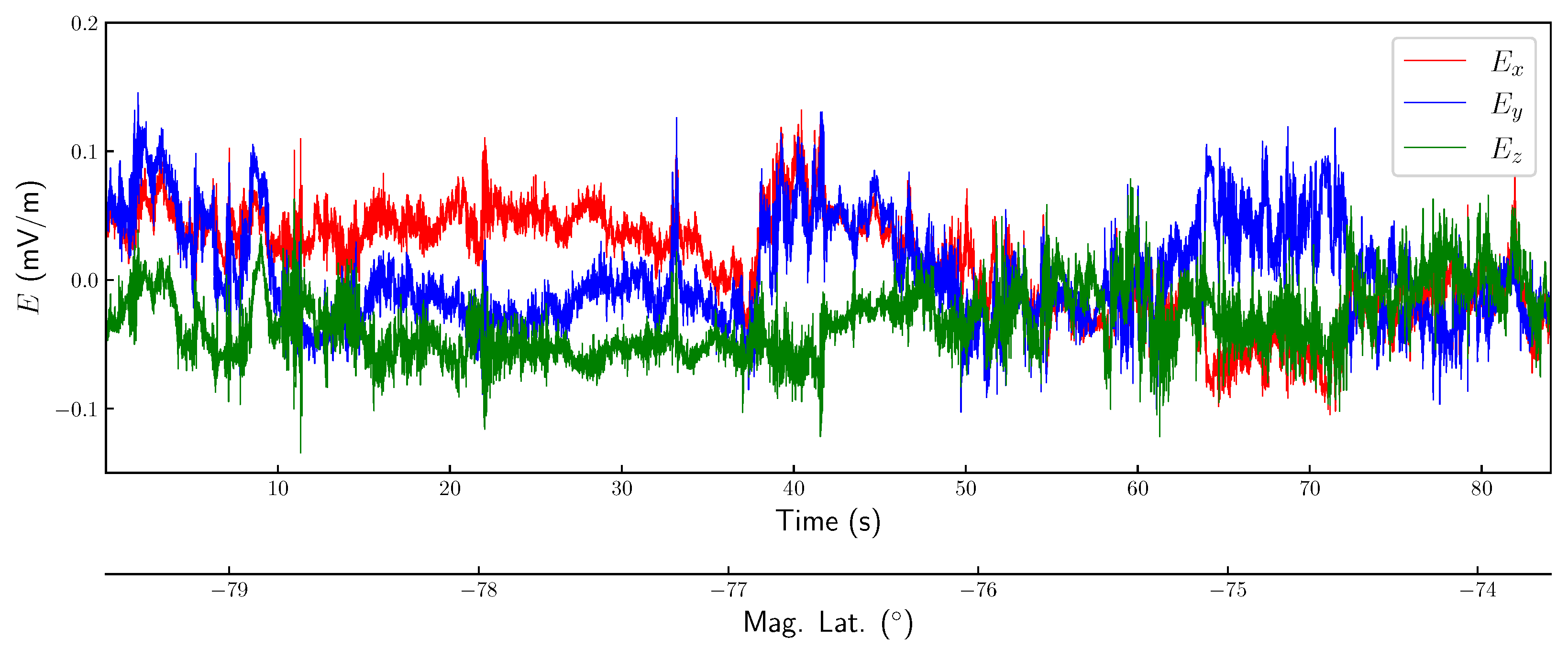
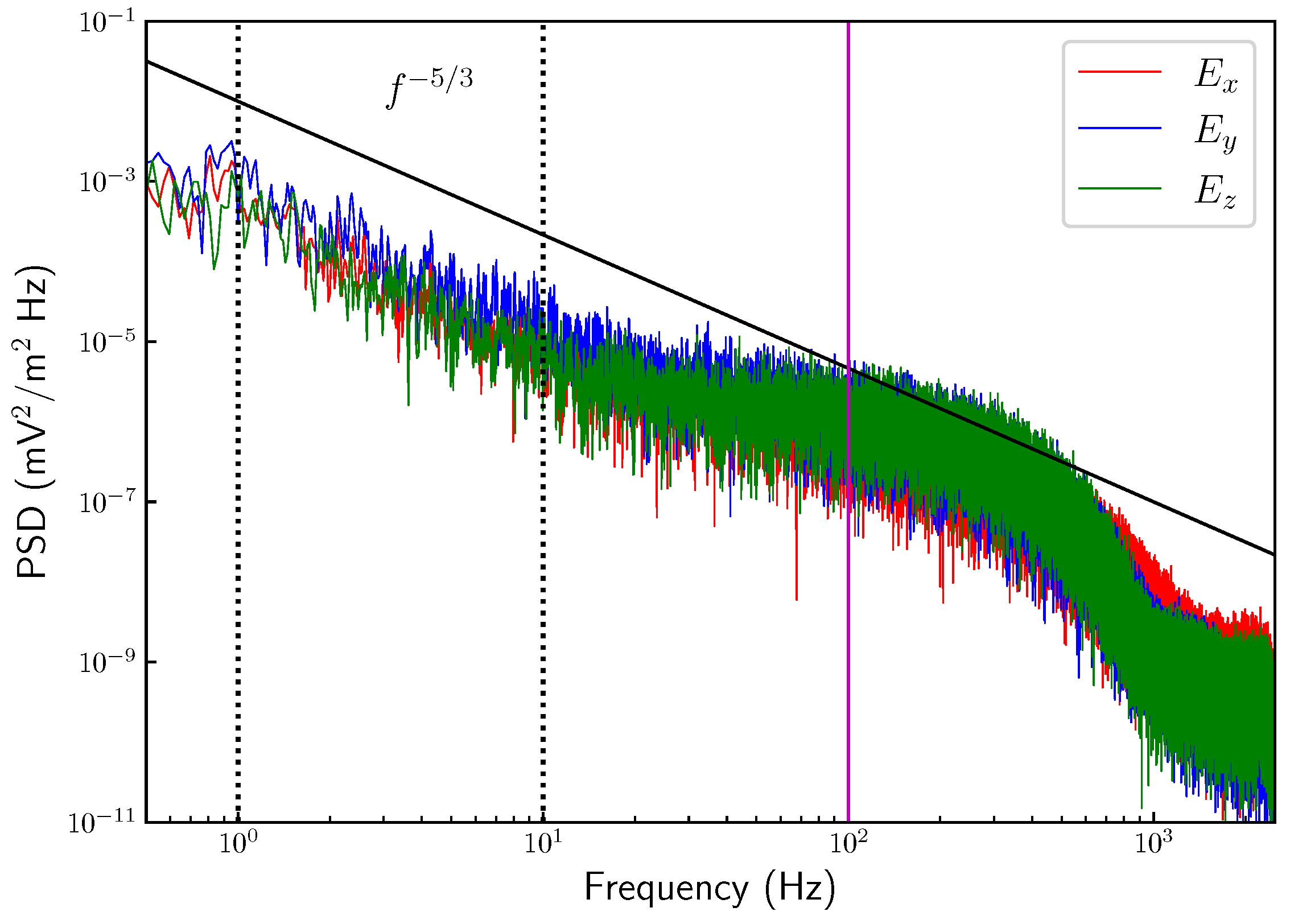
2. Data
3. Analysis and Results
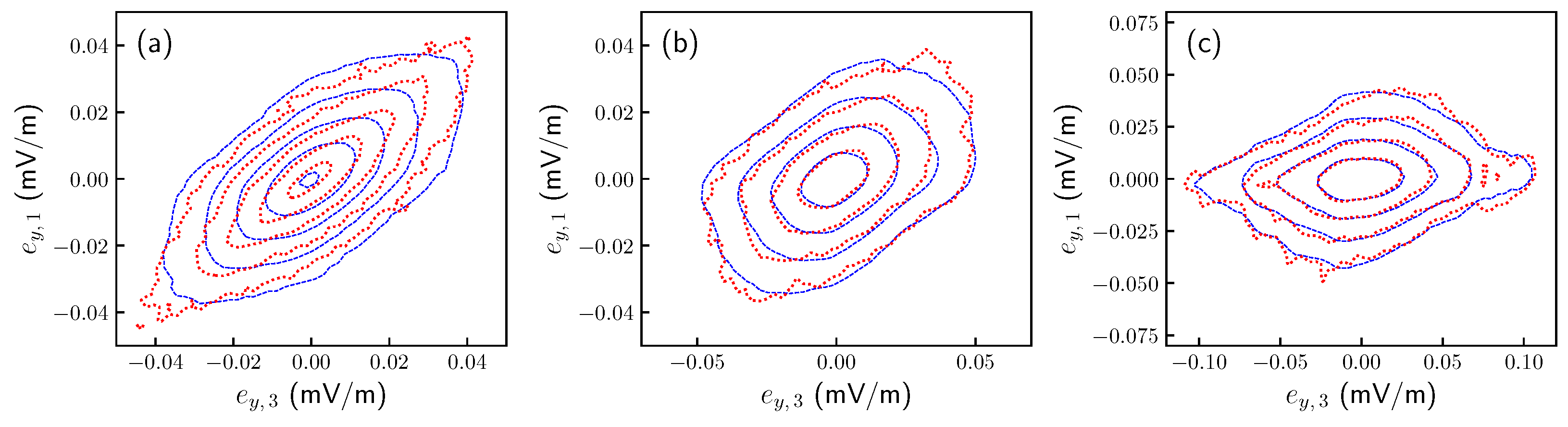
3.1. Testing the Markov Property
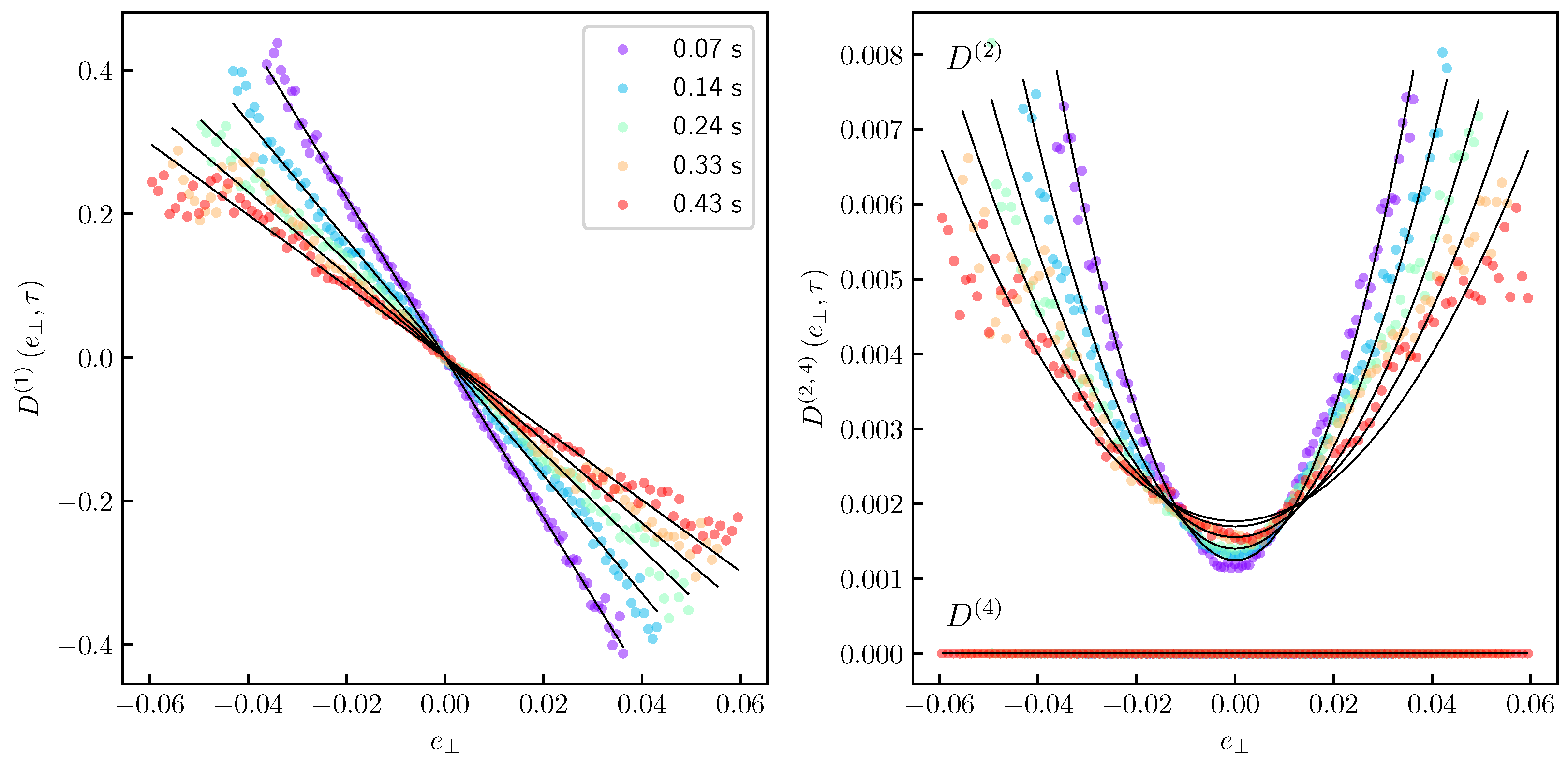
3.2. Kramers–Moyal Coefficient Analysis
3.3. Fokker–Planck Model of Electric Field Fluctuations
4. Discussion and Conclusions
Author Contributions
Funding
Data Availability Statement
Acknowledgments
Conflicts of Interest
Abbreviations
| AE | Auroral Electrojet |
| CK | Chapman–Kolmogorov |
| CSES | China-Seismo-Electromagnetic Satellite |
| EFD | Electric Field Detector |
| ELF | Extra Low Frequency |
| FPE | Fokker–Planck Equation |
| GNNS | Global Navigation Satellite System |
| GPS | Global Positioning System |
| KM | Kramers Moyal |
| MHD | Magnetohydrodynamics |
| Probability Distribution Function | |
| PSD | Power Spectral Density |
| ULF | Ultra Low Frequency |
References
- Earle, G.D.; Kelley, M.C.; Ganguli, G. Large velocity shears and associated electrostatic waves and turbulence in the auroral F region. J. Geophys. Res. Space Phys. 1989, 94, 15321–15333. [Google Scholar] [CrossRef]
- Lagoutte, D.; Cerisier, J.C.; Plagnaud, J.L.; Villain, J.P.; Forget, B. High-latitude ionospheric electrostatic turbulence studied by means of the wavelet transform. J. Atmos. Terr. Phys. 1992, 54, 1283–1293. [Google Scholar] [CrossRef]
- Kintner, P.M.; Franz, J.; Schuck, P.; Klatt, E. Interferometric coherency determination of wavelength or what are broadband ELF waves? J. Geophys. Res. 2000, 105, 21237–21250. [Google Scholar] [CrossRef]
- Hysell, D.; Shume, E. Electrostatic plasma turbulence in the topside equatorial F region ionosphere. J. Geophys. Res. Space Phys. 2002, 107, SIA-1–SIA-12. [Google Scholar] [CrossRef]
- Kintner, P.M.; Seyler, C.E. The status of observations and theory of high latitude ionospheric and magnetospheric plasma turbulence. Space Sci. Rev. 1985, 41, 1572–9672. [Google Scholar] [CrossRef]
- Golovchanskaya, I.V.; Ostapenko, A.A.; Kozelov, B.V. Relationship between the high-latitude electric and magnetic turbulence and the Birkeland field-aligned currents. J. Geophys. Res. (Space Phys.) 2006, 111, A12301. [Google Scholar] [CrossRef]
- Booker, H.G. Turbulence in the Ionosphere with Applications to Meteor-Trails Radio-Star Scintillation, Auroral Radar Echoes, and Other Phenomena. J. Geophys. Res. 1956, 61, 673–705. [Google Scholar] [CrossRef]
- Booker, H.G. A theory of scattering by nonisotropic irregularities with application to radar reflections from the aurora. J. Atmos. Terr. Phys. 1956, 8, 204–221. [Google Scholar] [CrossRef]
- Dagg, M. The origin of the ionospheric irregularities responsible for radio-star scintillations and spread-F—I. Review of existing theories. J. Atmos. Terr. Phys. 1957, 11, 133–138. [Google Scholar] [CrossRef]
- Dagg, M. The origin of the ionospheric irregularities responsible for radio-star scintillations and spread-F—II. Turbulent motion in the dynamo region. J. Atmos. Terr. Phys. 1957, 11, 139–150. [Google Scholar] [CrossRef]
- Spicher, A.; Miloch, W.J.; Clausen, L.B.N.; Moen, J.I. Plasma turbulence and coherent structures in the polar cap observed by the ICI-2 sounding rocket. J. Geophys. Res. Space Phys. 2015, 120, 10,959–10,978. [Google Scholar] [CrossRef]
- Tam, S.W.Y.; Chang, T.; Kintner, P.M.; Klatt, E. Intermittency analyses on the SIERRA measurements of the electric field fluctuations in the auroral zone. Geophys. Res. Lett. 2005, 32, L05109. [Google Scholar] [CrossRef]
- De Michelis, P.; Consolini, G.; Tozzi, R. Magnetic field fluctuation features at Swarm’s altitude: A fractal approach. Geophys. Res. Lett. 2015, 42, 3100–3105. [Google Scholar] [CrossRef]
- De Michelis, P.; Consolini, G.; Tozzi, R.; Marcucci, M.F. Scaling Features of High-Latitude Geomagnetic Field Fluctuations at Swarm Altitude: Impact of IMF Orientation. J. Geophys. Res. (Space Phys.) 2017, 122, 10,548–10,562. [Google Scholar] [CrossRef]
- Consolini, G.; De Michelis, P.; Alberti, T.; Giannattasio, F.; Coco, I.; Tozzi, R.; Chang, T.T.S. On the Multifractal Features of Low-Frequency Magnetic Field Fluctuations in the Field-Aligned Current Ionospheric Polar Regions: Swarm Observations. J. Geophys. Res. (Space Phys.) 2020, 125, e27429. [Google Scholar] [CrossRef]
- Consolini, G.; De Michelis, P.; Alberti, T.; Coco, I.; Giannattasio, F.; Tozzi, R.; Carbone, V. Intermittency and Passive Scalar Nature of Electron Density Fluctuations in the High-Latitude Ionosphere at Swarm Altitude. Geophys. Res. Lett. 2020, 47, e89628. [Google Scholar] [CrossRef]
- Consolini, G.; Quattrociocchi, V.; D’Angelo, G.; Alberti, T.; Piersanti, M.; Marcucci, M.F.; De Michelis, P. Electric Field Multifractal Features in the High-Latitude Ionosphere: CSES-01 Observations. Atmosphere 2021, 12, 646. [Google Scholar] [CrossRef]
- Consolini, G.; Quattrociocchi, V.; Benella, S.; De Michelis, P.; Alberti, T.; Piersanti, M.; Marcucci, M.F. On Turbulent Features of E × B Plasma Motion in the Auroral Topside Ionosphere: Some Results from CSES-01 Satellite. Remote Sens. 2022, 14, 1936. [Google Scholar] [CrossRef]
- Chang, T. Colloid-like Behavior and Topological Phase Transitions in Space Plasmas: Intermittent Low Frequency Turbulence in the Auroral Zone. Phys. Scr. Vol. T 2001, 89, 80–83. [Google Scholar] [CrossRef]
- Chang, T.; Tam, S.W.Y.; Wu, C.C. Complexity induced anisotropic bimodal intermittent turbulence in space plasmas. Phys. Plasmas 2004, 11, 1287–1299. [Google Scholar] [CrossRef]
- Abel, G.A.; Freeman, M.P.; Chisham, G. Spatial structure of ionospheric convection velocities in regions of open and closed magnetic field topology. Geophys. Res. Lett. 2006, 33, L24103. [Google Scholar] [CrossRef]
- Kozelov, B.V.; Golovchanskaya, I.V. Scaling of electric field fluctuations associated with the aurora during northward IMF. Geophys. Res. Lett. 2006, 33, L20109. [Google Scholar] [CrossRef]
- Abel, G.A.; Freeman, M.P.; Chisham, G.; Watkins, N.W. Investigating turbulent structure of ionospheric plasma velocity using the Halley SuperDARN radar. Nonlinear Process. Geophys. 2007, 14, 799–809. [Google Scholar] [CrossRef]
- Kozelov, B.V.; Golovchanskaya, I.V.; Ostapenko, A.A.; Fedorenko, Y.V. Wavelet analysis of high-latitude electric and magnetic fluctuations observed by the Dynamic Explorer 2 satellite. J. Geophys. Res. (Space Phys.) 2008, 113, A03308. [Google Scholar] [CrossRef]
- Kozelov, B.V.; Golovchanskaya, I.V. Derivation of aurora scaling parameters from ground-based imaging observations: Numerical tests. J. Geophys. Res. (Space Phys.) 2010, 115, A02204. [Google Scholar] [CrossRef]
- Golovchanskaya, I.V.; Kozelov, B.V. On the origin of electric turbulence in the polar cap ionosphere. J. Geophys. Res. (Space Phys.) 2010, 115, A09321. [Google Scholar] [CrossRef]
- Golovchanskaya, I.V.; Kozelov, B.V. Properties of electric turbulence in the polar cap ionosphere. Geomagn. Aeron. 2010, 50, 576–587. [Google Scholar] [CrossRef]
- Tam, S.W.Y.; Chang, T.; Kintner, P.M.; Klatt, E.M. Rank-ordered multifractal analysis for intermittent fluctuations with global crossover behavior. Phys. Rev. E 2010, 81, 036414. [Google Scholar] [CrossRef]
- Tam, S.W.Y.; Chang, T. Double rank-ordering technique of ROMA (Rank-Ordered Multifractal Analysis) for multifractal fluctuations featuring multiple regimes of scales. Nonlinear Process. Geophys. 2011, 18, 405–414. [Google Scholar] [CrossRef]
- Frisch, U. Turbulence; Cambridge University Press: Cambridge, UK, 1995. [Google Scholar]
- Pedrizzetti, G.; Novikov, E.A. On Markov modelling of turbulence. J. Fluid Mech. 1994, 280, 69–93. [Google Scholar] [CrossRef]
- Friedrich, R.; Peinke, J. Description of a turbulent cascade by a Fokker-Planck equation. Phys. Rev. Lett. 1997, 78, 863. [Google Scholar] [CrossRef]
- Strumik, M.; Macek, W.M. Testing for Markovian character and modeling of intermittency in solar wind turbulence. Phys. Rev. E 2008, 78, 026414. [Google Scholar] [CrossRef] [PubMed]
- Strumik, M.; Macek, W. Statistical analysis of transfer of fluctuations in solar wind turbulence. Nonlinear Process. Geophys. 2008, 15, 607–613. [Google Scholar] [CrossRef][Green Version]
- Benella, S.; Stumpo, M.; Consolini, G.; Alberti, T.; Carbone, V.; Laurenza, M. Markovian Features of the Solar Wind at Subproton Scales. Astrophys. J. Lett. 2022, 928, L21. [Google Scholar] [CrossRef]
- Benella, S.; Stumpo, M.; Consolini, G.; Alberti, T.; Laurenza, M.; Yordanova, E. Kramers–Moyal analysis of interplanetary magnetic field fluctuations at sub-ion scales. Rend. Lincei. Sci. Fis. E Nat. 2022, 33, 721–728. [Google Scholar] [CrossRef]
- Renner, C.; Peinke, J.; Friedrich, R. Experimental indications for Markov properties of small-scale turbulence. J. Fluid Mech. 2001, 433, 383. [Google Scholar] [CrossRef]
- Huang, J.; Lei, J.; Li, S.; Zeren, Z.; Li, C.; Zhu, X.; Yu, W. The Electric Field Detector (EFD) onboard the ZH-1 satellite and first observational results. Earth Planet. Phys. 2018, 2, 469–478. [Google Scholar] [CrossRef]
- Papini, E.; Piersanti, M.; D’Angelo, G.; Cicone, A.; Bertello, I.; Parmentier, A.; Diego, P.; Ubertini, P.; Consolini, G.; Zhima, Z. Detecting the Auroral Oval through CSES-01 Electric Field Measurements in the Ionosphere. Remote Sens. 2023, 15, 1568. [Google Scholar] [CrossRef]
- Pécseli, H. Spectral properties of electrostatic drift wave turbulence in the laboratory and the ionosphere. In Annales Geophysicae; Copernicus GmbH: Göttingen, Germany, 2015; Volume 33, pp. 875–900. [Google Scholar]
- Mounir, H.; Berthelier, A.; Cerisier, J.C.; Lagoutte, D.; Beghin, C. The small-scale turbulent structure of the high latitude ionosphere-Arcad-Aureol-3 observations. Ann. Geophys. 1991, 9, 725–737. [Google Scholar]
- Basu, S.; MacKenzie, E.; Basu, S.; Coley, W.R.; Sharber, J.R.; Hoegy, W.R. Plasma structuring by the gradient drift instability at high latitudes and comparison with velocity shear driven processes. J. Geophys. Res. 1990, 95, 7799–7818. [Google Scholar] [CrossRef]
- Risken, H.; Caugheyz, T.K. The Fokker-Planck Equation: Methods of Solution and Application, 2nd ed. J. Appl. Mech. 1991, 58, 860. [Google Scholar] [CrossRef]
- Castaing, B.; Gagne, Y.; Hopfinger, E.J. Velocity probability density functions of high Reynolds number turbulence. Phys. D Nonlinear Phenom. 1990, 46, 177–200. [Google Scholar] [CrossRef]
- Sorriso-Valvo, L.; Carbone, V.; Veltri, P.; Consolini, G.; Bruno, R. Intermittency in the solar wind turbulence through probability distribution functions of fluctuations. Geophys. Res. Lett. 1999, 26, 1801–1804. [Google Scholar] [CrossRef]
- Sorriso-Valvo, L.; Marino, R.; Lijoi, L.; Perri, S.; Carbone, V. Self-consistent Castaing Distribution of Solar Wind Turbulent Fluctuations. Astrophys. J. 2015, 807, 86. [Google Scholar] [CrossRef]
- Nickelsen, D.; Engel, A. Probing small-scale intermittency with a fluctuation theorem. Phys. Rev. Lett. 2013, 110, 214501. [Google Scholar] [CrossRef]
- Fuchs, A.; Obligado, M.; Bourgoin, M.; Gibert, M.; Mininni, P.D.; Peinke, J. Markov property of Lagrangian turbulence. EPL (Europhys. Lett.) 2022, 137, 53001. [Google Scholar] [CrossRef]
- Marcq, P.; Naert, A. A Langevin equation for the energy cascade in fully developed turbulence. Phys. D Nonlinear Phenom. 1998, 124, 368–381. [Google Scholar] [CrossRef]
- Marcq, P.; Naert, A. A Langevin equation for turbulent velocity increments. Phys. Fluids 2001, 13, 2590–2595. [Google Scholar] [CrossRef]
- Chang, T.; Tam, S.W.; Wu, C.C. Complexity in space plasmas—A brief review. Space Sci. Rev. 2006, 122, 281–291. [Google Scholar] [CrossRef]
- Yordanova, E.; Bergman, J.; Consolini, G.; Kretzschmar, M.; Materassi, M.; Popielawska, B.; Roca-Sogorb, M.; Stasiewicz, K.; Wernik, A. Anisotropic scaling features and complexity in magnetospheric-cusp: A case study. Nonlinear Process. Geophys. 2005, 12, 817–825. [Google Scholar] [CrossRef]
- Gondarenko, N.; Guzdar, P. Density and electric field fluctuations associated with the gradient drift instability in the high-latitude ionosphere. Geophys. Res. Lett. 2004, 31, L11802. [Google Scholar] [CrossRef]
- Gondarenko, N.; Guzdar, P. Plasma patch structuring by the nonlinear evolution of the gradient drift instability in the high-latitude ionosphere. J. Geophys. Res. Space Phys. 2004, 109, A09301. [Google Scholar] [CrossRef]


| A | |||
Disclaimer/Publisher’s Note: The statements, opinions and data contained in all publications are solely those of the individual author(s) and contributor(s) and not of MDPI and/or the editor(s). MDPI and/or the editor(s) disclaim responsibility for any injury to people or property resulting from any ideas, methods, instructions or products referred to in the content. |
© 2023 by the authors. Licensee MDPI, Basel, Switzerland. This article is an open access article distributed under the terms and conditions of the Creative Commons Attribution (CC BY) license (https://creativecommons.org/licenses/by/4.0/).
Share and Cite
Benella, S.; Quattrociocchi, V.; Papini, E.; Stumpo, M.; Alberti, T.; Marcucci, M.F.; De Michelis, P.; Piersanti, M.; Consolini, G. Modeling Turbulent Fluctuations in High-Latitude Ionospheric Plasma Using Electric Field CSES-01 Observations. Atmosphere 2023, 14, 1466. https://doi.org/10.3390/atmos14091466
Benella S, Quattrociocchi V, Papini E, Stumpo M, Alberti T, Marcucci MF, De Michelis P, Piersanti M, Consolini G. Modeling Turbulent Fluctuations in High-Latitude Ionospheric Plasma Using Electric Field CSES-01 Observations. Atmosphere. 2023; 14(9):1466. https://doi.org/10.3390/atmos14091466
Chicago/Turabian StyleBenella, Simone, Virgilio Quattrociocchi, Emanuele Papini, Mirko Stumpo, Tommaso Alberti, Maria Federica Marcucci, Paola De Michelis, Mirko Piersanti, and Giuseppe Consolini. 2023. "Modeling Turbulent Fluctuations in High-Latitude Ionospheric Plasma Using Electric Field CSES-01 Observations" Atmosphere 14, no. 9: 1466. https://doi.org/10.3390/atmos14091466
APA StyleBenella, S., Quattrociocchi, V., Papini, E., Stumpo, M., Alberti, T., Marcucci, M. F., De Michelis, P., Piersanti, M., & Consolini, G. (2023). Modeling Turbulent Fluctuations in High-Latitude Ionospheric Plasma Using Electric Field CSES-01 Observations. Atmosphere, 14(9), 1466. https://doi.org/10.3390/atmos14091466