Abstract
Air pollutants adversely affect human health, and thus a global improvement in air quality is urgent. A Geostationary Environment Monitoring Spectrometer (GEMS) was mounted on the geostationary Chollian 2B satellite in 2020 to observe the spatial distribution of air pollution, and sequential observations have been released since July 2022. The reliability of GEMS must be analyzed because it is the first payload on the geostationary Earth orbit satellite to observe trace gases. This study analyzed the initial results of GEMS observations such as the aerosol optical depth and vertical column densities (VCD) of ozone (O3), nitrogen dioxide (NO2), sulfur dioxide (SO2), and formaldehyde (HCHO), and compared them with previous studies. The correlation coefficient of O3 ranged from 0.90 (Ozone Monitoring Instrument, OMI) to 0.97 (TROPOspheric Monitoring Instrument, TROPOMI), whereas that of NO2 ranged from 0.47 (winter, OMI and OMPS) to 0.83 (summer, TROPOMI). GEMS yielded a higher VCD of NO2 than that of OMI and TROPOMI. Based on the sources of O3 and NO2, GEMS observed the maximum VCD at a different time (3–4 h) to that of the ground observations. Overall, GEMS can make observations several times a day and is a potential tool for atmospheric environmental analysis.
1. Introduction
Outdoor air pollution adversely affects health and can cause carcinogenicity [1,2,3,4,5]. According to the World Health Organization, air pollutants caused approximately seven million premature deaths worldwide in 2012, with low- and middle-income countries accounting for 91% [6]. Particularly, due to the deteriorating air quality due to rapid economic growth, the East Asian region has recently reported high levels of air pollutants and is therefore striving to improve the air quality. The effects of both the long-range transported and locally emitted air pollutants need to be considered for an effective improvement in air quality. Studies have attempted to elucidate that the mutual effects between air quality and air pollutants are not linear due to secondary aerosols, among other factors [7,8,9,10,11,12,13].
Most studies have used numerical modeling to analyze these mutual effects, and various complementary methods to resolve the uncertainty yielded by the model results have been reviewed and introduced [14,15,16]. As the concentration of trace gases in the atmosphere can be observed using remote sensing technology, several low Earth orbit (LEO) satellites have been used [17,18,19,20,21]. Recently, it has become feasible to observe from geostationary orbit satellites [22]. The Geostationary Environment Monitoring Spectrometer (GEMS) was mounted on Chollian 2B (GeoKOMPSAT-2B), a geostationary Earth orbit (GEO) satellite launched in 2020. GEMS can observe the atmospheric environment of East Asia 6–10 times a day, thereby reducing the space–time limitation of the satellite [23,24]. The verification of various methods for reliability analysis is essential because GEMS is the first air quality species observation payload operated in GEO.
In this study, to ensure the reliability of GEMS observations, the spatial distribution of the East Asian region was analyzed using the initial data of the pilot operation and compared with that reported in previous studies [25,26,27,28,29,30,31,32,33,34,35,36,37,38,39,40,41,42]. The reliability was analyzed by comparing it with the data observed from an existing LEO satellite.
2. Materials and Methods
2.1. GEMS
GEMS was mounted on a geostationary satellite, the Chollian 2B satellite (GeoKOMPSAT-2B; GK2B), to target a spatial region (in the 5° S–45° N, 75° E–145° E directions). Spatial resolution ranges from 4.8 to 25.6 km, depending on the latitude; the farther away from the equator, the lower the spatial resolution [24]. Specifically, GEMS has a ground sampling distance at a resolution of 8 km E–W and 7 km N–S with respect to Seoul, Korea. GEMS observes a spectral region of 300–500 nm input data for Level 2 [23] at 0.2 nm with a sampling ratio of 3 (resolution full-width half maximum of 0.6 nm). It has more than 20 products including the vertical column densities (VCDs) of ozone (O3), nitrogen dioxide (NO2), sulfur dioxide (SO2), and formaldehyde (HCHO) as well as the aerosol optical depth (AOD). The Geostationary Ocean Color Imager-II (GOCI-2) [43] was also mounted on the same satellite; GEMS/GOCI-2 alternately records hourly observations, with 30-minute intervals between every 30 min of observation. The specifications of GEMS are listed in Table 1.

Table 1.
Specifications of the Geostationary Environment Monitoring Spectrometer (GEMS).
GEMS creates a data cube containing three-dimensional data for a single observation. One axis is in the E–W direction, another in the N–S direction, and the last is in the spectral range. GEMS moves the scan mirror 695 times within 30 min from west to east, each time comprising two-dimensional data using one slit. Each slit has spatial information composed of 2048 pixels in the N–S direction, whereas the other direction is divided into 1000 pieces of spectral information. As the solar zenith angle (SZA) changes over time, the number of scan mirror movements in the E–W direction of the GEMS observation domain changes, whereas the number of observations per day varies (Figure 1). When the signal is low due to the low solar altitude such as during winter, GEMS records relatively fewer observations over a relatively small area; when the daytime becomes longer such as in summer, it records more observations. GEMS calculates the change in the SZA every 15 d in the domain, predicts change in the signal-to-noise ratio (SNR) according to the SZA, and establishes the observation schedule (Table 2). Accordingly, GEMS reordered the observations six times in January and 10 times from April to September, per day. Spatially, the scan areas from west to east were divided into either full-disk observations (full central [FC], full west [FW]), which entailed observing 695 slits for 30 min, or half-disk observations (half east [HE], half Korea [HK]), where one slit was observed twice to increase the SNR.
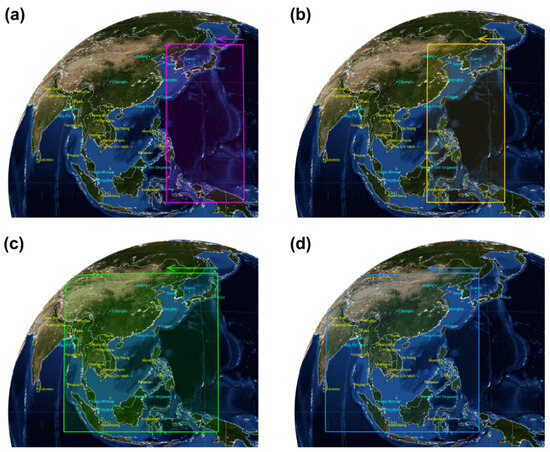
Figure 1.
Classification of observation areas of the Geostationary Environment Monitoring Spectrometer (GEMS). The purple box in (a) indicates half east (HE), the yellow box in (b) indicates half Korea (HK), the green box in (c) indicates full central (FC), and the blue box in (d) indicates full west (FW). The arrows indicate the scanning direction.
Table 2.
Observation schedule according to each month.
2.2. Datasets
Regarding the observation results of GEMS, Levels 0, 1a, 1b, 2, and 3 were generated, similar to the general satellite data, and 1c and value-added product (VAP) data were also produced. Level 0 represents the original observed spectral data, 1a the wavelength correction, 1b the geographic correction, and 1c the spectral correction performed on 1b data. Level 2 represents various outputs such as the concentration of trace gases in the atmosphere and the ultraviolet (UV) index. Level 3 represents the average length, and VAP represents general Level 4. In this study, the pilot calculation results for Levels 1c and 2 observed by GEMS were disclosed, and their characteristics were analyzed.
Total column observations of O3 and NO2 observed by GEMS during the pilot operation were compared with the observations by the Ozone Monitoring Instrument (OMI) [18] onboard Aura and the TROPOspheric Monitoring Instrument (TROPOMI) [20] onboard Sentinel-5P. O3 measurements were also compared with the ones from the Ozone Mapping and Profiler Suite (OMPS) [21] onboard the Suomi National Polar-orbiting Partnership. OMI Level 3 data, which are gridded, were used; however, Level 2 data for the other satellites were used because the Level 3 data were not available. The test operation period of GEMS was from November 2020 to June 2022, and data from 1 March 2021 to 28 February 2022 were considered for the analysis. The GEMS observation domain described in Section 2.1 was the study area. The data from each LEO satellite excluded data outside the GEMS observation area. To analyze the diurnal changes in the GEMS observation results, the average ground observation data in Seoul were used for comparison. The satellite data were removed when the viewing zenith angle was over 60°.
To validate the observed O3 VCD from GEMS, the total column O3 data observed by the Dobson O3 spectrophotometer located at Yonsei University in Seoul, Korea, were used. The vertical O3 concentration data observed by the Dobson O3 spectrophotometer were used, and the hourly mean concentration was determined by selecting the representative value of the concentration observed from 30 min before to the corresponding hour, considering that GEMS observes for 30 min every hour starting at 45 min past the hour. Values observed below 200 DU or above 500 DU were considered outliers and excluded from the analysis. Additionally, times with fewer than five observations were excluded from the analysis.
2.3. Methods
2.3.1. GEMS Algorithm
The GEMS system utilizes algorithms to retrieve parameters such as O3, NO2, SO2, AOD, HCHO/CHOCHO, UV index, surface reflectance, and cloud detection. In this section, the O3, NO2, SO2, AOD, and HCHO algorithms are briefly discussed. For more comprehensive information, additional details can be found in the algorithm technical basis documents available on the website of the National Institute of Environmental Research (NIER), which operates GEMS [http://nesc.nier.go.kr (accessed on 18 September 2023)].
GEMS observes solar irradiance daily at an angle of incidence of 29° [23]. The nonlinear least squares method is used to correct the spectral response function (SRF) of the daily observed solar irradiance with solar irradiance data observed at 0.01 nm intervals at the Smithsonian Astrophysical Observatory in the United States [44]. After SRF correction, polarization correction is applied to Level 1c data [45] calculated using optimal convolution variables based on a stable observation schedule following the launch of GEMS. Next, surface reflectance is computed, and based on this information, the calculations for clouds and aerosols are performed. Subsequently, O3 is calculated, followed by the computation of other substances such as SO2, NO2, HCHO/CHOCHO, and the UV index.
The GEMS O3 profile algorithm uses the optimal estimation method, a well-established technique employed by OMI and LEO satellites and adopted as a GEMS operational algorithm. The GEMS total ozone algorithm is based on the NASA TOMS, version 9, algorithm [46] and is composed of a forward model and an inverse model. The forward model calculates radiance and Jacobians at various wavelengths (312.5, 317.34, 331.02, 340, 380 nm) at the top of the atmosphere using VLIDORT [47]. The inverse model is employed to convert measured radiance into geophysical parameters for remote sensing and comprises a three-step process. In Step 1, measurements at 340 and 380 nm are used to calculate reflectivity. Then, from the radiance calculated by the VLIDORT, the observed radiance at 317.34 nm is determined, and subsequently, the total column of O3 (TCO) is estimated. Finally, a temperature correction is applied. In Step 2, using the variables derived in Step 1, optimal estimation [48] is applied to calculate ozone profiles at three wavelengths (312.34, 317.34, 331.02 nm), and TCO is obtained by summing the ozone profiles. In Step 3, cloud corrections are performed, but these corrections are applied under certain conditions. Cloud corrections are not performed if there are no clouds, if snow/ice is present, or if the is lower than . For other cases where , a linear correction factor () is calculated as , where . Here, represents the Lambertian equivalent reflectance (LER) at 340 nm, and and are assumed to be 0.05 and 0.4, respectively. In cases where there is no snow/ice and , is estimated from LER at 340 nm, assuming and , then the following correction is applied.
In these equations, represents the O3 value of layer computed in Step 2, is the O3 value of layer from the a priori profile used in Step 2, and represents the layer efficiency. The corrected the total O3 value is then expressed as:
The NO2 algorithm calculates the slant column density (SCD) using a wavelength ranging from 432 to 450 nm as a fitting window via differential optical absorption spectroscopy (DOAS) and air mass factor (AMF) to calculate the vertical integral concentration; afterward, the VCD can be obtained.
The SO2 algorithm uses the principal component analysis method that calculates the concentration based on the observation data at the point where SO2 is expected not to exist, and the DOAS algorithm uses the 325–335 nm-wavelength range as a fitting window.
The spectral observation region of GEMS ranges from 300 to 500 nm. Therefore, the 550-nm wavelength region, which generally produces AOD, cannot be observed. GEMS calculates AOD using the lookup table determined in advance using spectral information for six wavelengths (354, 388, 412, 443, 477, and 490 nm). One of three options is used: 30-day composite GEMS surface reflectance using the minimum reflectance method obtained from the GEMS AERAOD algorithm, or GEMS climatology surface reflectance using the minimum reflectance method. The OMI climatology LER (OMLER v003) dataset is utilized only when GEMS data are unavailable for surface reflectance correction [37].
The GEMS HCHO algorithm utilizes the wavelength range of 328.5–356.5 nm and employs the BOAS method. It estimates clean regions and uses the measured radiance values from those regions as reference data. After applying the HCHO algorithm of GEMS using the Level 1b data of OMI, the correlation coefficient for SCD was calculated to be 0.74 [49].
2.3.2. Data Processing
As GEMS records more observations in summer and fewer in winter, seasonal characteristics can be reflected in the spatial distribution. Therefore, only the data observed between 12:45 and 13:15, near the observation time of the LEO satellites, were used. However, to analyze the temporal changes in VCD for O3 and NO2, the data observed in the Seoul area at all times were used.
For a comparison with the data obtained by the LEO satellites, the Level 2 data of GEMS, TROPOMI, and OMPS were gridded at 0.25° × 0.25° (OMI Level 3 grid). The median value (i.e., the number at the center when the observations of the entire group are arranged in order of size corresponding to each grid) was used for gridding.
3. Results
3.1. Level 1c Product Assessment
Regarding the corresponding observation results, data in the spring and autumn equinoxes were similar regardless of the north–south direction (Figure 2). However, the solar irradiance values were lower in the northern region (Seoul) of the focal plane than in the opposite side (equator), with opposite trends during the winter solstice.
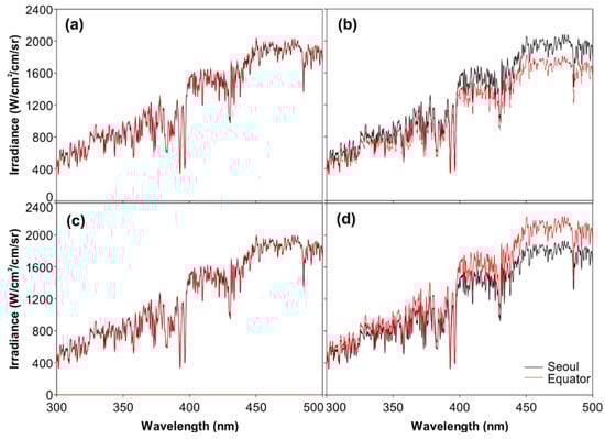
Figure 2.
Solar irradiance observed using GEMS. For Seoul (black lines) and the equator (red lines) at (a) vernal equinox, (b) summer solstice, (c) autumn equinox, and (d) winter solstice.
Figure 3 shows the spatial distribution showing the difference between the short (350 nm) and long (455 nm) wavelength of GEMS Level 1c observed at the solstice (12:45–13:15) in the spring/autumn/summer/winter equinox. Wavelengths that seemed to have the least absorption of trace gases were selected according to the results of the atmospheric radiation transfer model [45]. Because the long-wavelength radiation of Level 1c is twice the short-wavelength radiation, a simple comparison is difficult. Accordingly, the maximum value of the radiation amount of the two wavelengths was normalized to 1, and the normalized value of the short wavelength was compared with that of the long wavelength. Generally, pixels with numerous clouds appeared blue with a large radiance at a short wavelength as the amount of reflected radiation from the upper part of the atmosphere. Conversely, as the amount of radiation reflected from the ground was observed in pixels without clouds, the amount of absorption and scattering by the atmosphere of the short wavelength exceeded that of the long wavelength; thus, the long wavelength was expressed as a strong red.
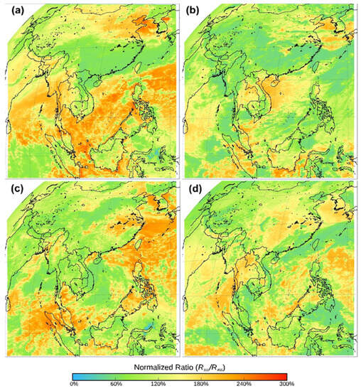
Figure 3.
Level 1c ratios of the 350 nm and 455 nm normalized radiance observed in (a) vernal equinox, (b) summer solstice, (c) autumn equinox, and (d) winter solstice at 03:45–04:15 (UTC) in 2021. The region in blue indicates that the change width of the short wavelength (350 nm) was larger than that of the long wavelength (455 nm) in the red region.
3.2. Level 2 Product Analysis
3.2.1. Spatiotemporal Distribution of Ozone
Figure 4 displays the seasonal mean spatial distribution of the TCO and O3 between the cloud optical centroid pressure and the surface, observed using FW in clear skies. The spatial distribution of the TCO remains relatively consistent due to the prevalence of O3 in the stratosphere, with higher concentrations at high latitudes during spring and winter seasons [25]. However, O3 between the cloud optical centroid pressure and the surface exhibits distinct spatial and temporal variations. Particularly, the eastern region of India shows relatively high values during spring and relatively low values during summer, autumn, and winter [26]. In the region of Northeast Asia, O3 levels increase from spring, reach their peak in summer, decrease in autumn, and reach their lowest values in winter. These O3 variations are attributed to anthropogenic pollutant emissions in the Northeast Asian region and intensified ultraviolet radiation during summer [27,28]. Additionally, in the Indochina Peninsula, ozone concentrations are higher in spring than in summer. This is attributed to the fact that during spring, the region reports increased emissions of ozone precursors due to biomass burning activities such as wildfires, creating conditions favorable for ozone production. In contrast, reduced biomass burning activities and the monsoon season during summer lead to decreased emissions of ozone precursors, resulting in less favorable conditions for ozone production than those during spring [29,30]. GEMS’ ability to observe variations in O3 concentrations caused by anthropogenic pollutants emitted at the ground level makes it a valuable tool for analyzing anthropogenic O3 production and depletion in these regions.
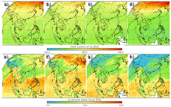
Figure 4.
Spatial distribution of the average seasonal total column O3 and O3 between the cloud optical centroid pressure and the surface is shown. The panels depict O3 concentrations for (a,e) spring (1 March 2021–31 May 2021), (b,f) summer (1 June 2021–31 August 2021), (c,g) autumn (1 September 2021–30 November 2021), and (d,h) winter (1 December 2021–28 February 2022). Panels (a–d) represent the total column O3, while panels (e–h) represent O3 between the cloud optical centroid pressure and the surface.
To compare the data obtained using the GEMS and LEO satellites (OMI and TROPOMI), the absolute values and correlation coefficients between GEMS and OMI, and GEMS and TROPOMI were calculated (Figure 5). The correlation coefficient (r) of the VCD of the O3 concentrations obtained using OMI and GEMS was 0.90, and that obtained using TROPOMI and GEMS was 0.97. These results imply that the values obtained by the three satellites were similar.
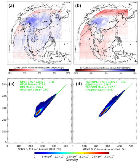
Figure 5.
Spatial distribution using the median O3 concentrations observed via GEMS, Ozone Monitoring Instrument (OMI), and TROPOspheric Monitoring Instrument (TROPOMI) for one year (1 March 2021 to 28 February 2022): (a) (GEMS-OMI)/GEMS and (b) (GEMS-TROPOMI)/GEMS. The distributions between the two results: (c) GEMS vs. OMI and (d) GEMS vs. TROPOMI.
In the spatial distribution of the O3 VCD using GEMS and OMI, the values of GEMS were generally higher than those of OMI. However, the values of OMI were higher in western India, south of the equator, northern China, and Mongolia compared with those of GEMS in these regions. Both the averaged absolute values of OMI and GEMS were 277 DU and 278 DU and those of TROPOMI and GEMS were 278 DU and 277 DU, respectively, which were similar. The reason for the difference in these GEMS O3 values was that the observing points of OMI and TROPOMI were not the same; thus, the subpopulations in GEMS were different. GEMS recorded higher O3 VCD values than TROPOMI in Laos, Bhutan, southern China, and near the equator over which GEMS was located at 128.2°E. In northern China, Myanmar, Malaysia, Bangladesh, India, Indonesia, and the oceans, TROPOMI had higher values.
Due to the diurnal variation in O3 VCD, a comparison analysis was performed between the Dobson data, which presents the total O3 concentration from the ground, and the GEMS time-observation results for the analysis are presented in Figure 6a. The Dobson data are not regularly observed periodically; the data are observed once a day or intermittently several times. Thus, the observation frequency is itself less than that of GEMS and is also irregular. The vertical O3 concentration data observed by the Dobson zenith-sky observations for 1 year were collected, and the results were compared by excluding the hours in which the data were observed for less than five times in total. The GEMS and Dobson observation results showed a high correlation (r = 0.94) over the day; however, the GEMS observation results produced lower values compared with those produced by Dobson (Dobson = GEMS × 1.01 + 6.73). Additionally, GEMS and Dobson showed maximum values at 12:45–13:15 and 12:30–13:30, respectively, whereas the concentration change over time in GEMS was not significant at 8 DU, which was only 2.49% of the maximum value; Dobson showed a difference of about 18 DU per day, which was approximately 5.25% of the maximum concentration.
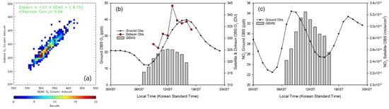
Figure 6.
Comparison of vertical column density (VCD, molecular number /cm3) of O3 between GEMS and Dobson from Yonsei University in Seoul from 1 March 2021, to 28 February 2022 (a), the temporal variations of VCD of O3 from GEMS and Dobson, and ground station O3 concentration (ppb) (b). Same as (b), but for NO2 from GEMS and the ground station (c).
The ground O3 concentration was lowest at 08:00 and reached its peak at 16:00. However, the GEMS-observed O3 VCD showed its highest values at 12:45–13:15, peaking 3 h earlier than the ground O3 concentration. For NO2, anthropogenic pollutants generated at the ground level undergo transport and accumulation in the troposphere. In contrast, O3 is predominantly influenced by stratospheric O3, where temporal changes in O3 are primarily driven by photochemical reaction mechanisms responsible for O3 production and depletion in the stratosphere.
That is, as solar radiation was strongest at noon, the photochemical reaction was also most active, which corresponded to the maximum value of O3 observed in GEMS at 12:45–13:15. Thereafter, the concentration of O3 decreased as the radiation decreased. Conversely, in the case of NO2, the contribution of NO2 emissions by means of transportation was the largest. Therefore, the ground concentration was highest at 08:00 during rush hour traffic, and it spread vertically and accumulated at the highest value at 11:45–12:15, which was a 4 h gap difference. Regarding LEO satellites, which recorded observations approximately once a day, analyzing such diurnal changes in the O3 and NO2 concentrations was difficult. In contrast, GEMS could observe the same places up to 10 times a day and observing changes based on the time of day was possible. Evidently, changes in O3 and NO2 concentrations could be determined.
3.2.2. Spatiotemporal Distribution of Nitrogen Dioxide and Sulfur Dioxide Concentrations
Figure 7 presents the spatial distribution of the seasonal average of VCD for NO2 observed by GEMS. The Northeast Asian region has, by far, the highest NO2 concentration among the GEMS domains. Seasonally, the VCD of NO2 was highest in winter, followed by autumn, spring, and summer. Seasonal changes were consistent with those reported in previous studies that used satellite observations [31,32,33]. In Northeast Asia, the NO2 concentration was highest in eastern China and the metropolitan area of Korea; these results were similar to those observed by air quality observation satellites OMI and SCIAMACHY [34,35]. In India, the NO2 concentration in urban areas including New Delhi was high, consistent with existing satellite observation results [36]. In the Indochina Peninsula, high concentration spots of NO2 were detected in Bangkok, Kuala Lumpur, and Singapore, and the concentration was high on the shipping route to the South China Sea through Malaysia.
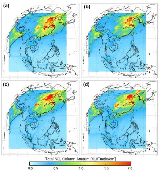
Figure 7.
Seasonal average of Level 2 NO2 total concentration observed in 2021 at 12:45–13:15 (KST): (a) spring, (b) summer, (c) autumn, and (d) winter.
Figure 8 shows the difference in VCD for NO2 observed by GEMS, OMI, TROPOMI, and OMPS in Beijing, Shanghai, and Seoul, which are major cities in Northeast Asia. The observed NO2 VCD varied between the three cities, but they appeared to exhibit a relatively correlated pattern. Furthermore, GEMS showed higher concentrations compared to other LEO satellites. The correlation coefficient between the GEMS observations and LEO satellite observations was relatively high in spring (OMI and OMPS) and summer (TROPOMI) but low in winter (Table 3). GEMS had the lowest r value with OMPS and showed high correlations with OMI and TROPOMI. The weak correlation between GEMS and the LEO satellite, in contrast to previous findings [50], (r = 0.93–0.95 between OMI and TROPOMI), was presumed to be attributed to various factors including disparities in orbit and algorithmic approaches. The precise causes will be thoroughly analyzed through further research to elucidate the underlying factors. However, the averaged VCD of NO2 by GEMS was 10% (OMPS, summer) to 38% (TROPOMI and OMPS, winter), higher than that by the LEO satellites (OMI, TROPOMI, and OMPS).
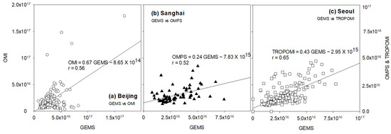
Figure 8.
Correlation diagram for the seasonal analysis of the median NO2 VCD observed by GEMS, OMI, TROPOMI, and Ozone Mapping and Profiler Suite (OMPS). (a) GEMS vs. OMI at Beijing; (b) GEMS vs. OMPS at Shanghai; (c) GEMS vs. TROPOMI at Seoul.
Table 3.
Correlation coefficient (r) between the VCDs of NO2 observed via GEMS and the LEO satellites.
A previous study reported a VCD of NO2 from OMI and TROPOMI of 30%–50% lower than that from the terrestrial Multi AXis (MAX)-DOAS observation [51], which seemed like an acceptable value.
The ground-level NO2 concentration exhibited a peak value at 08:00 and 20:00, primarily attributed to elevated traffic emissions during rush hours and fluctuations in the height of the planetary boundary layer. However, according to GEMS, the highest concentration was observed between 11:45 and 12:15, peaking approximately 4 h later than that based on the ground observation data, contrary to the O3 values (Figure 6c).
For evaluation, the GEMS SO2 algorithm was compared with the global chemical model (GEOS-Chem) based volcanic activity cases [52]. The r values ranged from 0.82 to 0.97, indicating that the GEMS SO2 algorithm was well-calibrated.
As SO2 is emitted before and after a volcanic eruption, related studies such as observing SO2 concentration from a satellite and using it as a precursor to volcanic activity or estimating SO2 emissions from volcanic eruptions are being conducted [41,42]. Figure 9 shows the spatial distribution of SO2 observed via GEMS in the area around Taal Volcano in the Philippines, where there was a volcanic eruption in March 2022. The concentration of SO2 on 5, 6, 8, and 12 June, when the eruption occurred at Mt. Bulusan, increased sharply, resulting in a high SO2 concentration. The high SO2 concentration was attributed to the residual concentration and continuous eruption. In particular, the Taal Volcano, located near the Mt. Bulusan Volcano, emitted SO2 on 13 and 14, June, which was observed at the same time, implying that the Taal Volcano, which erupted in March 2022, continued spouting SO2.
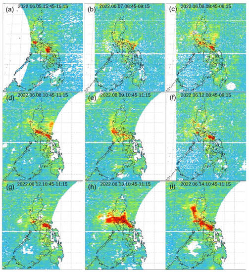
Figure 9.
Total SO2 concentration observed during the eruption of Taal Volcano in the Philippines in June 2022. (a) 5 June, 15:45–16:15, (b) 7 June, 08:45–09:15, (c) 8 June, 08:45–09:15, (d) 8 June, 10:45–11:15, (e) 9 June, 10:45–11:15, (f) 12 June, 08:45–09:15, (g) 12 June, 10:45–11:15, (h) 13 June, 10:45–11:15, and (i) 14 June, 10:45–11:15. Time is expressed in KST.
Figure 10 displays the change in SO2 concentrations at the Taal and Bulusan Volcanoes. The observed data indicate high levels of SO2 emissions during the period of interest. Notably, a temporal offset was observed between the Taal and Bulusan eruptions on 11 June. Furthermore, both volcanoes exhibited elevated SO2 concentrations on 13 and 14 June.
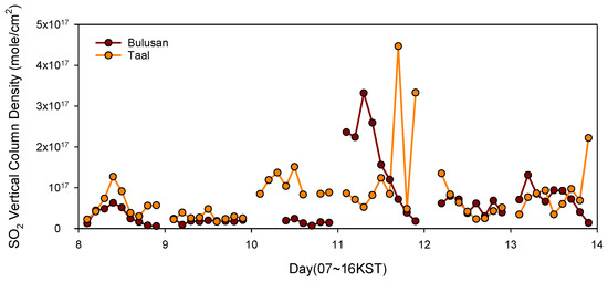
Figure 10.
Temporal variations in the SO2 concentration at the Bulusan and Taal Volcano sites as observed by GEMS.
3.2.3. AOD
According to a previous study [37], when the GEMS AOD algorithm using OMI L1b was compared with the AERONET and OMI algorithms, the r values were 0.83 and 0.86, respectively.
Figure 11 presents the spatial distribution of the seasonal average AOD. In Northeast Asia, Korea, and China, the AOD was low in summer but high in winter. In the Indochina Peninsula region, it was high in spring. These results are consistent with those of a previous study, which reported increased AOD due to biomass burning in the area [38,39,40]. In addition, there were several locations in summer that are not displayed due to the lack of valid data on the Indochina Peninsula. The AOD algorithm, utilizing UV wavelengths, is extremely sensitive to the presence of clouds. Consequently, even minimal cloud coverage presents a substantial obstacle in accurately estimating the AOD; therefore, the AOD could not be calculated because it was not calculated for the Indochina Peninsula, which experiences rainfall during summer.
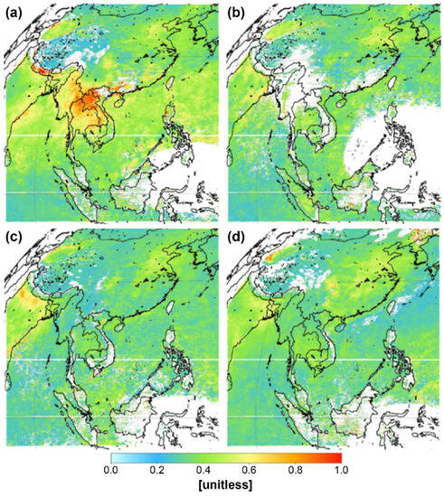
Figure 11.
Full-layer concentration average of the Level 2 aerosol optical depth (AOD) was calculated using spectral information for six wavelengths (354, 388, 412, 443, 477, and 490 nm) observed at 12:45–13:15 (KST): (a) spring (1 March 2021–31 May 2021), (b) summer (1 June 2021–31 August 2021), (c) fall (1 September 2021–30 November 2021), and (d) winter (1 December 2021–28 February 2022).
3.2.4. Formaldehyde
Figure 12 shows the spatial distribution of the monthly median VCD of HCHO obtained by GEMS during April 2021, July 2021, October 2021, and January 2022. The data near the oceans in Southeast Asia, where sunlight is strongly reflected, were disregarded. Similar to other factors, if analyzed separately in Northeast Asia, South Asia, and India, VCD was highest in the mid-latitude regions of Northeast Asia and northern India during July, when the vegetation activity was most active among the four seasons. In the Indochina region, the VCD of HCHO was the highest in April because HCHO was affected by the biomass combustion that occurs during the dry season [53]. Conversely, the equatorial regions of Malaysia and Indonesia showed consistently high HCHO concentrations in spring and summer and higher concentrations in autumn and winter than the other regions.
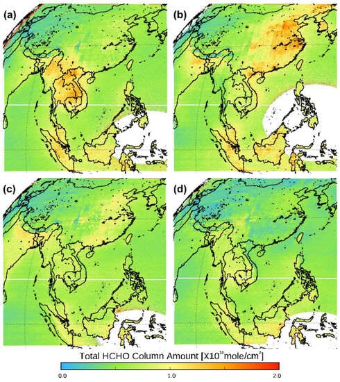
Figure 12.
Spatial distribution of the monthly median vertical column density (VCD) of the HCHO concentrations observed at 12:45–13:15 in (a) April 2021, (b) July 2021, (c) October 2021, and (d) January 2022.
3.2.5. Additional Geostationary Environment Monitoring Spectrometer Products
NIER provides a total of 20 Level 2 products of GEMS including parameters not presented in this study such as single scattering albedo, aerosol type, aerosol effective height, UV index, vitamin D synthesis index, vegetation response index, DNA damage index, surface reflectance, cloud radiation index, cloud effective index, O3 profile, and glyoxal. The NIER provides the observation results after July 2022 sequentially by item [54].
3.3. Validation and Future Implications
3.3.1. Satellite Integrated Joint Air Quality Monitoring
Korea’s Ministry of Environment has conducted intensive air quality observations [12] together with NASA in the United States [13] and is planning to carry out a second campaign for East Asia in 2024 after operating GEMS. In addition, the GEMS Map of Air Pollution (GMAP) campaigns were preliminarily carried out in 2020 and 2021 [55]. Despite the COVID-19 pandemic, NASA, the Max Planck Institute in Europe, the Royal Belgian Institute for Space Aeronomy, and the University of Bremen participated in the GMAP campaign.
The Satellite Integrated Joint Air Quality (SIJAQ) campaign is expected to enable in-depth research on air quality phenomena through general direct observation, terrestrial remote sensing, and wide-area observation in East Asia using GEMS and other instruments onboard LEO satellites such as TROPOMI. In addition, the verification of environmental parameters observed via GEMS will be included, and related procedures such as the recruitment of participating organizations will be implemented before the campaign.
3.3.2. Pandora Asia Network
Pandora is a ground-based observation device for observing direct sunlight and is used to observe air pollutants such as NO2 and verify GEMS products [56,57]. Accordingly, the Korean government is attempting to provide and install Pandora equipment in 13 countries in Asia (Table 4) to analyze the air quality status of each country and participate in the GEMS verification campaign. In addition, a Pandora network for sharing observed data in Asia will be formed to support periodic quality control for accurate data production.
Table 4.
Target countries of the Pandora Asia Network project.
4. Discussion
This study analyzed the reliability of GEMS observations using the pilot data obtained during the test period of GEMS and attempted to establish the base for air quality analysis.
For the reliability analysis of GEMS, the spatial distributions of the solar irradiance observations and Levels 1c and 2 (O3, NO2, SO2, AOD, and HCHO) were displayed and compared with Level 2 for O3 and NO2, and observed by instruments (i.e., OMI, TROPOMI, and OMPS) onboard the LEO satellites. The solar irradiance observation result was attributed to temporal and spatial dependence, which was possibly, in turn, attributed to the position of the Sun. During the spring and autumn equinoxes, the positions of the Sun were the same; thus, the obtained solar irradiance values were similar. However, the Sun was in the north at the summer solstice; thus, irradiance in the northern area (Seoul) was higher than that in the southern area (equator). Similarly, solar irradiance in the southern area was higher than that in the northern area at winter solstice because the Sun was positioned in the south (Figure 6 in Choi et al. [23] illustrates the Sun’s position). This is believed to be due to the change in the angle of incidence of the diffuser of GEMS.
The spatial distributions of O3, NO2, SO2, AOD, and HCHO over East Asia were analyzed for consistency with previous findings [25,26,27,28,29,30,31,32,33,34,35,36,37,38,39,40,41,42]. The VCD of O3 observed via GEMS was similar to that of all existing LEO satellites at a high level in terms of absolute values (errors between GEMS and both satellites are less than ±1 DU) and correlation coefficients (r = 0.90 for OMI vs. GEMS; 0.97 for TROPOMI vs. GEMS). Moreover, a comparison of NO2 observed via GEMS and TROPOMI showed the highest r value in summer (0.83) and the lowest value (0.47) with OMI and OMPS in winter. The absolute value for GEMS was higher than that for LEO satellites (10–38%). However, an in-depth analysis of GEMS observations remains warranted because a previous study [58] reported lower NO2 concentrations via low-orbit satellites than VCDs observed on the ground.
In addition, the diurnal change observed via GEMS was compared with in situ measurements on the ground and analyzed. The maximum value of ground observation for O3 was approximately 3 h later than that of GEMS, whereas for NO2, GEMS was approximately 4 h later. This time difference was attributed to the difference in the vertical altitude at which NO2 and O3 were generated.
Herein, we analyzed the reliability of GEMS using the existing literature and observations of LEO satellites. However, we did not include a comparative analysis with ground-based VCD observations commonly used in the reliability analysis of existing satellites, which is a limitation of this study. Particularly, in situ observations of the ground are not VCDs; hence, direct comparison with GEMS is not possible. Therefore, reliability can be assessed through direct comparison with VCDs measured via MAX-DOAS and Pandora [51,59], similar to the verification of other satellites [57,59,60,61]. Additionally, to verify the vertical concentration profile by GEMS and improve the algorithm, it is necessary to obtain airborne and the sonde data [62,63]. Future studies should conduct ground-based VCD comparative analysis such as the SIJAQ campaign and the establishment of PAN, which can improve algorithms.
5. Conclusions
The pilot operation of GEMS, launched in February 2020, was completed, and the observation data were sequentially released starting from July 2022. The spatial distribution of GEMS observation items (O3, NO2, SO2, AOD, HCHO) was similar to those reported in previous studies. When comparing the GEMS observations with the LEO satellites (OMI, TROPOMI, OMPS), the O3 results were similar, but the NO2 observations from GEMS were higher than those from the LEO satellites.
Due to its operation in the geostationary orbit, GEMS can make multiple observations per day, enabling the monitoring of daily variations in air pollutant concentrations and in-depth analysis of changes in air quality. To analyze the feasibility of this diurnal monitoring method by GEMS, we presented the results of analyzing the VCD values of O3 and NO2 observed over Seoul.
Based on these results, GEMS can be used for the effective analysis of the behavior and impacts of air pollutants. Despite its limitations such as daytime-only observations and low accuracy compared to in situ observations, GEMS has been confirmed as a suitable tool for atmospheric environmental analysis.
Finally, plans are underway to develop strategies to verify and improve the quality of Level 2 data observed via GEMS such as an air quality intensive monitoring campaign (SIJAQ) and the establishment of a ground-based remote sensing network (Pandora Asia Network). These strategies, in conjunction with GEMS, are expected to contribute to the comprehensive analysis of the quality of GEMS observation data and represent a crucial turning point in the analysis and development of countermeasures for the deteriorating atmospheric environment in East Asia [64].
Author Contributions
Conceptualization, W.J.C.; Methodology, K.-J.M.; Software, G.K.; Validation, W.J.C.; Formal analysis, G.K.; Investigation, W.J.C.; Resources, G.K.; Data curation, G.K.; Writing—original draft preparation, K.-J.M.; Writing—review and editing, W.J.C.; Visualization, G.K.; Supervision, W.J.C.; Project administration, D.L.; Funding acquisition, D.L. All authors have read and agreed to the published version of the manuscript.
Funding
This research was funded by the National Institute of Environmental Research, funded by the Ministry of Environment of the Republic of Korea (Grant number: NIER-2018-01-01-020).
Institutional Review Board Statement
Not applicable.
Informed Consent Statement
Not applicable.
Data Availability Statement
Efforts were made to use the latest data from March 2021 to February 2022, when GEMS was operated at the Environmental Satellite Center (ESC) of the National Institute of Environmental Research. Furthermore, all data used in this study were based on local standard time (LST, KST, UTC + 9). Data for OMI, TROPOMI, and OMPS provided by NASA were used from March 2021 to February 2022 [http://disc.gsfc.nasa.gov (accessed on 18 September, 2023)]. For the ground observation data of O3 and NO2, the averaged values of the observation data for which QA/QC was completed in 25 districts of Seoul were used [http://airkorea.or.kr (accessed on 18 September 2023)].
Acknowledgments
We thank those who participated in the stabilization process during the development and pilot operation of the GEMS hardware and algorithms and all those involved in the data generation of the GEMS. In particular, we express our sincere gratitude to the ESC, GEMS Science Team, Korea Aerospace Research Institute, Ministry of Environment of the Republic of Korea, and Ministry of Science and ICT (Information and Communication Technologies). Additionally, we express our gratitude to Professor Ja-Ho Koo from Yonsei University for providing us with the O3 total column concentration data observed in Seoul.
Conflicts of Interest
The authors declare no conflict of interest.
References
- Loomis, D.; Grosse, Y.; Lauby-Secretan, B.; El Ghissassi, F.; Bouvard, V.; Benbrahim-Tallaa, L.; Guha, N.; Baan, R.; Mattock, H.; Straif, K.; et al. The carcinogenicity of outdoor air pollution. Lancet Oncol. 2013, 14, 1262–1263. [Google Scholar] [CrossRef] [PubMed]
- Ayres, J.G.; Borm, P.; Cassee, F.R.; Castranova, V.; Donaldson, K.; Ghio, A.; Harrison, R.M.; Hider, R.; Kelly, F.; Kooter, I.M.; et al. Evaluating the toxicity of airborne particulate matter and nanoparticles by measuring oxidative stress potential—A workshop report and consensus statement. Inhal. Toxicol. 2008, 20, 75–99. [Google Scholar] [CrossRef] [PubMed]
- Kim, K.H.; Kabir, E.; Kabir, S. A review on the human health impact of airborne particulate matter. Environ. Int. 2015, 74, 136–143. [Google Scholar] [CrossRef] [PubMed]
- Pope, C.A., III; Burnett, R.T.; Thurston, G.D.; Thun, M.J.; Calle, E.E.; Krewski, D.; Godleski, J.J. Cardiovascular mortality and long-term exposure to particulate air pollution: Epidemiological evidence of general pathophysiological pathways of disease. Circulation 2004, 109, 71–77. [Google Scholar] [CrossRef]
- Brook, R.D.; Rajagopalan, S.; Pope, C.A., III; Brook, J.R.; Bhatnagar, A.; Diez-Roux, A.V.; Holguin, F.; Hong, Y.; Luepker, R.V.; Mittleman, M.A.; et al. Particulate matter air pollution and cardiovascular disease: An update to the scientific statement from the American Heart Association. Circulation 2010, 121, 2331–2378. [Google Scholar] [CrossRef]
- World Health Organization 2023 Newsroom. Available online: https://www.who.int/news-room/headlines (accessed on 7 February 2023).
- Sillman, S. The relation between ozone, NOx and hydrocarbons in urban and polluted rural environments. Atmos. Environ. 1999, 33, 1821–1845. [Google Scholar] [CrossRef]
- Jones, A.M.; Harrison, R.M.; Baker, J. The wind speed dependence of the concentrations of airborne particulate matter and NOx. Atmos. Environ. 2010, 44, 1682–1690. [Google Scholar] [CrossRef]
- Takeuchi, M.; Berkemeier, T.; Eris, G.; Ng, N.L. Non-linear effects of secondary organic aerosol formation and properties in multi-precursor systems. Nat. Commun. 2022, 13, 7883. [Google Scholar] [CrossRef]
- Kim, B.; Bae, C.; Kim, H.C.; Kim, E.; Kim, S. Spatially and chemically resolved source apportionment analysis: Case study of high particulate matter event. Atmos. Environ. 2017, 162, 55–70. [Google Scholar] [CrossRef]
- Kim, H.C.; Kim, E.; Bae, C.; Cho, J.H.; Kim, B.; Kim, S. Regional contributions to particulate matter concentration in the Seoul metropolitan area, South Korea: Seasonal variation and sensitivity to meteorology and emissions inventory. Atmos. Chem. Phys. 2017, 17, 10315–10332. [Google Scholar] [CrossRef]
- Choi, J.; Park, R.J.; Lee, H.; Lee, S.; Jo, D.S.; Jeong, J.I.; Henze, D.K.; Woo, J.; Ban, S.; Lee, M.; et al. Impacts of local vs. trans-boundary emissions from different sectors on PM2.5 exposure in South Korea during the KORUS-AQ campaign. Atmos. Environ. 2019, 203, 196–205. [Google Scholar] [CrossRef]
- Uranishi, K.; Ikemori, F.; Shimadera, H.; Kondo, A.; Sugata, S. Impact of field biomass burning on local pollution and long-range transport of PM2.5 in NorthEast Asia. Environ. Pollut. 2019, 244, 414–422. [Google Scholar] [CrossRef] [PubMed]
- Chang, J.C.; Hanna, S.R. Air quality model performance evaluation. Meteorol. Atmos. Phys. 2004, 87, 167–196. [Google Scholar] [CrossRef]
- Choi, W.J.; Jung, B.; Lee, D.; Kang, H.; Kim, H.; Hong, H. An investigation into the effect of emissions from industrial complexes on air quality in the Ulsan metropolitan city utilizing trace components in PM2.5. Appl. Sci. 2021, 11, 10003. [Google Scholar] [CrossRef]
- Crawford, J.H.; Ahn, J.Y.; Al-Saadi, J.; Chang, L.; Emmons, L.K.; Kim, J.; Lee, G.; Park, J.H.; Park, R.J.; Woo, J.H.; et al. The Korea-United States Air Quality (KORUS-AQ) field study. Elementa 2021, 9, 00163. [Google Scholar] [CrossRef] [PubMed]
- Bovensmann, H.; Burrows, J.P.; Buchwitz, M.; Frerick, J.; Noël, S.; Rozanov, V.V.; Chance, K.V.; Goede, A.P.H. SCIAMACHY: Mission objectives and measurement modes. J. Atmos. Sci. 1999, 56, 127–150. [Google Scholar] [CrossRef]
- Levelt, P.F.; van den Oord, G.H.J.; Dobber, M.R.; Malkki, A.; Visser, H.; de Vries, J.; Stammes, P.; Lundell, J.O.V.; Saari, H. The ozone monitoring instrument. IEEE Trans. Geosci. Remote Sens. 2006, 44, 1093–1101. [Google Scholar] [CrossRef]
- Martin, R.V. Satellite remote sensing of surface air quality. Atmos. Environ. 2008, 42, 7823–7843. [Google Scholar] [CrossRef]
- Veefkind, J.P.; Aben, I.; McMullan, K.; Förster, H.; De Vries, J.; Otter, G.; Claas, J.; Eskes, H.J.; De Haan, J.F.; Kleipool, Q.; et al. TROPOMI on the ESA Sentinel-5 Precursor: A GMES mission for global observations of the atmospheric composition for climate, air quality and ozone layer applications. Remote Sens. Environ. 2012, 120, 70–83. [Google Scholar] [CrossRef]
- Flynn, L.; Long, C.; Wu, X.; Evans, R.; Beck, C.T.; Petropavlovskikh, I.; McConville, G.; Yu, W.; Zhang, Z.; Niu, J.; et al. Performance of the ozone mapping and profiler suite (OMPS) products. J. Geophys. Res. Atmos. 2014, 119, 6181–6195. [Google Scholar] [CrossRef]
- Zoogman, P.; Liu, X.; Suleiman, R.M.; Pennington, W.F.; Flittner, D.E.; Al-Saadi, J.A.; Hilton, B.B.; Nicks, D.K.; Newchurch, M.J.; Carr, J.L.; et al. Tropospheric emissions: Monitoring of pollution (TEMPO). J. Quant. Spectrosc. Radiat. Transf. 2017, 186, 17–39. [Google Scholar] [CrossRef] [PubMed]
- Choi, W.J.; Moon, K.J.; Yoon, J.; Cho, A.; Kim, S.K.; Lee, S.; Ko, D.H.; Kim, J.; Ahn, M.H.; Kim, D.R.; et al. Introducing the geostationary environment monitoring spectrometer. J. Appl. Remote Sens. 2018, 12, 044005. [Google Scholar] [CrossRef]
- Kim, J.; Jeong, U.; Ahn, M.; Kim, J.H.; Park, R.J.; Lee, H.; Song, C.H.; Choi, Y.; Lee, K.; Yoo, J.; et al. New era of air quality monitoring from space: Geostationary environment monitoring spectrometer (GEMS). Bull. Am. Meteorol. Soc. 2020, 101, E1–E22. [Google Scholar] [CrossRef]
- Chubarova, N.E.; Pastukhova, A.S.; Zhdanova, E.Y.; Volpert, E.V.; Smyshlyaev, S.P.; Galin, V.Y. Effects of ozone and clouds on temporal variability of surface UV radiation and UV resources over Northern Eurasia derived from measurements and modeling. Atmosphere 2020, 11, 59. [Google Scholar] [CrossRef]
- Baruah, U.D.; Robeson, S.M.; Saikia, A.; Mili, N.; Sung, K.; Chand, P. Spatio-temporal characterization of tropospheric ozone and its precursor pollutants NO2 and HCHO over South Asia. Sci. Total Environ. 2022, 809, 151135. [Google Scholar] [CrossRef]
- Liu, N.; Lin, W.; Ma, J.; Xu, W.; Xu, X. Seasonal variation in surface ozone and its regional characteristics at global atmosphere watch stations in China. J. Environ. Sci. 2019, 77, 291–302. [Google Scholar] [CrossRef] [PubMed]
- Wei, J.; Li, Z.; Li, K.; Dickerson, R.R.; Pinker, R.T.; Wang, J.; Liu, X.; Sun, L.; Xue, W.; Cribb, M. Full-coverage mapping and spatiotemporal variations of ground-level ozone (O3) pollution from 2013 to 2020 across China. Remote Sens. Environ. 2022, 270, 112775. [Google Scholar] [CrossRef]
- Li, J.; Nagashima, T.; Kong, L.; Ge, B.; Yamaji, K.; Fu, J.S.; Wang, X.; Fan, Q.; Itahashi, S.; Lee, H.J.; et al. Model evaluation and intercomparison of surface-level ozone and relevant species in East Asia in the context of MICS-Asia Phase III—Part 1: Overview. Atmos. Chem. Phys. 2019, 19, 12993–13015. [Google Scholar] [CrossRef]
- Marvin, M.R.; Palmer, P.I.; Latter, B.G.; Siddans, R.; Kerridge, B.J.; Latif, M.T.; Khan, M.F. Photochemical environment over Southeast Asia primed for hazardous ozone levels with influx of nitrogen oxides from seasonal biomass burning. Atmos. Chem. Phys. 2021, 21, 1917–1935. [Google Scholar] [CrossRef]
- Uno, I.; He, Y.; Ohara, T.; Yamaji, K.; Kurokawa, J.-I.; Katayama, M.; Wang, Z.; Noguchi, K.; Hayashida, S.; Richter, A.; et al. Systematic analysis of interannual and seasonal variations of model-simulated tropospheric NO2 in Asia and comparison with GOME-satellite data. Atmos. Chem. Phys. 2007, 7, 1671–1681. [Google Scholar] [CrossRef]
- Kim, D.R.; Lee, J.B.; Keun Song, C.K.; Kim, S.Y.; Ma, Y.L.; Lee, K.M.; Cha, J.S.; Lee, S.D. Temporal and spatial distribution of tropospheric NO2 over Northeast Asia using OMI data during the years 2005–2010. Atmos. Pollut. Res. 2015, 6, 768–776. [Google Scholar] [CrossRef]
- Lin, C.A.; Chen, Y.C.; Liu, C.Y.; Chen, W.T.; Seinfeld, J.H.; Chou, C.C.-K. Satellite-derived correlation of SO2, NO2, and aerosol optical depth with meteorological conditions over East Asia from 2005 to 2015. Remote Sens. 2019, 11, 1738. [Google Scholar] [CrossRef]
- Van Der A, R.J.; Eskes, H.J.; Boersma, K.F.; Van Noije, T.P.C.; Van Roozendael, M.; De Smedt, I.; Peters, D.H.M.U.; Meijer, E.W. Trends, seasonal variability and dominant NOx source derived from a ten year record of NO2 measured from space. J. Geophys. Res. 2008, 133, D04302. [Google Scholar] [CrossRef]
- Duncan, B.N.; Lamsal, L.N.; Thompson, A.M.; Yoshida, Y.; Lu, Z.; Streets, D.G.; Hurwitz, M.M.; Pickering, K.E. A space-based, high-resolution view of notable changes in urban NOx pollution around the world (2005–2014). J. Geophys. Res. Atmos. 2016, 121, 976–996. [Google Scholar] [CrossRef]
- ul-Haq, Z.; Tariq, S.; Ali, M. Spatiotemporal patterns of correlation between atmospheric nitrogen dioxide and aerosols over South Asia. Meteorol. Atmos. Phys. 2017, 129, 507–527. [Google Scholar] [CrossRef]
- Kim, M.; Kim, J.; Torres, O.; Ahn, C.; Kim, W.; Jeong, U.; Go, S.; Liu, X.; Moon, K.J.; Kim, D.-R. Optimal estimation-based algorithm to retrieve aerosol optical properties for GEMS measurements over Asia. Remote Sens. 2018, 10, 162. [Google Scholar] [CrossRef]
- Nguyen, T.T.N.; Pham, H.V.; Lasko, K.; Bui, M.T.; Laffly, D.; Jourdan, A.; Bui, H.Q. Spatiotemporal analysis of ground and satellite-based aerosol for air quality assessment in the Southeast Asia region. Environ. Pollut. 2019, 255, 113106. [Google Scholar] [CrossRef]
- Lin, N.-H.; Tsay, S.-C.; Maring, H.B.; Yen, M.-C.; Sheu, G.-R.; Wang, S.-H.; Chi, K.H.; Chuang, M.-T.; Ou-Yang, C.-F.; Fu, J.S.; et al. An overview of regional experiments on biomass burning aerosols and related pollutants in Southeast Asia: From BASE-ASIA and the Dongsha Experiment to 7-SEAS. Atmos. Environ. 2013, 78, 1–19. [Google Scholar] [CrossRef]
- Wang, S.-H.; Welton, E.J.; Holben, B.N.; Tsay, S.-C.; Lin, N.-H.; Giles, D.; Stewart, S.A.; Janjai, S.; Nguyen, X.A.; Hsiao, T.-C.; et al. Vertical distribution and columnar optical properties of springtime biomass-burning aerosols over Northern Indochina during 2014 7-SEAS Campaign. Aerosol Air Qual. Res. 2015, 15, 2037–2050. [Google Scholar] [CrossRef]
- Ge, C.; Wang, J.; Carn, S.; Yang, K.; Ginoux, P.; Krotkov, N. Satellite-based global volcanic SO2 emissions and sulfate direct radiative forcing during 2005–2012. J. Geophys. Res. Atmos. 2016, 121, 3446–3464. [Google Scholar] [CrossRef]
- Flower, V.J.B.; Kahn, R.A. Twenty years of NASA-EOS multi-sensor satellite observations at Kīlauea volcano (2000–2019). J. Volcanol. Geotherm. Res. 2021, 415, 107247. [Google Scholar] [CrossRef]
- Coste, P.; Larnaudie, F.; Luquet, P.; Heo, H.; Jung, J.; Kang, G.; Shin, S.; Yong, S.; Park, Y.-J. Development of the New Generation of Geostationary Ocean Color Imager. In Proceedings of the International Conference on Space Optics–ICSO 2016, Biarritz, France, 25 September 2017; SPIE: Bellingham, WA, USA, 2017; Volume 10562, pp. 98–106. [Google Scholar] [CrossRef][Green Version]
- Kang, M.; Ahn, M.; Liu, X.; Jeong, U.; Kim, J. Spectral calibration algorithm for the geostationary environment monitoring spectrometer (GEMS). Remote Sens. 2020, 12, 2846. [Google Scholar] [CrossRef]
- Choi, H.; Lee, K.; Seo, J.; Bae, J. The influence of atmospheric composition on polarization in the GEMS spectral region. Asia-Pac. J. Atmos. Sci. 2021, 57, 587–603. [Google Scholar] [CrossRef]
- Haffner, D.P.; McPeters, R.D.; Bhartia, P.K.; Labow, G.J. The TOMS v9 algorithm for OMPS nadir mapper total ozone: An enhanced design that ensures data continuity. In AGU Fall Meeting Abstracts; American Geophysical Union: San Francisco, CA, USA, 2015. [Google Scholar]
- Spurr, R. LIDORT and VLIDORT: Linearized pseudo-spherical scalar and vector discrete ordinate radiative transfer models for use in remote sensing retrieval problems. In Light Scattering Reviews 3; Springer: Berlin/Heidelberg, Germany, 2008; pp. 229–275. [Google Scholar] [CrossRef]
- Rodgers, C.D. Inverse Methods for Atmospheric Sounding-Theory and Practice Series: Series on Atmospheric Oceanic and Planetary Physics; Rodgers, C.D., Ed.; World Scientific Publishing Co. Pte. Ltd.: Singapore, 2000; Volume 2, ISBN 978-981-281-371-8. [Google Scholar]
- Kwon, H.A.; Park, R.J.; González Abad, G.; Chance, K.; Kurosu, T.P.; Kim, J.; De Smedt, I.; Van Roozendael, M.; Peters, E.; Burrows, J. Description of a formaldehyde retrieval algorithm for the geostationary environment monitoring spectrometer (GEMS). Atmos. Meas. Tech. 2019, 12, 3551–3571. [Google Scholar] [CrossRef]
- Bak, J.; Baek, K.H.; Kim, J.H.; Liu, X.; Kim, J.; Chance, K. Cross-evaluation of GEMS tropospheric ozone retrieval performance using OMI data and the use of an ozonesonde dataset over East Asia for validation. Atmos. Meas. Tech. 2019, 12, 5201–5215. [Google Scholar] [CrossRef]
- Hönninger, G.; von Friedeburg, C.; Platt, U. Multi axis differential optical absorption spectroscopy (MAX-DOAS). Atmos. Chem. Phys. 2004, 4, 231–254. [Google Scholar] [CrossRef]
- Park, J.; Choi, W.; Lee, H.-M.; Park, R.J.; Kim, S.-Y.; Yu, J.-A.; Lee, D.-W.; Lee, H. Effect of error in SO2 slant column density on the accuracy of SO2 transport flow rate estimates based on GEMS synthetic radiances. Remote Sens. 2021, 13, 3047. [Google Scholar] [CrossRef]
- Baek, K.H.; Kim, J.H.; Park, R.J.; Chance, K.; Kurosu, T.P. Validation of OMI HCHO data and its analysis over Asia. Sci. Total Environ. 2014, 490, 93–105. [Google Scholar] [CrossRef]
- Environmental Satellite Center (2022) Image View. Available online: https://nesc.nier.go.kr/product/vie (accessed on 18 September 2023).
- Chang, L.S.; Kim, D.; Hong, H.; Kim, D.R.; Yu, J.; Lee, K.; Lee, H.; Kim, D.; Hong, J.; Jo, H.-Y.; et al. Evaluation of correlated Pandora column observations and in situ surface air quality measurements during GMAP campaign. Atmos. Chem. Phys. 2022, 22, 10703–10720. [Google Scholar] [CrossRef]
- Tzortziou, M.; Herman, J.R.; Cede, A.; Loughner, C.P.; Abuhassan, N.; Naik, S. Spatial and temporal variability of ozone and nitrogen dioxide over a major urban estuarine ecosystem. J. Atmos. Chem. 2015, 72, 287–309. [Google Scholar] [CrossRef]
- Herman, J.; Cede, A.; Spinei, E.; Mount, G.; Tzortziou, M.; Abuhassan, N. NO2 column amounts from ground-based Pandora and MFDOAS spectrometers using the direct-sun DOAS technique: Intercomparisons and application to OMI validation. J. Geophys. Res. 2009, 114, D13307. [Google Scholar] [CrossRef]
- Pinardi, G.; Van Roozendael, M.; Hendrick, F.; Theys, N.; Abuhassan, N.; Bais, A.; Boersma, F.; Cede, A.; Chong, J.; Donner, S.; et al. Validation of tropospheric NO2 column measurements of GOME-2A and OMI using MAX-DOAS and direct sun network observations. Atmos. Meas. Tech. 2020, 13, 6141–6174. [Google Scholar] [CrossRef]
- Wang, C.; Wang, T.; Wang, P.; Rakitin, V. Comparison and validation of TROPOMI and OMI NO2 observations over China. Atmosphere 2020, 11, 636. [Google Scholar] [CrossRef]
- Herman, J.; Spinei, E.; Fried, A.; Kim, J.; Kim, J.; Kim, W.; Cede, A.; Abuhassan, N.; Segal-Roenhaimer, M. NO2 and HCHO measurements in Korea from 2012 to 2016 from Pandora spectrometer instruments compared with OMI retrievals and with aircraft measurements during the KORUS-AQ campaign. Atmos. Meas. Tech. 2018, 11, 4583–4603. [Google Scholar] [CrossRef]
- Ialongo, I.; Virta, H.; Eskes, H.; Hovila, J.; Douros, J. Comparison of TROPOMI/Sentinel-5 Precursor NO2 observations with ground-based measurements in Helsinki. Atmos. Meas. Tech. 2020, 13, 205–218. [Google Scholar] [CrossRef]
- Pittman, J.V.; Pan, L.L.; Wei, J.C.; Irion, F.W.; Liu, X.; Maddy, E.S.; Barnet, C.D.; Chance, K.; Gao, R. Evaluation of AIRS, IASI, and OMI ozone profile retrievals in the extratropical tropopause region using in situ aircraft measurements. J. Geophys. Res. 2009, 114, D24109. [Google Scholar] [CrossRef]
- Hubert, D.; Heue, K.P.; Lambert, J.C.; Verhoelst, T.; Allaart, M.; Compernolle, S.; Cullis, P.D.; Dehn, A.; Félix, C.; Johnson, B.J.; et al. TROPOMI tropospheric ozone column data: Geophysical assessment and comparison to ozonesondes, GOME-2B and OMI. Atmos. Meas. Tech. 2021, 14, 7405–7433. [Google Scholar] [CrossRef]
- Chen, X.; Jiang, Z.; Shen, Y.; Li, R.; Fu, Y.; Liu, J.; Han, H.; Liao, H.; Cheng, X.; Jones, D.B.A.; et al. Chinese regulations are working—Why is surface ozone over industrialized areas still high? Applying lessons from Northeast US air quality evolution. Geophys. Res. Lett. 2021, 48, e2021GL092816. [Google Scholar] [CrossRef]
Disclaimer/Publisher’s Note: The statements, opinions and data contained in all publications are solely those of the individual author(s) and contributor(s) and not of MDPI and/or the editor(s). MDPI and/or the editor(s) disclaim responsibility for any injury to people or property resulting from any ideas, methods, instructions or products referred to in the content. |
© 2023 by the authors. Licensee MDPI, Basel, Switzerland. This article is an open access article distributed under the terms and conditions of the Creative Commons Attribution (CC BY) license (https://creativecommons.org/licenses/by/4.0/).