Abstract
Based on the hourly ERA5 reanalysis dataset of the European Centre for Medium-Range Weather Forecasts (ECMWF) from 1 January 1979 to 31 December 2019, the climatology of the planetary boundary layer height (PBLH) in Jiangsu, China, is studied. The PBLH based on ERA5 is verified by using radiosonde data, and the results show that the PBLH based on ERA5 fits very well with the PBLH diagnosed by the radiosonde data. Overall, the daytime average PBLH is between 700 and 1200 m, which is higher in the north and lower in the south. It is between 100 and 400 m at night, and it is lower in the north and higher in the south. The PBLH exhibits complex spatiotemporal variation. In the daytime, the PBLH in inland areas is highest in spring, followed by fall and summer, and lowest in winter. At night, the seasonal variation in the PBLH is less obvious. The seasonal variation in the PBLH in coastal areas is higher in fall and winter and lower in spring and summer. The PBLH shows an obvious diurnal cycle, usually reaching its peak at 14:00 (LST) or 15:00 (LST). The diurnal cycle of the PBLH is significantly positively correlated with the near-surface temperature and wind speed and significantly negatively correlated with the relative humidity and lower tropospheric stability. Over these 41 years, the daytime PBLH has increased significantly in most areas. The increase in the PBLH can be attributed to the increase in near-surface temperature and the decrease in near-surface relative humidity and lower tropospheric stability.
1. Introduction
The planetary boundary layer (PBL) is the low atmosphere close to the Earth’s surface, is directly affected by the forced action of the Earth’s surface, with a height up to several kilometers, and is the main area of human activity [1]. The Earth’s surface exchanges heat, momentum, water vapor, and chemicals with the free atmosphere through the PBL. Since the PBL involves many processes, such as convective activity, turbulent mixing, low-layer cloud formation, pollutant diffusion, and surface energy budget, the PBL plays a key role in many aspects, such as weather, climate, and air pollution [2]. The planetary boundary layer height (PBLH) is an important parameter for characterizing the structural characteristics of the PBL. It determines the vertical degree of turbulent mixing, convective transport, and pollutant diffusion in the PBL and strongly influences the development and evolution of convective activity [3,4,5]. The PBLH is one of the most important parameters in weather forecasting, climate and air quality forecasting models [6,7,8].
Currently, there are many datasets and methods to obtain the PBLH. Among them, radiosonde datasets are one of the most widely used datasets. The radiosonde can obtain the vertical profiles of physical quantities such as temperature, humidity, wind direction, and wind speed and diagnose the PBLH through the parcel method, potential temperature gradient method, relative humidity gradient method, bulk Richardson number method, and so on [9]. In addition to radiosonde data, remote sensing data can also be used to estimate the PBLH, including lidar [10,11], wind profiler radar [12,13], ceilometer [14,15], etc. Radar can achieve continuous observations, thus obtaining high-temporal-resolution data. With the development of satellite remote sensing technology, GPS radio occultation data and cloud-aerosol lidar data are also used in PBL studies [16,17,18,19]. Although the resolution is relatively low, they can expand the spatial coverage of observations. In addition to the above sounding data, reanalysis data and model data are also commonly used in PBLH studies [20,21,22]. They have the advantages of high temporal and spatial resolutions and can realize long-term and large-scale PBLH climatology studies.
Climatology research on the PBLH began with the work of Holzworth [23], who first used radiosonde data to obtain the characteristics of the height of the mixed layer in the United States. Later, Liu and Liang [24] studied the diurnal cycle climatology of the PBLH using radiosonde data from 14 stations around the world. Seidel et al. [20] used radiosonde data, reanalysis data, and simulated data to analyze the diurnal and seasonal variations in the PBLH in the United States and Europe and obtained more climatic characteristics of the PBLH. At present, many scholars have conducted research on the PBLH in different regions of China through different datasets and methods [19,25,26,27]. Zhao et al. [28] studied the characteristics of the PBLH in Northwest China using radiosonde data from 2015 to 2016. Guo et al. [26] studied the PBLH climatology in China based on radiosonde data from 2011 to 2015. However, due to the difficulty of PBL observation, it is difficult to obtain long-term, high-temporal-resolution observational data, resulting in most studies being confined to specific locations or datasets with short durations and low resolutions. Therefore, it is still necessary to use reanalysis data for long-term PBLH climatology studies. Seidel et al. [20] showed that reanalysis data such as ERA-Interim and NCAR-CAM5 could reproduce the spatial and seasonal distributions of the PBLH well. Zhao et al. [29] studied the variation in the PBLH in arid and semiarid regions of East Asia over 110 years through ERA-20C reanalysis data. von Engeln et al. [21] studied global PBLH climatology from 1990 to 2009 using ERA-Interim reanalysis data. ERA5 is the latest reanalysis data from the European Centre for Medium-Range Weather Forecasts (ECMWF). Altabakash et al. [30] studied the PBLH of the Korean Peninsula using ERA5 data and noted that the PBLH obtained from ERA5 data is very consistent with the PBLH obtained from radiosonde and GPS radio occultation data. We use PBLH data from ERA5 to carry out our research. First, we use radiosonde data to verify ERA5 data and then use ERA5 data to study the climatology of the PBLH, which will provide some reference for the application of ERA5 data and the study of the PBLH in weather forecasting, climate prediction, and air quality forecasting in the future.
In recent years, the temporal variation trend of the PBLH has been widely studied by scholars [27,31,32]. A study by Yang et al. [33] used ground-based lidar data and noted that the PBLH in Hong Kong showed a downward trend from 2004 to 2009. Zhang et al. [31] used radiosonde data from 25 sites in Europe from 1973 to 2010 to reveal the increasing trend of the PBLH and attributed it to the decrease in near-surface relative humidity and the increase in near-surface temperature. A recent study showed that the PBLH in China experienced a dramatic mutation in 2004, but the trend varied from place to place [27]. Obviously, previous studies have shown that the temporal variation trend of the PBLH may vary due to different data, methods, or study locations. Also, a study focused on the Jiangsu region is rare. It is necessary to study the long-term temporal variation trend of the PBLH.
Located in the eastern coastal area of China, Jiangsu Province is China’s second-largest economic province, with a dense population and rapid industrial development and urbanization. The PBL is the main area of human activity. The meteorological conditions and atmospheric environment in the PBL have an important influence on human life and health. The PBLH determines the atmospheric environmental capacity and is one of the important factors affecting the transportation and diffusion of pollutants. At present, there have been few studies on the PBLH in Jiangsu. Based on the ECMWF ERA5 reanalysis dataset, this paper studies the climatic characteristics of the PBLH in Jiangsu and its relationship with meteorological factors, analyzes the physical mechanisms affecting the development of the PBL, and reveals the long-term variation trend and causes of the PBLH.
The rest of the paper is arranged as follows: Section 2 introduces the data and methods used; Section 3 verifies the PBLH based on ERA5; Section 4 analyzes the climatic characteristics of the PBLH in Jiangsu and its relationship with meteorological factors and analyzes the long-term trend and causes of the PBLH; and Section 5 presents a summary and discussion.
2. Data and Methods
2.1. Data
2.1.1. ERA5 Reanalysis Data
ERA5 reanalysis data are the fifth-generation reanalysis data of the global climate and weather from the European Centre for Medium-Range Weather Forecasts (ECMWF) and the latest generation reanalysis data of the ECMWF. Reanalysis combines model data with observations from across the world, including satellite and radiosonde datasets and various observational datasets from the World Meteorological Organization’s Global Telecommunication System (GTS), into a globally complete and consistent dataset using the laws of physics. This principle, called data assimilation, is based on the method used by numerical weather prediction centers, where every so many hours (12 h at ECMWF), a previous forecast is combined with newly available observations in an optimal way to produce a new best estimate of the state of the atmosphere, called analysis, from which an updated, improved forecast is issued. Reanalysis works in the same way, but at reduced resolution to allow for the provision of a dataset spanning back several decades. Reanalysis does not have the constraint of issuing timely forecasts, so there is more time to collect observations and, by going further back in time, allows for the ingestion of improved versions of the original observations, which all benefit the quality of the reanalysis product. The ERA5 data cover the entire globe, with a horizontal resolution of 0.25° × 0.25° grid, a vertical resolution of 37 standard pressure layers, and an hourly temporal resolution. In this paper, ERA5 boundary layer height data are used to study the climatic characteristics of the planetary boundary layer height in Jiangsu. The selected time range is from 1979 to 2019, a total of 41 years. In addition, to study the relationship between the PBLH and meteorological factors, data such as 2 m temperature, 10 m wind speed, and near-surface relative humidity (replaced by relative humidity at 1000 hPa) from ERA5 are used, as well as surface pressure and 700 hPa temperature data, which are used to calculate lower tropospheric stability (defined as the potential temperature difference between 700 hPa and the surface [34]).
2.1.2. Radiosonde Data
We used radiosonde data in Jiangsu to verify the PBLH based on ERA5. The selected radiosonde data are obtained from the radiosonde network of the China Meteorological Administration (CMA). Since 2002, the CMA has been upgrading its radiosonde system by using an L-band radar sounding system that combines a secondary wind-measuring radar and a GTS1 digital electronic radiosonde. The system provides high vertical resolution (second-level) profile data, including wind direction, wind speed, temperature, and pressure. By 2010, the L-band sounding system had been applied to 120 radiosonde stations across China. The radiosonde data used in this paper are the L-band conventional sounding data (twice daily: 08:00, 20:00, LST) at Xuzhou Station, Sheyang Station, and Nanjing Station in Jiangsu from 1 January 2010 to 31 December 2019, and include temperature, pressure, wind direction, wind speed, and other conventional meteorological elements. The locations of the three stations are shown in Figure 1. In total, we made use of 21,588 profiles at the three stations, including 3600 profiles at 08:00 (LST) and 3600 profiles at 20:00 (LST) at Xuzhou Station, 3595 profiles at 0800 (LST) and 3600 profiles at 2000 (LST) at Sheyang Station, and 3591 profiles at 0800 (LST) and 3602 profiles at 2000 (LST) at Nanjing Station.
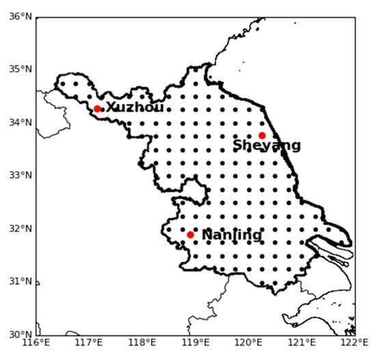
Figure 1.
Spatial distribution of the radiosonde sounding sites (red dots) and ERA5 grids (black dots) over Jiangsu, China.
2.2. PBLH Diagnosis Method
There are many methods to diagnose the PBLH, and the commonly used methods include the potential temperature gradient method [2,35], parcel method [36,37], relative humidity gradient method [21], specific humidity gradient method [21], refractive index gradient method [35,38], and Richardson number method [20,31]. Seidel et al. [9,20] compared and evaluated different diagnostic methods and confirmed that the Richardson number method is more suitable for the diagnosis of the PBLH in large-volume datasets, and this method is suitable for both the stable boundary layer (SBL) and convective boundary layer (CBL). Therefore, in this paper, we choose the Richardson number method to diagnose the PBLH. The Richardson number method determines the PBLH at which the bulk Richardson number first reaches the critical value. Referring to the study of Sicard et al. [39], the formula for calculating the bulk Richardson number (Ri) is as follows:
where g is the gravitational acceleration, z0 is the surface altitude, θ is the potential temperature, and u and v are the zonal wind and meridional wind components, respectively. Previous theories and studies have shown that laminar flow is unstable when the bulk Richardson number Ri is less than the critical value (~0.25) [1]. Guo et al. [26] determined the critical value as 0.25 in their study and noted that the uncertainty caused by the selection of the critical value (0.2, 0.25, and 0.3) is very small. Therefore, in this paper, the critical value is determined as 0.25, and the height when the bulk Richardson number Ri first reaches 0.25 is determined as the PBLH.
2.3. Trend Analysis Method
Following the method used by Guo et al. [27], Sen’s slope estimator [40] is selected to calculate the trend here. The trend is determined as the median of the slopes between all paired values, which is calculated as follows:
where and represent the ith and jth values in the time series of X, respectively. The median is the 50% value of the total datasets. Compared with linear regression, Sen’s slope is less sensitive to outliers. In addition, the nonparametric Mann–Kendall statistical test [41,42] is used to determine the 95% confidence level.
3. Data Validation
The accuracy of some general variables in ERA5 data has been confirmed in some studies [30,43], but the quality of the PBLH in these data has not been verified. To use this dataset to study the characteristics of the PBLH in Jiangsu, the first problem we need to solve is to evaluate the accuracy of the PBLH. In this paper, the PBLH diagnosed by radiosonde data from Xuzhou, Sheyang, and Nanjing stations is used to evaluate the PBLH based on ERA5. To compare the two kinds of PBLH, first, the ERA5 data are sampled at nine grid points centered on the radiosonde position, and then the arithmetic mean is calculated. Second, to maintain consistency with the time of radiosonde data, ERA5 data were sampled at 08:00 (LST) and 20:00 (LST) from 2010 to 2019.
Figure 2 shows the scatter plots of the ERA5 PBLH and the PBLH diagnosed by the radiosonde data from the Xuzhou, Sheyang, and Nanjing stations. At Xuzhou Station, the correlation coefficient between the ERA5 and radiosonde datasets is 0.81 at 08:00 (Figure 2a), and the PBLHs of the two datasets have very good agreement. At 20:00 (Figure 2d), the correlation coefficient between these two is 0.71, and the root mean square error is 198 m. Compared with the radiosonde data, ERA5 generally underestimates the PBLH by 84 m on average. The scatter plots of Sheyang Station show that the correlation coefficient between the ERA5 and radiosonde datasets at 08:00 (Figure 2b) is 0.77, and the root mean square error is 208 m. Compared with radiosonde data, ERA5 generally overestimates the PBLH by 127 m on average. At 20:00 (Figure 2e), the PBLHs based on the two kinds of datasets are very consistent, and the correlation coefficient reaches 0.82. At Nanjing Station, the correlation coefficient between the ERA5 and radiosonde datasets at 08:00 (Figure 2c) is 0.85, and the root mean square error is 127 m. Compared with the radiosonde data, ERA5 slightly overestimates the PBLH by 62 m on average. At 20:00 (Figure 2f), the correlation coefficient between these two is 0.79, and the root mean square error is 156 m. ERA5 slightly underestimates the PBLH by 31 m on average. All the above correlation coefficients pass the 99% significance test. The scatter plots of the PBLHs between the radiosonde and ERA5 datasets demonstrate the close correspondence between these two kinds of PBLHs and provide confidence that the PBLH based on ERA5 can be used to study the climatology of the PBLH over Jiangsu, China.
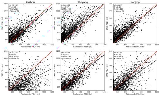
Figure 2.
Scatter plots of planetary boundary layer height (PBLH) derived from ERA5 and sounding datasets at (top) 08:00 LST and (bottom) 20:00 LST at the (a,d) Xuzhou, (b,e) Sheyang, and (c,f) Nanjing sites. R is the correlation coefficient, the star superscript indicates the value that is statistically significant (p < 0.01), RMSE is the root mean square error, the black solid line is the fitting line, and the red solid line is the reference line.
4. Results
4.1. Climatological Pattern of the PBLH
As a gross climatological overview, Figure 3 shows the spatial distribution of the mean PBLH at different times in Jiangsu. As shown in the figure, the PBLH was highest in the daytime (Figure 3b), ranging from 700 to 1200 m. At night (Figure 3d), the PBLH was lowest, ranging from 100 to 400 m. The morning (Figure 3a) and evening (Figure 3c) were in the transitional period between the daytime CBL and nighttime SBL, with PBLHs between 200 and 500 m. In the daytime, the PBLH was higher in the north and lower in the south. The highest PBLH was in the northwest, reaching 1200 m, and the lowest PBLH was in Hongze Lake in the western part and Tai Lake in the southern part of Jiangsu, at approximately 700 m. The PBLH in the eastern coastal areas was generally lower than that in the inland areas. At night, morning, and evening, the PBLH was lower in the north and higher in the south. The lowest PBLH was in the northwest, and the highest PBLH was in the two lakes (Hongze Lake in the west and Tai Lake in the south) and the eastern coastal area, with the highest PBLH reaching approximately 500 m.
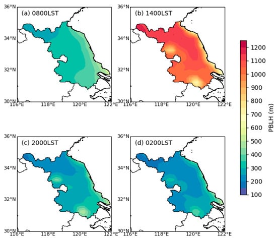
Figure 3.
Spatial distribution of the average PBLH over Jiangsu, China, from 1979 to 2019: (a) 08:00 LST, (b) 14:00 LST, (c) 20:00 LST, and (d) 02:00 LST.
4.2. Seasonal Variation
Figure 4 shows the seasonal distribution of the PBLH at different times in Jiangsu. As shown in the figure, in the daytime (14:00 LST), the PBLH ranged from 200 m to 2000 m, with a median of approximately 1000 m. In spring, the PBLH could reach more than 2000 m. The PBLH was usually highest in spring, followed by fall and summer, and lowest in winter. At night (02:00 LST), the PBLH was below 600 m, and the median was approximately 200 m. At night, morning (08:00, LST), and evening (20:00, LST), the PBLH generally followed a seasonal variation, that is, summer > spring > fall > winter, and the seasonal variation was more obvious in the morning.
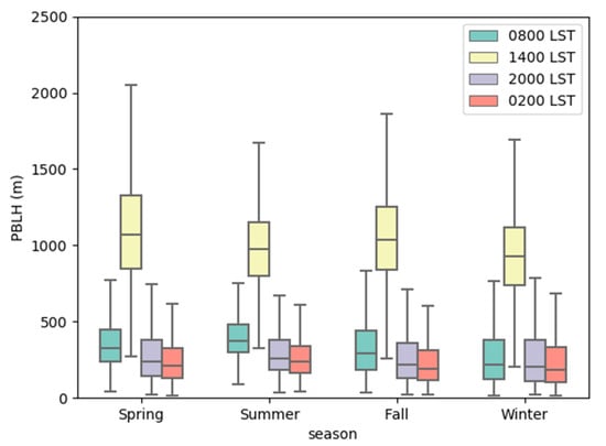
Figure 4.
Box-and-whisker plot of ERA5 PBLH during each season at 08:00, 14:00, 20:00, and 02:00 LST during the period from 1979 to 2019 over Jiangsu, China.
Figure 5 shows the spatial distribution of the seasonal mean PBLH at different times, revealing the spatial variation characteristics not shown in Figure 4. Figure 5a1–a4 shows that at 08:00 (LST, the same below), the seasonal variation in the PBLH in inland areas of Jiangsu was higher in spring and summer than in fall and winter. The average PBLH was approximately 300–500 m in spring and summer and 200–400 m in fall and winter. However, the seasonal variation in the PBLH in coastal areas was obviously opposite to that in inland areas, showing that the PBLH in autumn and winter was higher than that in spring and summer, and the average PBLH in autumn and winter was approximately 400–700 m. This may be because the PBLH in coastal areas is affected by the ocean and has the characteristics of the height of the marine atmospheric boundary layer that is lower in spring and summer and higher in autumn and winter due to the lower tropospheric stability [44,45]. The PBLH showed obvious southeast—northwest gradient changes over the four seasons. The PBLH was the highest in the southeast, reaching over 400 m in summer, the lowest in the northwest, and only approximately 200 m in winter. This may be because the southeast receives stronger solar radiation and the surface temperature is higher [26].

Figure 5.
Spatial distributions of the seasonal mean PBLH at 08:00 LST (a1–a4), 14:00 LST (b1–b4), 20:00 LST (c1–c4), and 02:00 LST (d1–d4) over Jiangsu, China.
At 14:00 (Figure 5b1–b4), the seasonal variation in the PBLH in inland areas of Jiangsu was ranked as spring > fall > summer > winter. The average PBLH in spring was approximately 1000–1400 m, and that in winter was approximately 900–1100 m. Affected by the ocean, the PBLH in coastal areas was still higher in fall and winter than in spring and summer. The spatial distribution of the PBLH in spring and summer was opposite to that at 08:00; that is, the PBLH in the northwest was higher than that in the southeast. In fall and winter, the highest PBLH appeared in central Jiangsu. Guo et al. [26] pointed out that the PBLH is higher in dry areas during the daytime. Compared with the southeastern part, the northwestern part of Jiangsu is drier, which means that in addition to solar radiation, humidity and other factors play an important role in controlling the spatial distribution of the PBLH during the daytime. At the same time, it can be noted that the PBLH at the two lakes was relatively low in all four seasons, especially in winter, when the average PBLH was below 700 m. This is because the high specific heat capacity of water causes the lake to warm up slowly and heat the atmosphere weakly, which then leads to the low PBLH.
At 20:00 (Figure 5c1–c4) and 02:00 (Figure 5d1–d4), the seasonal and spatial variables of the PBLH were generally similar to those at 08:00. However, since the SBL began to appear at night, the PBLH decreased, the average PBLH was approximately 100–500 m, and the seasonal variation was less obvious.
4.3. Diurnal Variation
The diurnal variation of the PBLH is also very important. Figure 6 shows the diurnal cycle of the PBLH in the four seasons in Jiangsu. As shown in the figure, in all seasons, the PBLH had obvious diurnal variation characteristics, and the difference between different seasons was small. The diurnal cycle of the PBLH was as follows: at night, the ground released longwave radiation, the surface cooled down, the near-surface layer was relatively stable, the PBLH decreased slowly, reaching the lowest point at 06:00 (LST), and the PBLH was approximately 200 m; after sunrise, the solar radiation increased and heated the ground, the CBL began to develop, and the PBLH gradually increased; in the afternoon, the PBLH reached its maximum, at approximately 900–1200 m; then, with the decrease in solar radiation, the turbulence intensity in CBL gradually attenuated, and the PBLH decreased rapidly; after sunset, the SBL began to form, and the PBLH remained low at night, approximately 200–300 m. At the same time, the decrease in the PBLH in the afternoon was more rapid than the increase in the PBLH in the morning, which is consistent with the findings of Liu and Liang. At night, the seasonal variation in the PBLH was very small, and the PBLH in summer was slightly higher than that in other seasons, which is consistent with the results of Gu et al. [45] In the daytime, especially in the afternoon (12:00–17:00 LST), the PBLH showed obvious seasonal variation, but the PBLH during summer was not the highest. In the afternoon, the PBLH was the highest in spring, followed by the PBLH in fall and summer, and the lowest was in winter, indicating that the PBLH in the daytime is related to other influencing factors besides solar radiation, which is analyzed in Section 4.4.
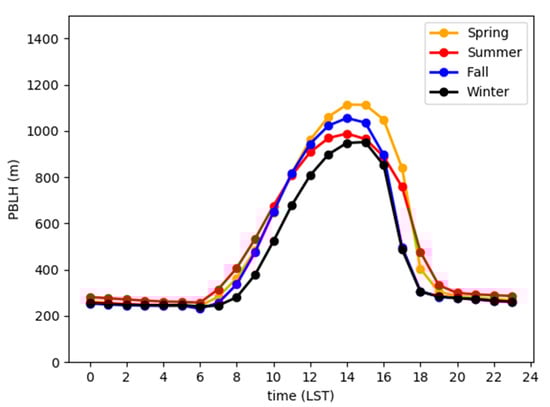
Figure 6.
Seasonal diurnal cycles of the mean PBLH throughout Jiangsu, China. The orange, red, blue, and black lines indicate spring, summer, fall, and winter, respectively.
Figure 7a–d shows the diurnal variation amplitude of the PBLH in Jiangsu, calculated by the daily maximum minus the minimum. As shown in the figure, the diurnal variation amplitude of the PBLH has obvious spatiotemporal characteristics. The amplitude in spring was the largest and decreased gradually from north to south. In spring, the strongest diurnal variation was in the northern area of Jiangsu, and the average diurnal variation amplitude was more than 1300 m. The diurnal variation was the weakest in the southern and coastal areas of Jiangsu, with an average amplitude below 700 m. The diurnal variation amplitude of fall and summer was lower than that of spring. The largest amplitude in fall was in central Jiangsu. The spatial distribution of the diurnal variation amplitude in summer was similar to that in spring, but the intensity was much weaker than that in spring. The diurnal variation amplitude of winter was the smallest. It is worth noting that the diurnal variation amplitude of the PBLH in coastal areas was smaller than that in inland areas, especially in spring and summer. At the same time, the diurnal variation amplitude of the PBLH in Hongze Lake and Tai Lake was also lower. This is because the high specific heat capacity of water leads to smaller diurnal variations in water temperature, which in turn leads to smaller diurnal variations in the PBLH [46]. Figure 7e–h shows the time when the daily PBLH reached its peak. As shown in the figure, in most areas, the PBLH reached its peak at 15:00 (LST) in spring and winter and at 14:00 (LST) in summer and fall. This difference corresponds to the time of sunrise. After sunrise, the ground heats up, which is the determining factor in the development of the PBL [24,47]. In spring and winter, the ground heating usually reaches its maximum at 15:00; thus, the PBLH usually reaches the peak at 15:00. While in summer and fall, due to earlier sunrises, the ground accumulates enough heat to reach the maximum earlier; therefore, the PBLH reaches the peak earlier. Furthermore, the time when the PBLH reached its peak in the eastern area of Jiangsu was usually earlier than that in the western area, which was also because the time of sunrise in the eastern area was earlier.
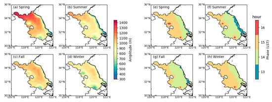
Figure 7.
(a–d) Amplitude and (e–h) phase of the diurnal cycle of the PBLH over Jiangsu, China, for each season. Amplitudes are mean values of daily maximum minus daily minimum, and phases are the hour of maximum PBLH.
4.4. Factors that Affect PBLH Diurnal Variation
In addition to solar radiation, the PBLH also has a significant relationship with meteorological factors [20]. According to a study by Gu et al. [45], the diurnal cycle of the PBLH is significantly positively correlated with the near-surface temperature and negatively correlated with the relative humidity. Zhang et al. [25] noted that higher surface temperature and lower relative humidity lead to higher sensible heat flux and lower latent heat flux, resulting in deeper convection and a higher PBLH. To further understand the influence of meteorological factors on the diurnal cycle of the PBLH in Jiangsu and analyze the reason for the seasonal variation in the diurnal cycle, we study the diurnal cycles of several meteorological factors in the four seasons and calculate the correlations between them and the PBLH. The selected meteorological factors include 2 m temperature (T2m), 10 m wind speed (WS), near-surface relative humidity (RH), and lower tropospheric stability (LTS). LTS is defined as the potential temperature difference between 700 hPa and the surface, which can represent the thermodynamic state of the low troposphere. A larger LTS usually reflects a more stable low troposphere [48,49].
Figure 8 shows the diurnal cycles of meteorological factors in the four seasons. Comparing the diurnal cycle of the PBLH (Figure 6), we find that the diurnal cycles of T2m and WS have a positive relationship with the diurnal cycle of the PBLH. A higher T2m and stronger WS correspond to a higher PBLH, indicating that stronger surface heating and surface forcing contribute to the development of the PBL. On the other hand, the diurnal cycles of RH and LTS have obvious inverse relationships with the diurnal cycle of the PBLH. A lower RH and lower LTS correspond to a higher PBLH because the lower the RH is, the lower the latent heat flux, the more sensible the heat flux is, and the stronger the development of the PBL is. Moreover, the lower the LTS is, the more conducive it is to convective activity and the easier it is to develop the PBL. Figure 6 also shows that at night, the PBLH in summer was slightly higher than that in other seasons. This may have been due to the higher T2m (Figure 8a) and lower LTS (Figure 8d) in summer. However, during the daytime, the highest PBLH occurred in spring, not in summer. Figure 8b,c shows that in the daytime, the WS of spring was highest and the RH was lowest, while in summer, the WS was lower, and the RH was higher. Therefore, it can be concluded that the seasonal variation in daytime PBLH is more related to WS and RH. The PBLH was the highest in spring, which may have been due to the high WS in spring [50,51]. High WS enhances low-layer wind shear and upward forcing, thus enhancing turbulence and increasing the PBLH. The lower PBLH in summer may be because Jiangsu is in the plum rain season with high RH and more precipitation [52]. Water vapor absorbs more heat, which reduces the heating efficiency of the surface to the air, thus inhibiting the development of the PBL.
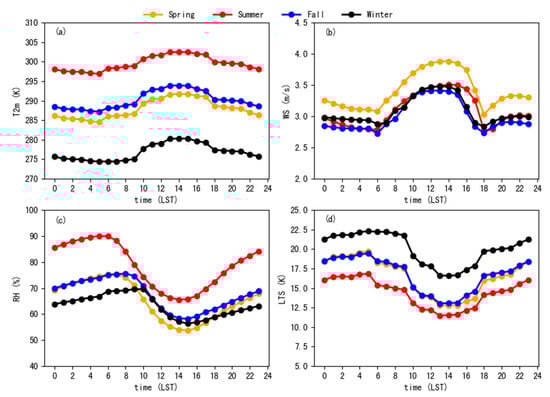
Figure 8.
Diurnal cycle of the average (a) 2 m temperature (T2m), (b) 10 m wind speed (WS), (c) relative humidity (RH), and (d) lower tropospheric stability (LTS) over Jiangsu, China.
We calculate the correlation coefficients between the PBLH and meteorological factors based on the diurnal cycles in the four seasons (Table 1), with bold data indicating significant correlations at the 95% or higher confidence level. The results show that the diurnal cycle of the PBLH is significantly correlated with the diurnal cycle of meteorological factors in the four seasons. Specifically, the PBLH is significantly positively correlated with the T2m and WS and significantly negatively correlated with the RH and LTS. This is consistent with the research results of Gu et al. [45]. These correlations indicate that on the daily scale, higher T2m and WS and lower RH and LTS will correspond to higher PBLH.

Table 1.
Correlation coefficients between the PBLH and meteorological variables (2 m temperature (T2m), 10 m wind speed (WS), relative humidity (RH), and lower tropospheric stability (LTS)) based on the diurnal cycle in the four seasons over Jiangsu, China. Bold figures are significant at the 95% confidence level or greater.
4.5. Long-Term Trend of PBLH over Jiangsu and Causes
In addition to the climatic characteristics and influencing factors of the PBLH, the long-term variation trend of the PBLH is another issue that needs attention. We calculated the variation trend of the annual mean PBLH from 1979 to 2019 in Jiangsu. The results show that the daytime PBLH had a significant increasing trend (Figure 9), while the PBLH at night had no significant variation trend (not shown), which is consistent with the results of Zhang et al. [31] and Gu et al. [45]. Figure 9a shows the time series of the daytime (14:00 LST) annual mean PBLH in Jiangsu. As shown in the figure, the daytime PBLH had an increasing trend, especially since the 1990s, when the PBLH had obviously increased. Figure 9b shows the trend of the PBLH in Jiangsu. The results show that the PBLH in most areas of Jiangsu had a significant growth trend, and the fastest growing areas were in the central and southern areas of Jiangsu, with the highest trend reaching 3 m·yr−1.
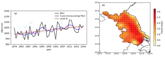
Figure 9.
(a) Time series of annual mean BLH (black line) and 5-year moving average BLH (blue line) throughout Jiangsu, China, at 14:00 LST for the 1979–2019 period. The red line denotes the linear fitting trend. (b) Spatial distribution of the trend of annual mean BLH over Jiangsu, China, at 14:00 LST during 1979–2019. Black dots indicate trends that are statistically significant (p < 0.05).
To explore the reason for the increase in the daytime PBLH, we analyze the variation trend of the impact factors from 1979 to 2019. The results show that daytime T2m, RH, and LTS had significant variation trends (Figure 10 and Figure 11), but WS had no significant variation trend (not shown). Figure 10 shows the time series of the daytime (14:00 LST) annual mean T2m, RH, and LTS and the correlation coefficients with the annual mean PBLH. The annual mean PBLH has a significantly positive correlation with T2m, with a correlation coefficient of 0.56 (Figure 10a), and a significantly negative correlation with RH and LTS, with correlation coefficients of −0.9 and −0.82, respectively (Figure 10b,c). At the same time, we also find that in the past 41 years, T2m had obviously increased, and RH and LTS had obviously decreased, especially since the 1990s. This is consistent with the findings of Xia et al. [53] and Chen et al. [54]. Therefore, we can calculate the variation trend of meteorological factors in Jiangsu (Figure 11). The results show that T2m had a significantly increasing trend, and RH and LTS had significantly decreasing trends. At the same time, we find that the spatial distribution of the variation trend of meteorological factors was similar to that of the PBLH; that is, the T2m in the southern area increased faster than that in the northern area, and the RH and LTS also decreased faster, which may be the reason for the faster growth of the PBLH in the south.
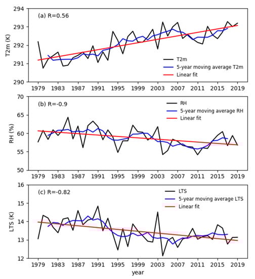
Figure 10.
Same as Figure 9a, but for the time series of (a) T2m, (b) RH, and (c) LTS. R is the correlation coefficient between the annual mean PBLH and meteorological variables.
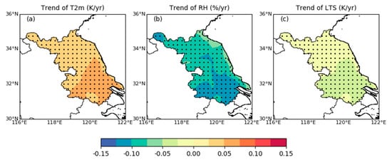
Figure 11.
Same as Figure 9b, but for the spatial distribution of the trend of (a) T2m, (b) RH, and (c) LTS.
Finally, we calculate the correlation coefficients between the annual mean PBLH and T2m and RH and LTS in Jiangsu (Figure 12). The results show that the annual mean PBLH has a significantly positive correlation with T2m and a significantly negative correlation with RH and LTS. Moreover, the areas with the strongest correlation correspond to the areas with the fastest-growing trend of the PBLH. Therefore, we can conclude that the increase in daytime PBLH may be due to the increase in T2m and the decrease in RH and LTS. This is consistent with the above results: higher T2m, lower RH, and lower LTS contribute to a higher PBLH.
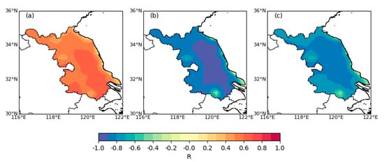
Figure 12.
Spatial distribution of correlation coefficients (R) between annual mean BLH and (a) T2m, (b) RH, and (c) LTS during 1979–2019.
5. Conclusions and Discussion
Based on the hourly reanalysis data from ERA5 from 1979 to 2019, the climatology of the PBLH in Jiangsu, China, is studied in this paper.
The PBLH based on ERA5 is first verified by radiosonde data, and the results show that the PBLH based on ERA5 fits very well with the PBLH diagnosed by radiosonde data, with correlation coefficients exceeding 0.7 at all three stations. This shows that it is valid to use the PBLH based on ERA5 data in the Jiangsu region.
In Jiangsu, the daytime PBLH was highest, and the average PBLH was approximately 700–1200 m, which was higher in the north and lower in the south. At night, the PBLH was lowest, and the average PBLH was between 100 and 400 m, being lower in the north and higher in the south. The PBLH exhibited complex spatiotemporal variation. In the daytime, the PBLH in inland areas was highest in spring, followed by fall and summer, and lowest in winter. A higher wind speed in spring produces stronger ground forcing, which increases the PBLH. Higher relative humidity in summer increases the latent heat flux and decreases the sensible heat flux, leading to a lower PBLH. At night, the seasonal variation in the PBLH was less obvious. Affected by the ocean, the seasonal variation in the PBLH in coastal areas was opposite to that in inland areas, higher in fall and winter and lower in spring and summer.
The PBLH had an obvious diurnal cycle, usually reaching its peak at 14:00 (LST) or 15:00 (LST). The diurnal variation in the PBLH was largest in spring and smallest in winter. The diurnal cycle of the PBLH was significantly positively correlated with the near-surface temperature and wind speed and significantly negatively correlated with the near-surface relative humidity and lower tropospheric stability. Over these 41 years, the daytime PBLH had a significantly increasing trend in most areas. The increase in PBLH can be attributed to the increase in near-surface temperature and the decrease in near-surface relative humidity and lower tropospheric stability.
The results of this paper will deepen the understanding of the spatiotemporal distribution characteristics of the PBLH and its effecting factors in eastern China. But we also clearly recognized that there were still some uncertainties in this article. On the one hand, the lack of observations makes it difficult to confirm the accuracy of the temporal trend of the PBLH in the ERA5 dataset. Also, the differences between PBLH detection methods also lead to great uncertainties in the PBLH [55,56]. On the other hand, the impact of the PBLH on weather forecasting, climate, and air quality prediction was not specifically explored here. Previous studies have revealed that the PBLH was one of the most important physical parameters in the numerical model and atmospheric environment assessment, which reflects the physical processes, such as turbulent mixing and convection development, in the boundary layer and affects the vertical distribution of heat, water vapor, aerosols, and other materials and energy [57,58]. In terms of weather forecasting and climate prediction, the results of this paper can be used to evaluate the simulation performance of different boundary layer parameterization schemes and optimize the schemes applicable to the Jiangsu region, which has a potential impact on improving the forecast skill in this region [59]. In terms of air quality assessment, some studies have confirmed that the PBLH is negatively correlated with the concentration of pollutants in the surface layer, and the relationship can be expressed as a power function under convective conditions [4,60]. The interaction between aerosols and the boundary layer is mainly characterized by how the increase in aerosol content will weaken the solar radiation reaching the surface [61,62,63]. Through the aerosol boundary layer feedback mechanism, the inversion of the boundary layer is strengthened, the turbulent diffusion is weakened, the height of the boundary layer is reduced, and water vapor and pollutants are further accumulated [64,65,66]. Moreover, the PBLH can be associated with many interesting studies in the local context, including, but not limited to, urban climatic conditions, urban heat islands/heat waves, air pollution, etc. [67,68,69,70]. In the near future, we will conduct more work on these specific applications, like analyzing the relationship and mechanism between air pollution and the PBLH in the Jiangsu region.
Author Contributions
Conceptualization, X.L.; methodology, X.L. and Y.D.; formal analysis, Y.D.; investigation, Y.D.; data curation, J.Y.; writing—original draft preparation, X.L. and Y.D.; writing—Review and editing, Y.Z. and Z.S. All authors have read and agreed to the published version of the manuscript.
Funding
This work is supported by the National Key R&D Program of China (2019YFC1408004), the National Natural Science Foundation of China (42276020, 42205064), and the Scientific research project of the China Three Gorges Corporation (Grant. Nos. 202103460).
Institutional Review Board Statement
The study does not require ethical approval, excluding this statement.
Informed Consent Statement
The study does not involve humans, excluding this statement.
Data Availability Statement
The ERA5 dataset used in the study is available from: https://cds.climate.copernicus.eu/cdsapp#!/home (accessed on 1 May 2023).
Acknowledgments
We thank the anonymous reviewers for their comments, which improved the paper.
Conflicts of Interest
The authors declare no conflict of interest.
References
- Stull, R.B. An Introduction to Boundary Layer Meteorology; Kluwer Academic: Dordrecht, The Netherlands, 1988; p. 666. [Google Scholar]
- Bakas, N.A.; Fotiadi, A.; Kariofillidi, S. Climatology of the Boundary Layer Height and of the Wind Field over Greece. Atmosphere 2020, 11, 910. [Google Scholar] [CrossRef]
- Davies, F.; Middleton, D.R.; Bozier, K.E. Urban air pollution modelling and measurements of boundary layer height. Atmos. Environ. 2007, 41, 4040–4049. [Google Scholar] [CrossRef]
- Quan, J.; Gao, Y.; Zhang, Q.; Tie, X.; Cao, J.; Han, S.; Meng, J.; Chen, P.; Zhao, D. Evolution of planetary boundary layer under different weather conditions, and its impact on aerosol concentrations. Particuology 2013, 11, 34–40. [Google Scholar] [CrossRef]
- Yang, T.; Wang, Z.; Zhang, W.; Gbaguidi, A.; Sugimoto, N.; Wang, X.; Matsui, I.; Sun, Y. Technical note: Boundary layer height determination from lidar for improving air pollution episode modeling: Development of new algorithm and evaluation. Atmos. Chem. Phys. 2017, 17, 6215–6225. [Google Scholar] [CrossRef]
- Dang, R.; Qiu, X.; Yang, Y.; Zhang, S. Observation system simulation experiments (OSSEs) for assimilation of the planetary boundary-layer height (PBLH) using the EnSRF technique. Q. J. R. Meteorol. Soc. 2022, 148, 1184–1207. [Google Scholar] [CrossRef]
- Mak, H.W.L. Improved Remote Sensing Algorithms and Data Assimilation Approaches in Solving Environmental Retrieval Problems. Ph.D. Thesis, Hong Kong University of Science and Technology, Hong Kong, China, 2019. [Google Scholar]
- Yue, M.; Wang, M.; Guo, J.; Zhang, H.; Dong, X.; Liu, Y. Long-Term Trend Comparison of Planetary Boundary Layer Height in Observations and CMIP6 Models over China. J. Clim. 2021, 34, 8237–8256. [Google Scholar] [CrossRef]
- Seidel, D.J.; Ao, C.O.; Li, K. Estimating climatological planetary boundary layer heights from radiosonde observations: Comparison of methods and uncertainty analysis. J. Geophys. Res. 2010, 115, D16113. [Google Scholar] [CrossRef]
- Hennemuth, B.; Lammert, A. Determination of the Atmospheric Boundary Layer Height from Radiosonde and Lidar Backscatter. Bound.-Layer Meteorol. 2006, 120, 181–200. [Google Scholar] [CrossRef]
- Tucker, S.C.; Senff, C.J.; Weickmann, A.M.; Brewer, W.A.; Banta, R.M.; Sandberg, S.P.; Law, D.C.; Hardesty, R.M. Doppler Lidar Estimation of Mixing Height Using Turbulence, Shear, and Aerosol Profiles. J. Atmos. Ocean. Technol. 2009, 26, 673–688. [Google Scholar] [CrossRef]
- Angevine, W.M.; White, A.B.; Avery, S.K. Boundary-layer depth and entrainment zone characterization with a boundary-layer profiler. Bound.-Layer Meteorol. 1994, 68, 375–385. [Google Scholar] [CrossRef]
- Bianco, L.; Wilczak, J.M. Convective Boundary Layer Depth: Improved Measurement by Doppler Radar Wind Profiler Using Fuzzy Logic Methods. J. Atmos. Ocean. Technol. 2002, 19, 1745–1758. [Google Scholar] [CrossRef]
- Eresmaa, N.; Karppinen, A.; Joffre, S.M.; Räsänen, J.; Talvitie, H. Mixing height determination by ceilometer. Atmos. Chem. Phys. Discuss. 2006, 6, 1485–1493. [Google Scholar] [CrossRef]
- Kamp, D.; Mckendry, I. Diurnal and Seasonal Trends in Convective Mixed-Layer Heights Estimated from Two Years of Continuous Ceilometer Observations in Vancouver, BC. Bound.-Layer Meteorol. 2010, 137, 459–475. [Google Scholar] [CrossRef]
- Ratnam, M.V.; Basha, S.G. A robust method to determine global distribution of atmospheric boundary layer top from COSMIC GPS RO measurements. Atmos. Sci. Lett. 2010, 11, 216–222. [Google Scholar] [CrossRef]
- Ao, C.O.; Waliser, D.E.; Chan, S.K.; Li, J.L.; Tian, B.; Xie, F.; Mannucci, A.J. Planetary boundary layer heights from GPS radio occultation refractivity and humidity profiles. J. Geophys. Res. Atmos. 2012, 117, D16117. [Google Scholar] [CrossRef]
- Su, T.; Li, J.; Li, C.; Xiang, P.; Lau, A.K.-H.; Guo, J.; Yang, D.; Miao, Y. An intercomparison of long-term planetary boundary layer heights retrieved from CALIPSO, ground-based lidar, and radiosonde measurements over Hong Kong. J. Geophys. Res. Atmos. 2017, 122, 3929–3943. [Google Scholar] [CrossRef]
- Zhang, W.; Guo, J.; Miao, Y.; Liu, H.; Zhang, Y.; Li, Z.; Zhai, P. Planetary boundary layer height from CALIOP compared to radiosonde over China. Atmos. Chem. Phys. 2016, 16, 9951–9963. [Google Scholar] [CrossRef]
- Seidel, D.J.; Zhang, Y.; Beljaars, A.; Golaz, J.C.; Jacobson, A.R.; Medeiros, B. Climatology of the planetary boundary layer over the continental United States and Europe. J. Geophys. Res. Atmos. 2012, 117, D17106. [Google Scholar] [CrossRef]
- von Engeln, A.; Teixeira, J. A Planetary Boundary Layer Height Climatology Derived from ECMWF Reanalysis Data. J. Clim. 2013, 26, 6575–6590. [Google Scholar] [CrossRef]
- Si, Y.; Li, S.; Chen, L.; Yu, C.; Wang, Z.; Wang, Y.; Wang, H. Validation and Spatiotemporal Distribution of GEOS-5–Based Planetary Boundary Layer Height and Relative Humidity in China. Adv. Atmos. Sci. 2018, 35, 479–492. [Google Scholar] [CrossRef]
- Holzworth, G.C. Estimates of Mean Maximum Mixing Depths in the Contiguous United States. Mon. Weather Rev. 1964, 92, 235–242. [Google Scholar] [CrossRef]
- Liang, X.-Z.; Liu, S. Observed Diurnal Cycle Climatology of Planetary Boundary Layer Height. J. Clim. 2010, 23, 5790–5809. [Google Scholar]
- Zhang, Y.; Zhang, S.; Huang, C.; Huang, K.; Gong, Y.; Gan, Q. Diurnal variations of the planetary boundary layer height estimated from intensive radiosonde observations over Yichang, China. Sci. China Technol. Sci. 2014, 57, 2172–2176. [Google Scholar] [CrossRef]
- Guo, J.; Miao, Y.; Zhang, Y.; Liu, H.; Li, Z.; Zhang, W.; He, J.; Lou, M.; Yan, Y.; Bian, L.; et al. The climatology of planetary boundary layer height in China derived from radiosonde and reanalysis data. Atmos. Chem. Phys. 2016, 16, 13309–13319. [Google Scholar] [CrossRef]
- Guo, J.; Li, Y.; Cohen, J.B.; Li, J.; Chen, D.; Xu, H.; Liu, L.; Yin, J.; Hu, K.; Zhai, P. Shift in the Temporal Trend of Boundary Layer Height in China Using Long-Term (1979–2016) Radiosonde Data. Geophys. Res. Lett. 2019, 46, 6080–6089. [Google Scholar] [CrossRef]
- Zhao, C.; Li, Y.; Liu, Y.; Zhou, G. The variation characteristics of planetary boundary layer height in Northwest China: Based on radiosonde and ERA-Interim reanalysis data. Plateau Meteorol. 2019, 38, 1181–1193. [Google Scholar]
- Zhao, Y.; Mao, W.; Zhang, K.; Ma, Y.; Li, H.; Zhang, W. Climatic Variations in the Boundary Layer Height of Arid and Semiarid Areas in East Asia and North Africa. J. Meteorol. Soc. Japan. Ser. II 2017, 95, 181–197. [Google Scholar] [CrossRef]
- Allabakash, S.; Lim, S. Climatology of Planetary Boundary Layer Height-Controlling Meteorological Parameters over the Korean Peninsula. Remote Sens. 2020, 12, 2571. [Google Scholar] [CrossRef]
- Zhang, Y.; Seidel, D.J.; Zhang, S. Trends in Planetary Boundary Layer Height over Europe. J. Clim. 2013, 26, 10071–10076. [Google Scholar] [CrossRef]
- Li, J.; Chu, Y.; Li, X.; Dong, Y. Long-term trends of global maximum atmospheric mixed layer heights derived from radiosonde measurements. Environ. Res. Lett. 2020, 15, 034054. [Google Scholar] [CrossRef]
- Yang, D.; Li, C.; Lau, K.H.; Li, Y. Long-term measurement of daytime atmospheric mixing layer height over Hong Kong. J. Geophys. Res. Atmos. 2013, 118, 2422–2433. [Google Scholar] [CrossRef]
- Slingo, J.M. The Development and Verification of A Cloud Prediction Scheme for the Ecmwf Model. Q. J. R. Meteorol. Soc. 1987, 113, 899–927. [Google Scholar] [CrossRef]
- Basha, G.; Ratnam, M.V. Identification of atmospheric boundary layer height over a tropical station using high-resolution radiosonde refractivity profiles: Comparison with GPS radio occultation measurements. J. Geophys. Res. 2009, 114, D16101. [Google Scholar] [CrossRef]
- Tang, G.; Zhang, J.; Zhu, X.; Song, T.; Münkel, C.; Hu, B.; Schäfer, K.; Liu, Z.; Zhang, J.; Wang, L.; et al. Mixing layer height and its implications for air pollution over Beijing, China. Atmos. Chem. Phys. 2016, 16, 2459–2475. [Google Scholar] [CrossRef]
- Davis, E.V.; Rajeev, K.; Mishra, M.K. Effect of Clouds on the Diurnal Evolution of the Atmospheric Boundary-Layer Height Over a Tropical Coastal Station. Bound.-Layer Meteorol. 2020, 175, 135–152. [Google Scholar] [CrossRef]
- Chan, K.M.; Wood, R. The seasonal cycle of planetary boundary layer depth determined using COSMIC radio occultation data. J. Geophys. Res. Atmos. 2013, 118, 412–422, 434. [Google Scholar] [CrossRef]
- Sicard, M.; Pérez, C.; Rocadenbosch, F.; Baldasano, J.M.; García-Vizcaino, D. Mixed-Layer Depth Determination in the Barcelona Coastal Area From Regular Lidar Measurements: Methods, Results and Limitations. Bound.-Layer Meteorol. 2006, 119, 135–157. [Google Scholar] [CrossRef]
- Sen, K.P. Estimates of the Regression Coefficient Based on Kendall’s Tau. Publ. Am. Stat. Assoc. 1968, 63, 1379–1389. [Google Scholar] [CrossRef]
- Mann, H.B. Nonparametric test against trend. Econometrica 1945, 13, 245–259. [Google Scholar] [CrossRef]
- Kendall, M.G. Rank Correlation Methods. Br. J. Psychol. 1990, 25, 86–91. [Google Scholar] [CrossRef]
- Meng, X.; Guo, J.; Han, Y. Preliminarily assessment of ERA5 reanalysis data. J. Mar. Meteorol. 2018, 38, 91–99. [Google Scholar]
- Nozaki, K.Y. Mixing Depth Model Using Hourly Surface Observations; Report 7053; USAF Environmental Technical Applications Center: Patrick Air Force Base, FL, USA, 1973. [Google Scholar]
- Gu, J.; Zhang, Y.; Yang, N.; Wang, R. Diurnal variability of the planetary boundary layer height estimated from radiosonde data. Earth Planet. Phys. 2020, 4, 479–492. [Google Scholar] [CrossRef]
- Johnson, R.H.; Ciesielski, P.E.; Cotturone, J.A. Multiscale Variability of the Atmospheric Mixed Layer over the Western Pacific Warm Pool. J. Atmos. Sci. 2001, 58, 2729–2750. [Google Scholar] [CrossRef]
- Jie, J.; Youfei, Z.; Jianjun, L.; Jinjin, F. Observational research on planetary boundary layer by lidar over Nanjing city. Environ. Sci. Technol. 2014, 37, 22–27. [Google Scholar]
- Guo, J.; Deng, M.; Lee, S.S.; Wang, F.; Li, Z.; Zhai, P.; Liu, H.; Lv, W.; Yao, W.; Li, X. Delaying precipitation and lightning by air pollution over the Pearl River Delta. Part I: Observational analyses. J. Geophys. Res. Atmos. 2016, 121, 6472–6488. [Google Scholar] [CrossRef]
- Guo, J.; Su, T.; Li, Z.; Miao, Y.; Li, J.; Liu, H.; Cribb, M.; Zhai, P. Declining frequency of summertime local-scale precipitation over eastern China from 1970 to 2010 and its potential link to aerosols. Geophys. Res. Lett. 2017, 44, 5700–5708. [Google Scholar] [CrossRef]
- Zhao, X.; Zhang, X.; Xu, X.; Jing, X.; Meng, W.; Pu, W. Seasonal and diurnal variations of ambient PM2.5 concentration in urban and rural environments in Beijing. Atmos. Environ. 2009, 43, 2893–2900. [Google Scholar] [CrossRef]
- Hua, G.; Ming, X.; Qi, H. Changes in near-surface wind speed in China: 1969–2005. Int. J. Climatol. 2011, 31, 349–358. [Google Scholar]
- Mao, W.; Wang, Q.; Ma, H.; Shen, G. Temporal and Spatial Variation Characteristics of Meiyu in Jianghuai. Trans. Atmos. Sci. 2008, 31, 116–122. [Google Scholar]
- Xia, L.; Zhang, Q.; Sun, N.; Wang, S. Climate change characteristics in Jiangsu Province, 1960–2012. J. Glaciol. Geocryol. 2015, 37, 1480–1489. [Google Scholar]
- Chen, J.; Zhong, S. Analysis of characteristics of relative humidity changes in Nanjing from 1961 to 2010. Energy Res. Util. 2018, 4, 45–49. [Google Scholar]
- Zhang, Y.; Li, S. Climatological characteristics of planetary boundary layer height over Japan. Int. J. Climatol. 2019, 39, 4015–4028. [Google Scholar] [CrossRef]
- Slättberg, N.; Lai, H.W.; Chen, X.; Ma, Y.; Chen, D. Spatial and temporal patterns of planetary boundary layer height during 1979–2018 over the Tibetan Plateau using ERA5. Int. J. Climatol. 2021, 42, 3360–3377. [Google Scholar] [CrossRef]
- Seibert, P.; Beyrich, F.; Gryning, S.E.; Joffre, S.; Rasmussen, A.; Tercier, P. Review and intercomparison of operational methods for the determination of the mixing height. Atmos. Environ. 2000, 34, 1001–1027. [Google Scholar] [CrossRef]
- Zhang, Q.; Zhang, J.; Qiao, J.; Wang, S. Relationship of atmospheric boundary layer depth with thermodynamic processes at the land surface in arid regions of China. Sci. China Earth Sci. 2011, 54, 1586–1594. [Google Scholar] [CrossRef]
- Hong, S.Y.; Pan, H.L. Nonlocal boundary layer vertical diffusion in a medium-range forecast model. Mon. Weather Rev. 1996, 124, 2322–2339. [Google Scholar] [CrossRef]
- Li, Q.; Wu, B.; Liu, J.; Zhang, H.; Song, Y. Characteristics of the atmospheric boundary layer and its relation with PM 2.5 during haze episodes in winter in the North China Plain. Atmos. Environ. 2020, 223, 117265. [Google Scholar] [CrossRef]
- Ma, Y.; Ye, J.; Xin, J.; Zhang, W.; Vilà-Guerau de Arellano, J.; Wang, S.; Zhao, D.; Dai, L.; Ma, Y.; Wu, X.; et al. The Stove, Dome, and Umbrella Effects of Atmospheric Aerosol on the Development of the Planetary Boundary Layer in Hazy Regions. Geophys. Res. Lett. 2020, 47, e2020GL087373. [Google Scholar] [CrossRef]
- Ding, A.J.; Huang, X.; Nie, W.; Sun, J.N.; Kerminen, V.M.; Petäjä, T. Enhanced haze pollution by black carbon in megacities in China. Geophys. Res. Lett. 2016, 43, 2873–2879. [Google Scholar] [CrossRef]
- Ma, Y.; Xin, J.; Wang, Z.; Tian, Y.; Wu, L.; Tang, G.; Zhang, W.; Vilà-Guerau de Arellano, J.; Zhao, D.; Jia, D.; et al. How do aerosols above the residual layer affect the planetary boundary layer height? Sci. Total Environ. 2022, 814, 151953. [Google Scholar] [CrossRef]
- Ding, A.J.; Fu, C.B.; Yang, X.Q.; Sun, J.N.; Petäjä, T.; Kerminen, V.M.; Wang, T.; Xie, Y.; Herrmann, E.; Zheng, L.F. Intense atmospheric pollution modifies weather: A case of mixed biomass burning with fossil fuel combustion pollution in eastern China. Atmos. Chem. Phys. 2013, 13, 10545–10554. [Google Scholar] [CrossRef]
- Li, Z. Aerosol and boundary-layer interactions and impact on air quality. Natl. Sci. Rev. 2017, 4, 810–833. [Google Scholar] [CrossRef]
- Zou, J.; Sun, J.; Ding, A.; Wang, M.; Guo, W.; Fu, C. Observation-based estimation of aerosol-induced reduction of planetary boundary layer height. Adv. Atmos. Sci. 2017, 34, 1057–1068. [Google Scholar] [CrossRef]
- Wu, Y.; Zhao, K.; Huang, J.; Arend, M.; Moshary, F. Observation of heat wave effects on the urban air quality and PBL in New York City area. Atmos. Environ. 2019, 218, 117024. [Google Scholar] [CrossRef]
- He, Y.; Ren, C.; Mak, H.W.L.; Lin, C.; Ng, E. Investigations of high-density urban boundary layer under summer prevailing wind conditions with Doppler LiDAR: A case study in Hong Kong. Urban Clim. 2021, 38, 100884. [Google Scholar] [CrossRef]
- Yin, J.; Gao, C.Y.; Hong, J.; Gao, Z.; Li, Y.; Li, X.; Fan, S.; Zhu, B. Surface Meteorological Conditions and Boundary Layer Height Variations During an Air Pollution Episode in Nanjing, China. J. Geophys. Res. Atmos. 2019, 124, 3350–3364. [Google Scholar] [CrossRef]
- Qu, Y.; Han, Y.; Wu, Y.; Gao, P.; Wang, T. Study of PBLH and Its Correlation with Particulate Matter from One-Year Observation over Nanjing, Southeast China. Remote Sens. 2017, 9, 668. [Google Scholar] [CrossRef]
Disclaimer/Publisher’s Note: The statements, opinions and data contained in all publications are solely those of the individual author(s) and contributor(s) and not of MDPI and/or the editor(s). MDPI and/or the editor(s) disclaim responsibility for any injury to people or property resulting from any ideas, methods, instructions or products referred to in the content. |
© 2023 by the authors. Licensee MDPI, Basel, Switzerland. This article is an open access article distributed under the terms and conditions of the Creative Commons Attribution (CC BY) license (https://creativecommons.org/licenses/by/4.0/).