Article

Intriguing Aspects of Polar-to-Tropical Mesospheric Teleconnections during the 2018 SSW: A Meteor Radar Network Study

by
Sunkara Eswaraiah
1,2,*,
Kyong-Hwan Seo
1,3,*,
Kondapalli Niranjan Kumar
4,
Andrey V. Koval
5,
Madineni Venkat Ratnam
6,
Chalachew Kindie Mengist
1,
Gasti Venkata Chalapathi
7,
Huixin Liu
8,
Young-Sil Kwak
9,
Eugeny Merzlyakov
10,11,
Christoph Jacobi
12,
Yong-Ha Kim
13,
Sarangam Vijaya Bhaskara Rao
14 and
Nicholas J. Mitchell
15
1
Research Center for Climate Sciences, Pusan National University, Busan 46241, Republic of Korea
2
Centre for Atmospheric and Space Science, Mohan Babu University, Tirupati 517102, India
3
Department of Atmospheric Sciences, Pusan National University, Busan 46241, Republic of Korea
4
National Centre for Medium Range Weather Forecasting, Noida 201301, India
5
Atmospheric Physics Department, Saint Petersburg State University, 198504 Saint Petersburg, Russia
6
National Atmospheric Research Laboratory, Tirupati 517502, India
7
Department of Physics, Government Degree College, Anantapur 515001, India
8
Department of Earth and Planetary Sciences, Kyushu University, Fukuoka 819-0395, Japan
9
Space Science Division, Korea Astronomy and Space Science Institute, Daejeon 34055, Republic of Korea
10
Institute for Experimental Meteorology, Science and Production Association “Typhoon”, 249030 Obninsk, Russia
11
Radiophysics Department, Kazan (Volga Region) Federal University, 420008 Kazan, Russia
12
Institute for Meteorology, Leipzig University, 04103 Leipzig, Germany
13
Department of Astronomy and Space Science, Chungnam National University, Daejeon 34134, Republic of Korea
14
Department of Physics, Sri Venkateswara University, Tirupati 517502, India
15
Department of Electronic & Electrical Engineering, University of Bath, Bath BA2 7AY, UK
*
Authors to whom correspondence should be addressed.
Atmosphere 2023, 14(8), 1302; https://doi.org/10.3390/atmos14081302
Submission received: 26 June 2023 / Revised: 12 August 2023 / Accepted: 13 August 2023 / Published: 17 August 2023
(This article belongs to the Section Atmospheric Techniques, Instruments, and Modeling)

Abstract

:
Using a network of meteor radar observations, observational evidence of polar-to-tropical mesospheric coupling during the 2018 major sudden stratosphere warming (SSW) event in the northern hemisphere is presented. In the tropical lower mesosphere, a maximum zonal wind reversal (−24 m/s) is noted and compared with that identified in the extra-tropical regions. Moreover, a time delay in the wind reversal between the tropical/polar stations and the mid-latitudes is detected. A wide spectrum of waves with periods of 2 to 16 days and 30–60 days were observed. The wind reversal in the mesosphere is due to the propagation of dominant intra-seasonal oscillations (ISOs) of 30–60 days and the presence and superposition of 8-day period planetary waves (PWs). The ISO phase propagation is observed from high to low latitudes (60° N to 20° N) in contrast to the 8-day PW phase propagation, indicating the change in the meridional propagation of winds during SSW, hence the change in the meridional circulation. The superposition of dominant ISOs and weak 8-day PWs could be responsible for the delay of the wind reversal in the tropical mesosphere. Therefore, this study has strong implications for understanding the reversed (polar to tropical) mesospheric meridional circulation by considering the ISOs during SSW.

1. Introduction

Sudden stratospheric warming (SSW) [1,2,3] is one of the most remarkable and extreme atmospheric phenomena that occur in the boreal winter, causing the polar vortex to distort and, at times, even break down [4]. In recent years, SSW events have attracted significant attention due to their role in changing the Earth’s middle and upper atmospheric structure and dynamics on a large scale in both hemispheres [5], thereby affecting the surface weather on a continental scale [6,7]. The mechanism of SSW is well documented [2]. However, significant ambiguities still exist in defining major and minor SSW events and their specific parameters [8]. SSW events occur approximately six times per decade in the northern hemisphere (NH) [3,9]. However, due to the weak topographic forcing and smaller planetary wave (PW) amplitudes, SSW events rarely occur in the southern hemisphere (SH) [10], with the exception of the remarkable major SSW event in September 2002 [11] (readers can refer to the special edition of the Journal of the Atmospheric Sciences (JAS), Volume 62, Issue 3 (March 2005) for the 2002 SSW in SH) and minor SSW events in 2010 [12,13,14] and 2019, e.g., [15,16,17]
The 2018 SSW that occurred in mid-February in the NH attained special attention, as it took place after a 4-year gap following the 2013/2014 major SSW. It is the 34th major SSW in the NH counted since 1959 [18]. The favorable climatic factors for the 2018 SSW are specific phases of the quasi-biennial oscillation (QBO) in the tropical stratosphere, the El Niño Southern Oscillation (ENSO), and Madden Julian Oscillation (MJO) [19]. The 2018 SSW was registered during the westerly phase of the QBO (wQBO), which favors the development of SSW [20]. Recent studies have proposed that the wQBO allows the propagation of PWs of wavenumber 1 (k = 1) (PW1) from the SH to the NH, which is amplified by the QBO and hypothetically contributes to the weakening of the polar vortex and formation of the SSW through enhanced mean meridional circulation [21,22]. In the present work, we attempt to explain the PW propagation through meridional circulation from the tropical to mid- and high latitudes to initiate the SSW. Hence, the SSW events that occur during the wQBO are vital, as they establish the coupling between the tropical and extra-tropical middle and upper atmospheres [23,24]. Furthermore, during the 2017–2018 NH winters, a La Niña event occurred, with anomalously low sea surface temperatures over the eastern and central tropical Pacific Ocean and the tropical Indian Ocean, and strong MJO phase 6/7 amplitudes were recorded two weeks before the 2018 SSW over the western Pacific [19]. An additional vital feature of the 2018 SSW is that this particular event was followed by the canonical weather pattern associated with the negative phase of the Northern Annular Mode for up to two months [25], which, in turn, indicates that the downward propagation of the SSW and its surface impacts are greater than those of other events. With these unique features, the 2018 SSW offers an opportunity to extend the current understanding of the middle atmospheric latitudinal coupling and the vertical coupling of the Earth’s surface climate and atmosphere through the upward propagation of PWs [26,27].
Studies related to the latitudinal coupling between the tropical and extra-tropical regions in the middle and upper atmospheres during the NH major SSW events are crucial for an improved understanding of the middle atmospheric mean meridional circulation changes, but they are sparse [24,28]. Though a few modeling studies exist to forecast and characterize the impact of SSW on the lower [25], middle, and upper atmosphere [29,30], discrepancies still exist in some models to correctly describe the mesosphere lower thermosphere (MLT) circulation [31]. In recent decades, Satterfield et al. [32] attempted to resolve errors in the upper atmosphere models using meteor radar (MR) observations. In this context, the present study aims to explain the changes in the meridional circulation through ground-based observations and reanalysis data during the 2018 SSW.
Recently, the middle atmosphere (especially the mesosphere) responses to the SSW have attained significant importance [5,15]. The first observational evidence of a mesospheric response to SSW events was investigated by Quiroz [33], and many studies have since been conducted in the polar and mid-latitude mesosphere using radars and model simulations [34,35,36,37,38]. Responses to SSWs of the low-latitude mesosphere are less reported than in the mid- and high latitudes of the NH [39,40,41]. Most of the studies in the tropical region utilized medium-frequency radar observations at Thumba (8.5° N, 76.9° E) to report SSW effects on MLT, which is near the magnetic dip equator. Therefore, the results might be affected by the equatorial electro-jet (EEJ) [42]. Recently, a state-of-the-art meteor radar (MR) was installed at Tirupati (13.63° N, 79.4° E), a tropical station in India [43]. The Tirupati MR observations have some advantages over other tropical MLT radars due to their high meteor detection rate and the results being unaffected by the EEJ [43]. In a recent study [41], the authors showed its merit in detecting mesospheric signatures during a minor SSW, similar to a major SSW.
A few studies have been reported on the middle- and upper-atmosphere dynamical response to the major SSW in 2018 [44,45,46,47,48]. However, simultaneous ground-based radar observations of the variability of the mesosphere from the tropical to the polar latitudes and its dynamical couplings are in high demand to understand the state of mean circulation during SSW, and a few studies reported the latitudinal coupling for the other SSW events [49,50,51]. In the present study, we report the mesospheric response to the 2018 SSW using simultaneous observations from an MR network covering the tropical to polar regions. For the first time, using the MR network and reanalysis datasets, we investigate the possible coupling or connection between the tropical and extra-tropical mesosphere via PWs during the 2018 SSW.

2. Data and Methods

2.1. Data

We used mesospheric wind measurements from a unique network of meteor radars (MRs) covering tropical to polar latitudes, whose locations are shown in Figure 1. The network of MRs includes Tirupati (TR) (13.63° N, 79.4° E), a tropical station; Collm (CR) (51° N, 13° E) and Kazan (KR) (56° N, 49° E) in the mid-latitudes; and Esrange (ER) (67.88° N, 21.07° E) in high latitudes. Since ER is located north of 65.5° N, we considered this station to be in the polar region. TR was developed in 2013 [43] and KR in 2015 [52]. CR was installed in 2004, but its power was upgraded in 2015/2016 to 15 kW [53]. Due to the high meteor count rate (~40,000 meteors/day) and its wind measurement method, TR provides hourly wind measurements from 70–110 km. CR provides hourly wind information from 80–100 km, whereas the newly developed KR provides winds from 80–105 km. ER has operated since 1999 [54] and measures wind between 80 and 98 km. The basic operational parameters of all four radars are shown in Table 1. For the present study, we used the daily mean zonal and meridional winds obtained from MRs from 1 December 2017 to 31 March 2018.
In the present study, we also utilized reanalysis data (ERA5 and Modern-Era Retrospective Analysis for Research and Applications (MERRA) and UK Met Office Stratospheric Assimilated Data (UKMO)). ERA5 is the fifth-generation reanalysis data from the European Centre for Medium-Range Weather Forecasts (ECMWF), obtained from the utilization of a 4D-Var data assimilation scheme. ERA5 reanalysis data exhibit higher resolution than ERA-Interim data. The recent ERA5 reanalysis data have been made available at a 1 h time interval with a horizontal resolution of ~31 km [55] and provide atmospheric parameters at 137 levels from the surface to 0.01 hPa (~80 km) [56]. The merit of ERA5 data in comparison with the existing numerical models and other reanalysis datasets has been discussed by Tarek et al. [57] and Delhasse et al. [58]. MERRA-2 (referred to as MERRA in this text) is the latest version of the reanalysis data of the modern satellite package produced by the NASA Global Modeling and Assimilation Office [59]. MERRA data are available over 0.625° × 0.5° longitude–latitude grids at pressure levels ranging from 500 hPa to 0.01 hPa. The UKMO data [60] consist of 3-dimensional temperature, Geopotential height, and wind components fields at 0.5625-degree × 0.375-degree resolution at 27 pressure levels (up to about 0.01 hPa).

2.2. Methods

Though each meteor radar follows its own software for meteor count and radial velocity measurements, except for TR, all three radars’ horizontal wind fields were estimated through the least-squares approach suggested by Hocking et al. [61]. TR was developed by ATRAD, Australia, and adopted the least-squares fit [62] to estimate the zonal and meridional winds. This method requires a minimum of six echoes per hour at each altitude bin for statistical reliability; nevertheless, the ATRAD software uses a minimum of four echoes per hour for each 2 km altitude bin. Therefore, TR can provide wind information in the range of 70–110 km [43].
The residual mean meridional circulation (RMC), or meridional circulation, as well as Eliassen–Palm (EP) fluxes, were estimated using MERRA UKMO data. The RMC used in the study is a superposition of eddy-induced and advective zonal mean flows. The meridional and vertical components of the RMC were estimated using the transformed Eulerian mean (TEM) circulation method. A detailed description of the RMC and EP flux estimation is presented in Koval et al. [63] and Andrews et al. [23].

3. Results and Discussions

3.1. SSW Event in February 2018 and Polar Middle Atmospheric Dynamics

The observed characteristics of the 2018 major SSW and the background dynamical regime of the polar middle atmosphere are displayed in Figure 2. We used ERA5 data to show the disturbance in the polar middle atmospheric temperature, zonal winds, and PWs. Figure 2a depicts the day–altitude cross-section of the NH daily mean polar cap (80–90° N) temperature, and Figure 2b shows the daily mean zonal winds at 60° N from 1 December 2017 to 31 March 2018. The approximate heights of the corresponding pressure levels are displayed on the right axis, and the 10 hPa pressure level is shown by a dashed horizontal line. Figure 2c shows the time variability of the amplitude of PWs with wavenumbers 1 and 2 (k = 1, 2) (PW1 and PW2) obtained at 10 hPa and 60° N. The geopotential heights were used to estimate the PW amplitudes.
It can be seen from the figure that the cold stratosphere and warm lower mesosphere persist until 10 February 2018 (Figure 2a), and a strong eastward jet (~60 m/s) in the upper stratosphere and lower mesosphere is evident from late December 2017 to 15 January 2018 (Figure 2b). The onset date of SSW is 11 February, and peak warming (~45 K) was attained on 14 February 2018 (Figure 2a) with a zonal wind reversal (at about −25 m/s) at 10 hPa, 60° N (Figure 2b). The signatures of warming and zonal wind weakening/reversal continued until the end of March 2018. Figure 2c reveals that the amplitude of PW1 substantially increased well before (~2 weeks) the onset of the SSW and caused the zonal mean flow reversal and subsequent deceleration, whereas the amplitude of PW2 abruptly increased just before the onset of the SSW, leading to the vortex-split SSW [19,27]. The 2018 SSW is the second strongest vortex split event after the 2009 major SSW [64]. We further noted that the zonal winds during the 2018 SSW largely deviated from the 43-year mean (1979–2021) during the NH winter (figure not shown), exhibiting a stronger (~−25 m/s) and longer lasting wind reversal with an oscillatory pattern. The strong zonal wind reversal in the 2018 SSW is a favorable factor for the downward coupling of the SSW and its higher surface effects [19,25]. Conversely, the role of the tropical climate and its plausible mechanism in inducing the weakening of the polar vortex during the 2018 NH winter has not been well reported.

3.2. Mesospheric Mean Wind Structure

The mesospheric zonal and meridional winds from 1 December 2017 to 31 March 2018, observed by the MR network, are presented in Figure 3a,b.
The panels show the wind field time series from the polar to tropical regions (from top to bottom). The vertical line in each panel shows the SSW day, and the white patches indicate the gaps in the radar data. The Tirupati MR (TR) demonstrates its uniqueness in the tropical region by evaluating winds in the range of 70–110 km due to its high meteor detection rate [41,43]. The extra-tropical MRs at Collm (CR) and Esrange (ER) retrieved winds between 80 and 100 km, but the Kazan (KR) radar provided winds between 80 and 105 km. Typically, eastward winds (Figure 3a) dominate in the undisturbed winter MLT, both at Esrange (ER) [54] and the mid-latitude stations (KR and CR) [65]. However, in the tropical region during winter, dominant eastward winds exist between 70 and 85 km [41,66], while above 85 km, they are westward [67,68,69]. Hence, any westward winds or wind reversals that occurred above 85 km over the TR station will not be due to SSW and is a usual winter seasonal wind pattern. The strong mesospheric response to the tropical mesosphere can be observed only in the lower mesosphere [41]. Strong westward winds (wind reversal) were detected during the peak SSW day in the mid-latitudes, and the day after the SSW at the tropical and polar stations, continuing for a few days (~2 days in the tropical/polar region and more than 2 days in the mid-latitudes). The episodes of westward winds that exist in the polar MLT (Esrange) before SSW (December and January) could be caused by the amplification of PW1 (Figure 2c) in the polar stratosphere and its vertical propagation during that period. After SSW, the winds turned eastward. However, a strong and long-lasting wind reversal can be observed in the upper mesosphere (above 90 km) at the mid-latitude stations, whereas the magnitude of the wind reversal is weak in the lower mesosphere (below 90 km). In contrast, in the tropical region, eastward winds are dominant in the lower mesosphere (70–85 km), and the wind reversal (east to west) started in the first week of February (~10 days before the SSW). However, a peak wind reversal occurred two days after SSW, as the winds returned eastward. In addition, a downward shift in the westward winds was noted in the tropical region (between 70 and 90 km) before SSW.
The meridional wind (Figure 3b) structure exhibited an oscillatory pattern before the peak SSW at all stations and diminished afterward. These meridional wind oscillations could be caused by the existence of atmospheric waves of widely varying periodicities in the background atmosphere. However, strong wind shear was observed in the range of 80–100 km in late December to early January at the ER station. Simultaneously, strong westward winds were observed (Figure 3a), which, in turn, suggests that the westward wind episodes at ER are due to the existence of strong PWs. Wind shears were also noted in the mid-latitudes (KR and CR) at 80–90 km during the day of the SSW. Moreover, the meridional wind oscillations were more significant at the TR (right bottom panel). The meridional winds at TR between 70 and 95 km show a wide spectrum of wave oscillations before SSW; later, they exhibit the usual seasonal wind pattern [41].
To determine the stratospheric and lower mesospheric zonal wind structure from the tropics to polar latitudes, we obtained ERA5 and MERRA data near the meteor radar locations, which are displayed in Figure 4. Both ERA5 and MERRA exhibit strong eastward jets before the SSW day in the stratosphere and lower mesosphere over the mid-latitude stations (Figure 4b,c,f,g) and turned westward just before the peak SSW day in the stratosphere and continued until the end of the month. At the polar station (Figure 4a,e), strong eastward winds are observed from January to SSW day in the stratosphere and mesosphere. In December, weak eastward winds persisted. The stratospheric zonal wind reversal occurred on the peak SSW day and existed for about a week. Apart from stratospheric zonal wind reversal at mid- and polar latitudes, the lower mesospheric (from 60 to 80 km) zonal wind reversal was also noted at all the stations, except CR (Figure 4c,g) station, with a delay in zonal wind reversal over the tropical station (Figure 4d,h). Therefore, it is worth mentioning that the ERA5 and MERRA results are more or less in agreement with the meteor radar observations in the lower mesospheric overlapping region. Thus, the combination of Figure 3 and Figure 4 provides the structure of zonal winds from the lower atmosphere to the upper mesosphere at each radar location.
The observed background wind structure in both the tropical and extratropical MLT demonstrated an unusual wind pattern, which could be attributed to the occurrence of the SSW. A detailed discussion of the variation of the zonal wind and the existence of a wide range of PWs with relevance to the SSW is provided in the following sections.

3.3. Polar Stratosphere–Mesosphere Connection

To obtain the quantitative differences in the mesospheric zonal wind reversal at all stations and their connection to the polar stratospheric zonal mean zonal wind, the daily mean zonal winds observed with the MR network in the upper (85–90 km) and lower (78–82 km) mesosphere were averaged and compared with the zonal mean zonal winds at 10 hPa, 60° N from ERA5, as shown in Figure 5. The zonal winds at the available altitudes from each station were averaged in the upper and lower mesosphere. The zonal winds at the two mid-latitude stations CR and KR were averaged, whereas the other stations are shown individually.
It is clear from Figure 5a that, in the mid-latitudes, the upper mesospheric (85–90 km) zonal winds follow the polar stratospheric winds, and the zonal wind reversal started on the onset day of the SSW (11 February), attaining a peak wind reversal (−16 m/s) on the day of the SSW (14 February). In the polar region (68° N), episodes of westward winds appeared well before the SSW day, which could be attributed to the upward propagation of PWs in the polar region. However, a peak wind reversal (−18 m/s) occurred two days after the peak SSW (16 February). In the tropical region, typically, the upper mesospheric winds are westward [66,67,68,69]; hence, in the upper mesosphere of the tropical region, the effect of SSW is less significant.
Briefly, in the mid- and high-latitude upper mesosphere (Figure 5a), a larger wind reversal than in the tropical station was observed, in which mid-latitude (51–56° N) upper mesospheric zonal winds follow the stratospheric zonal mean zonal wind at 60° N, 10 hPa. After the SSW, both the polar and tropical zonal winds abruptly turned eastward, whereas, in the mid-latitudes, they continued until 23 February. In the lower mesosphere (78–82 km) (Figure 5b), a different feature of the zonal winds was noted in the mid-latitudes; the zonal winds weakened but did not reverse on the SSW day. However, in the tropical (13° N) and polar (68° N) latitudes, the wind reversal started two weeks before the SSW day (around 31 January) and attained peak values of around −24 m/s and −13 m/s, three and two days after the SSW day, respectively. Later, the polar lower mesospheric winds return eastward two days after their peak reversal, which is when tropical winds are observed a week after the peak reversal.
As clearly shown in Figure 5, the mesospheric signatures of the SSW are similar at the polar and tropical stations and different in the mid-latitudes. Additionally, the wind reversal in the upper mesosphere is greater that that in the mid-latitudes (Figure 5a), lasting for more than a week, and in the tropical and polar regions, it was noted after the SSW event for a short period. However, zonal wind oscillations were observed before the SSW event over the tropical station. At the tropical latitude, greater effects of the SSW were observed in the lower mesosphere (Figure 5b), and peak reversal was noted (–24 m/s, the highest value of all stations) three days after the SSW event, lasting for a week. The delay and differences in the mesospheric wind reversal between the mid-latitudes and the polar and tropical latitudes may be attributed to PW forcing and mean circulation changes [27,70,71], as well as to middle atmospheric transport [72]. Hence, the PW analysis of the MR measured winds and the middle atmosphere meridional circulation may provide some clues to the delay in wind reversal.

3.4. Planetary Waves and Meridional Circulation

To observe the PW activity in the mesosphere at all the observational stations during the 2018 SSW, the MR observed zonal winds during the 2017–2018 winter and was subjected to wavelet analysis. We used “Morlet” wavelet analysis [73] to estimate the wavelet spectrum. Figure 6 shows the wavelet spectra of the zonal winds averaged in the range of 85–90 km in the upper mesosphere (Figure 6a) and 78–82 km in the lower mesosphere (Figure 6b) for all four stations. The cone of influence is shown as a dashed black line, and the range of significant PW periods is shown with a thick contour line in the wavelet diagram, where the vertical line indicates the SSW day. From the wavelet spectra, it is evident that a wide spectrum of PWs (periods of ~2–4, 5–9, and 12–16 days) and intra-seasonal oscillation (ISO) period waves (~30–60 days) are registered during the SSW winter from the polar to the tropical region at different time intervals.
ISOs appeared at all stations at different times. ISOs were present well before the SSW day (from mid-December) in the upper mesosphere (Figure 6a) and the polar and tropical latitudes, later gently disappearing after the SSW day. In contrast, in the mid-latitudes, the peak ISO amplitudes appeared during the SSW day, with higher amplitudes at CR than at KR, and persisted until the middle of March at the CR station. Strong ISOs were also noted in the lower mesosphere (Figure 6b) at all the stations but showed different effects there. For instance, at the polar and tropical latitudes, they emerged well before (early January) the SSW day and continued until mid-March, whereas, in the mid-latitudes, they attained peak amplitudes after the SSW day and continued until the end of March. In contrast, the 16-day and 12–14-day PW signatures were limited to only polar and tropical stations in the upper mesosphere (Figure 6a). For instance, the 16-day PWs appeared in mid-December at the polar (68° N) station (ER) and vanished there before the SSW day. At the tropical station (14° N) (TR), 12–14-day PWs started appearing at the same time and disappeared before the SSW day. This suggests that the zonal wind reversals (oscillations) both in the tropical and polar region before the SSW (January and early February) (Figure 5a) could be due to the amplification of 12–16-day PWs and their interaction with the background mean flow [12,41]. Thus, the PWs disappear after the interaction with the mean flow. However, the source of these PWs has not been properly understood. The occurrence of 16-day waves that are replaced by short-period PWs at high latitudes has been reported for other SSW years [34,74,75].
Similar to ISOs, the 8-day-period (~5–9 days, peak at 8 days) PWs prevail at all the stations in the upper mesosphere (Figure 6a). These waves showed distinct features in the upper mesosphere. Although they appeared well before the SSW day in the mid- and high latitudes, they attained their peak amplitudes on the SSW day at CR and a few days before (2–3 days) at the ER and KR. However, at the tropical station (TR), they peaked 3–4 days after SSW. These PWs also exhibited their signature in the lower mesosphere (Figure 6b); nevertheless, they appeared at the tropical and polar stations during the SSW day and even well before the SSW day (mid-January (tropical) and late December (polar)) and disappeared (a very weak signal at KR) at the mid-latitude stations. In addition, small-period (~2–4 days) PWs were also identified in the upper mesosphere in late December; however, their amplitudes were very small and are not considered in the present discussion.
The variability in the zonal winds and PWs from tropical to polar latitudes suggests that these changes could be associated with changes in the middle atmosphere mean meridional circulation (RMC) at different stages of the SSW. To observe this, we estimated the RMC using UKMO data, as depicted in Figure 7a–e. The zonal winds are shown with a color contour and the zero-wind line is shown with a thick black contour. Before the SSW (Figure 7a), in the mesosphere, meridional transfer from the summer to winter polar region predominates, while in the stratosphere, meridional circulation exists from the tropical to polar regions with a much weaker southern cell than in the northern one, and there are strong eastward winds over the NH polar region. An interesting feature of Figure 7a is the double structure of the zonal mean wind jet maximum. A similar effect was observed in the winter of 2019–2020 with a very strong stratospheric polar vortex in February–March [76]. It was concluded that this double structure of the zonal mean wind is favorable for reflecting wave activity downwards, which leads to the strengthening and stabilization of the Arctic stratospheric polar vortex [76].
During the SSW (Figure 7b), there is subsidence at 60°N both from the tropical and polar regions, establishing the necessary conditions to instigate SSW. Additionally, the reversal of the zonal winds over the polar region is apparent. The zonal wind reversal is most significant around 10 hPa (~32 km) and extends to mid-latitudes (Figure 7b). At high and middle northern latitudes in the mesosphere, the reversal of the RMC is seen in Figure 7b, forming a counterclockwise circulation cell from the North pole to middle latitudes. This cell contributes to the additional cooling of the polar mesosphere during the SSW through adiabatic processes associated with vertical movements. Earlier studies [24,63] also reported the reversed mean meridional circulation (from the polar to tropical region) during the SSW in the middle and upper atmosphere. For the quantitative analysis, the difference in the specified parameters (during and before SSW) is shown in Figure 7d. A strong zonal wind decrease in the stratosphere (more than −50 m/s) and mesosphere are seen. After the SSW (Figure 7c), the gradual recovery of zonal circulation and RMC is seen in the northern mesosphere, where zonal wind increases. This is clearly seen also in Figure 2b. In the stratosphere, a weaker circulation was observed after the SSW, and the westward winds were transported towards the lower latitudes, indicating the modification of inter-hemispheric circulation by the SSW.
For the deeper analysis of atmospheric circulation changes during the SSW, the EP flux and its divergence were calculated (see Section 2.2 for details). These parameters, corresponding to the same time intervals as Figure 7a–c, are shown in Figure 7f–h. At the same time, we did not calculate the EP fluxes for PWs with different wavenumbers separately: the results presented in Figure 7 are interpreted as the total impact of PWs on the mean flow. EP flux divergence determines the zonal acceleration of the mean flow. It shows the net drag of the zonal mean flow by planetary waves [23]. For example, negative values of the EP flux divergence (i.e., its convergence) at middle latitudes before the SSW (Figure 7f) correspond to a westward drag on the mean wind (in our case, weakening), while a positive EP flux divergence at polar latitudes corresponds to an eastward drag on the mean wind. During the SSW, weakening and reversal of the zonal wind (Figure 7b) are associated with an enhancement in PW activity: see the stronger upward and poleward EP flux vectors in Figure 7g and upward EP flux changes are seen in Figure 7i. In addition, according to the formula for EP flux [23], the increase in the upward EP flux in the stratosphere in Figure 7g corresponds to the wave heat flux directed to the pole, which contributes to the additional heating of the polar stratosphere during the SSW. In the mesosphere, the weakening of wave activity during the SSW is seen. Further weakening of wave activity is observed after the SSW at all altitudes (Figure 7h). Therefore, the recovery of general circulation after the SSW (Figure 7c) is caused primarily by the enhancement in advective terms, associated with the recovery of meridional temperature gradients after the SSW (so called “thermal wind”), whereas the eddy components of RMC decrease.
Considering the mesospheric zonal wind reversal and the dominant PW periods from the polar to tropical region, the present SSW demands a further understanding of the latitudinal propagation of PWs, especially ISOs and 8-day waves, which appeared in almost all stations (Figure 6), and mechanism of mesospheric wind reversal. The PWs shown in Figure 6 were evaluated based on a single-point measurement and it is difficult to ascertain the direction of the propagation of waves. Therefore, for more robust results, we show in Figure 8a,b, the latitudinal propagation of ISOs and 8-day filtered zonal winds (10–100° E covering all MR longitudes) at 80 km (maximum pressure level available in ERA5), respectively, from the ERA5 reanalysis. The ability of ERA5 to detect SSW signatures in the lower mesosphere (up to 80 km) was already discussed (Figure 4); hence, it is appropriate to use ERA5 data for the further analysis of ISOs and 8-day PWs to quantify the MR observed wave features. Here, we applied harmonic filtering analysis using the least-squares method [77] to obtain the ISO and 8-day PW amplitudes. The advantage of harmonic analysis relative to the conventional filtering method is that the noise associated with multiple waves within the filtering band and the phase distortion due to nonlinear wave–wave interactions can be minimized. Here, the amplitude of the 8-day wave was obtained using harmonic analysis, considering periods between 6 and 10 days at a 1-day interval. Meanwhile, to obtain the ISO amplitudes, periods between 30 and 60 days were considered at an interval of 10 days, followed by the use of the least-squares method to obtain the amplitude of the best-fit harmonic in the chosen band.
It is evident from Figure 8a that the ISO features appeared well before the SSW at all latitudes and showed strong signatures at the mid-latitudes even after the SSW day. This agrees with the wavelet spectra obtained using the MR observations at the CR (51° N) and KR (56° N) stations (Figure 6). It is also interesting to note that the ISO phase propagates from high (~60° N) to low latitudes (up to ~20° N) (black arrows in Figure 8a), demonstrating the change in the meridional propagation of winds during the SSW, as shown in Figure 7. The strong westward flows associated with ISOs could decelerate the mean eastward wind, thereby modifying them to proceed westward (wind reversal), as observed in Figure 5. However, because the radar measures wind at a point location, it is sometimes difficult to observe such progressive changes in wind reversal following ISO propagation. Another interesting point to be noted from Figure 8 is the phase propagation of the 8-day wave (Figure 8b), which propagates in contrast to the ISO, i.e., from low to high latitudes (black arrows in Figure 8b); higher amplitudes of the 8-day wave were observed in the polar region (60–90° N) from February 1 to the SSW day. Therefore, it is exciting to see how the combination of the ISO and 8-day waves modifies the structure of the mean background winds through constructive and destructive interference in the mesosphere during the progression of the SSW. A composite of the ISO and 8-day waves together is shown in Figure 8c. It can be seen that the ISO amplitude is quite strong relative to the 8-day wave; therefore, the strong westward winds along with the ISO amplitudes have a stronger impact on modifying the mean background winds than the 8-day waves.
Figure 8c shows that the interference of ISO and 8-day waves results in westward winds in the mid-latitudes (40–60° N) until before the SSW; in contrast, they appeared during and after the SSW day in the polar latitudes (60–90° N). However, the resulting westward winds (ISO + 8-day) (Figure 8c) shifted down from the mid-latitudes, and the shift can be perceived between 40°N and 20°N during and after the SSW (around February 6–20); the meridional circulation also showed similar results (Figure 7c,d). The westward winds (ISO + 8-day) moved further up to the tropical latitudes after the SSW, but they are weak at the tropical latitudes. Moreover, the westward 8-day waves are observed after the SSW over the tropical latitudes (Figure 8b); hence, the wind delay in the tropics could be associated with both equatorward ISOs and 8-day PWs. Additionally, the strong westward PWs (either ISO or combination) identified over the mid-latitudes (CR and KR) might provide the necessary feedback for zonal wind reversal on the SSW day. Nevertheless, at the polar station (ER), the westward force of the ISO or the combination is weak and exists after the SSW day; hence, the wind reversal might be delayed. Therefore, it is suggested that, although strong ISOs are recognized over the mid-latitudes, their direction of propagation (east or west) may change with height. For instance, at ~80 km (Figure 8a,c), while there are ISOs, winds are weak westward (or turn eastward); hence, the radar-observed winds in the lower mesosphere (Figure 5b) showed only wind weakening in the mid-latitudes but not wind reversal. In any case, the ISOs have a strong effect on the mid-latitude zonal winds during the SSW.
Figure 8, therefore, suggests that the PWs of ISO periods show greater effects on the zonal wind reversal between the latitudes of 20° N and 60° N, owing to their westward flow; meanwhile, at high latitudes (above 60° N), 8-day PWs are responsible for the zonal wind reversal, where the westward ISO flow is weak and the 8-day wave amplitudes are higher. At the tropical latitudes, weak ISOs and 8-day PWs are noted after the SSW. Moreover, the relative phase of the composite wave (ISO + 8-day) is the same in the tropics and the polar latitudes (>60° N) and different in the mid-latitudes, which could be responsible for the different timing of the wind reversal between the tropical/polar latitudes and the mid-latitudes.
In addition, the 8-day wave has some influence in decelerating the westward winds associated with the ISO due to destructive interference, which is seen in the low latitudes. For instance, from Figure 8b, it is quite clear that the amplitude of the 8-day wave is opposite (i.e., eastward) to that of the ISO amplitudes during the SSW day from the low latitudes up to 40° N. The westward winds associated with the ISO between the latitudes 20–40° N are greater than 25 m/s during the SSW day (Figure 8a); meanwhile, eastward winds of nearly 5–8 m/s are associated with the 8-day wave (Figure 8b) while resulting in a reduction in the westward winds of >−20 m/s. This feature can be seen in Figure 8c in the range of 20–40° N and shifted to the tropical latitudes after the SSW day. Hence, the propagation of the ISO and 8-day waves has a strong influence on the mean winds, with a major contribution from the ISO. In a recent study, Qin et al. [78] showed the influence of ISO period waves on the zonal wind deceleration during the SSW, and they suggested that the baroclinic/barotropic instabilities related to vertical zonal wind shears in the mid- and polar latitude stratosphere could be the PW source during the SSW. Another recent study by Gong et al. [79] reported a high correlation between the tropospheric MJO and mesospheric ISOs.
The question remains as to what kind of PWs and mechanism is responsible for the tropical (14° N) mesospheric higher wind reversal, as the observed ISOs (Figure 8a) and ISO and 8-day composite (Figure 8c) are observed to be weak signals. Therefore, the wind reversal observed in the tropical mesosphere may be partly due to the ISO or the composite of ISO + 8-day waves, with a major contribution from the other PWs. The existence of the PWs in the mesospheric altitudes of the tropical atmosphere is further controlled by the background winds and low-frequency climatic modes, such as tropical QBO [80], which needs to be further investigated with an extended analysis.
Briefly, the MR network observations in the mesosphere in association with the reanalysis data demonstrate striking features of wave activity during the 2018 major SSW:
(1) A wide spectrum of waves (8-day, 12–16-day, and ISO periods (30–60-day)) were observed from the tropical to the extra-tropical regions. (2) The signature of ISO was observed at all latitudes before the SSW day and continued in the mid-latitudes even after the SSW day, with a weak signal of ISOs observed after the SSW over the tropical and polar latitudes. (3) The equatorward phase propagation of ISO and the contrasting phase propagation of 8-day PWs were observed; the ISO propagation establishes the change in the meridional propagation, which in turn designates the changes in the mean mesospheric meridional circulation. (4) The time evaluation and phase propagation of ISO suggests that ISOs might be in situ generated by various mechanisms (e.g., stratospheric wind shear instabilities and wave–wave interactions) in the mid-latitudes. (5) We speculate that the combined effect of dominant ISO and 8-day wave propagation and their relative phase caused the zonal wind reversal and its variations at the tropical and polar latitudes. (6) Furthermore, it is interesting that the significant 8-day waves in the lower mesosphere were observed only at the tropical and polar stations during the peak SSW but were weak/not significant in the mid-latitudes. This, in turn, suggests that the wind reversal in the lower mesosphere (Figure 5b) might be influenced by the 8-day waves in the polar and tropical regions. In the mid-latitudes, wind weakening (Figure 5b) is observed rather than wind reversal, owing to the weak or absence of 8-day waves over the mid-latitudes.
It is worth mentioning that, for the first time, we ascribed the mesospheric wind reversals as being caused by ISO period oscillations rather than the classical high-frequency PWs and described their role in the lateral coupling of the mesosphere and meridional circulation.

4. Conclusions

We described the polar to tropical mesospheric coupling during the 2018 major SSW in the NH using simultaneous observations of a meteor radar (MR) network, during the westerly phase of QBO. We used the wind measurements from Tirupati MR (13.63° N, 79.4° E) at the tropical station, Collm (51° N, 13° E) and Kazan (56° N, 49° E) MRs in the mid-latitudes, and Esrange (67.88° N, 21.07° E) MR in the polar region. We also utilized ERA5, MERRA, and UKMO reanalysis and assimilation data in the present study. The timing of the mesospheric zonal wind reversals and the analysis of planetary-scale waves within the intra-seasonal period at these radar stations were utilized to establish the connection between the tropical and extra-tropical mesosphere and to show the possible mean circulation changes. To the best of our knowledge, this is the first report on the observational evidence of intra-seasonal variability latitudinal coupling during the 2018 major SSW in the NH, rather than considering conventional 16-day waves. The main findings are summarized as follows:
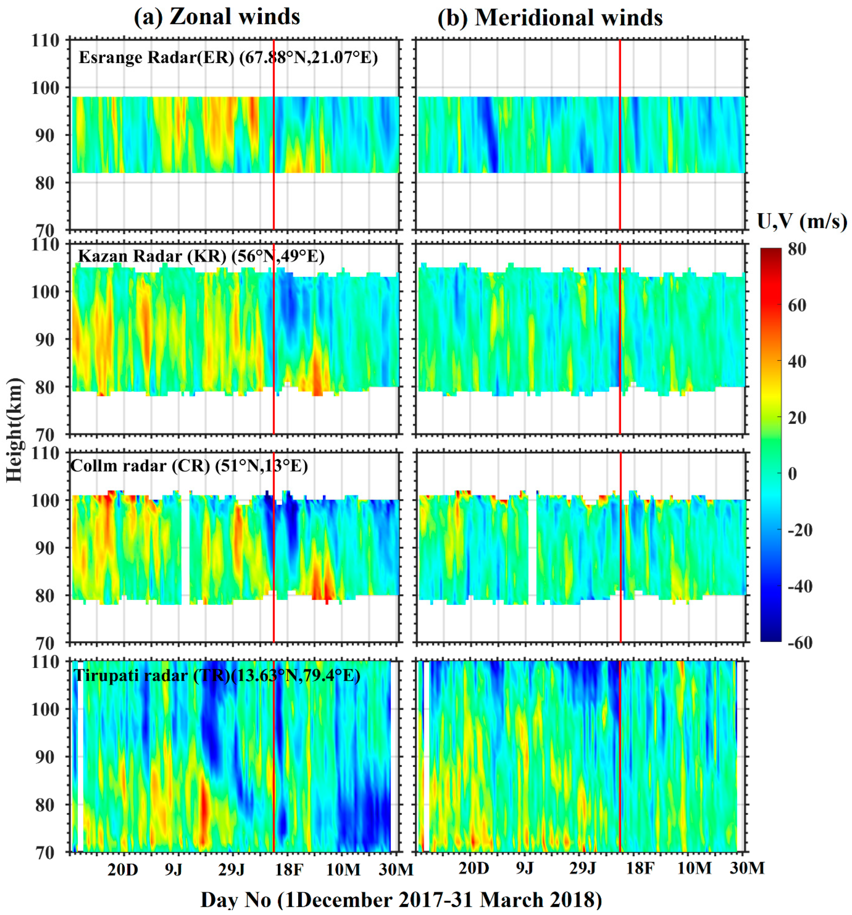
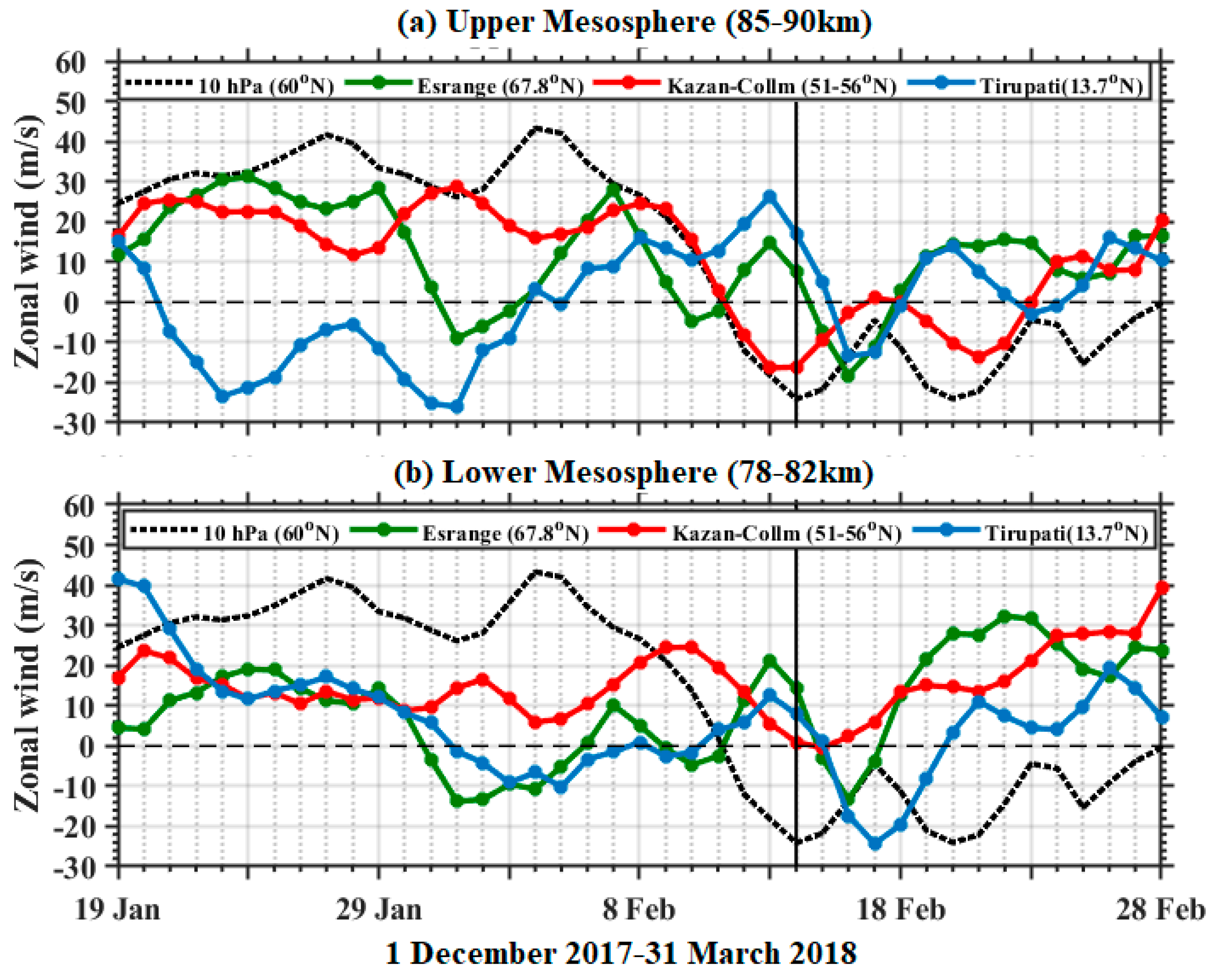
  • The zonal wind reversal in the upper mesosphere (85–90 km) occurred on the peak SSW day in mid-latitudes with a maximum value of ~(−16) m/s, whereas in tropical- and high-latitude regions, the reversal occurred two days after the SSW day with a peak value of −13 m/s and −18 m/s, respectively. In the lower mesosphere (78–82 km), the mid-latitude zonal winds weakened but did not reverse; however, in the tropical/polar regions, the reversal started two weeks before the SSW day and attained a peak value (~−24 m/s and −13 m/s) three and two days after the SSW, respectively. Hence, the highest zonal wind reversal during 2018 SSW was noted in the tropical lower mesosphere with a maximum value of ~−24 m/s.
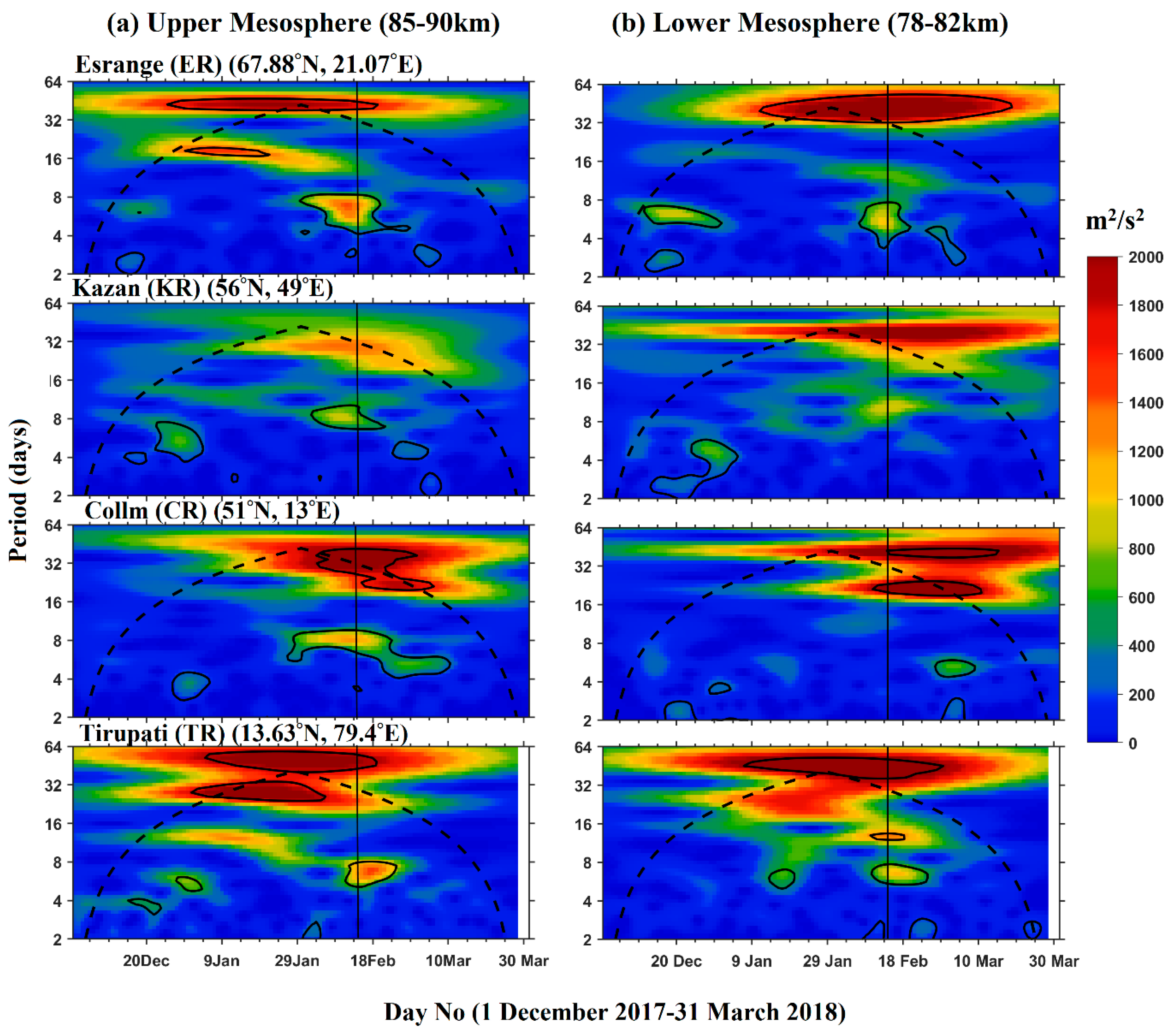
  • The wavelet analysis of zonal winds both in the upper and lower mesosphere at the four observational stations shows the presence of a wide spectrum of PWs (~2–4 days, 8 days, and 12–16 days) and waves with an intra-seasonal period (30–60-day) oscillations. The signatures of 16-day waves at the polar and 12–14-day PWs in the tropical region in the upper mesosphere were observed well before the SSW but dissipated before the peak SSW. The 8-day PWs were observed at all the stations in the upper mesosphere during the SSW, while in the lower mesosphere, they presented only at the tropical and polar stations and disappeared at the mid-latitudes.
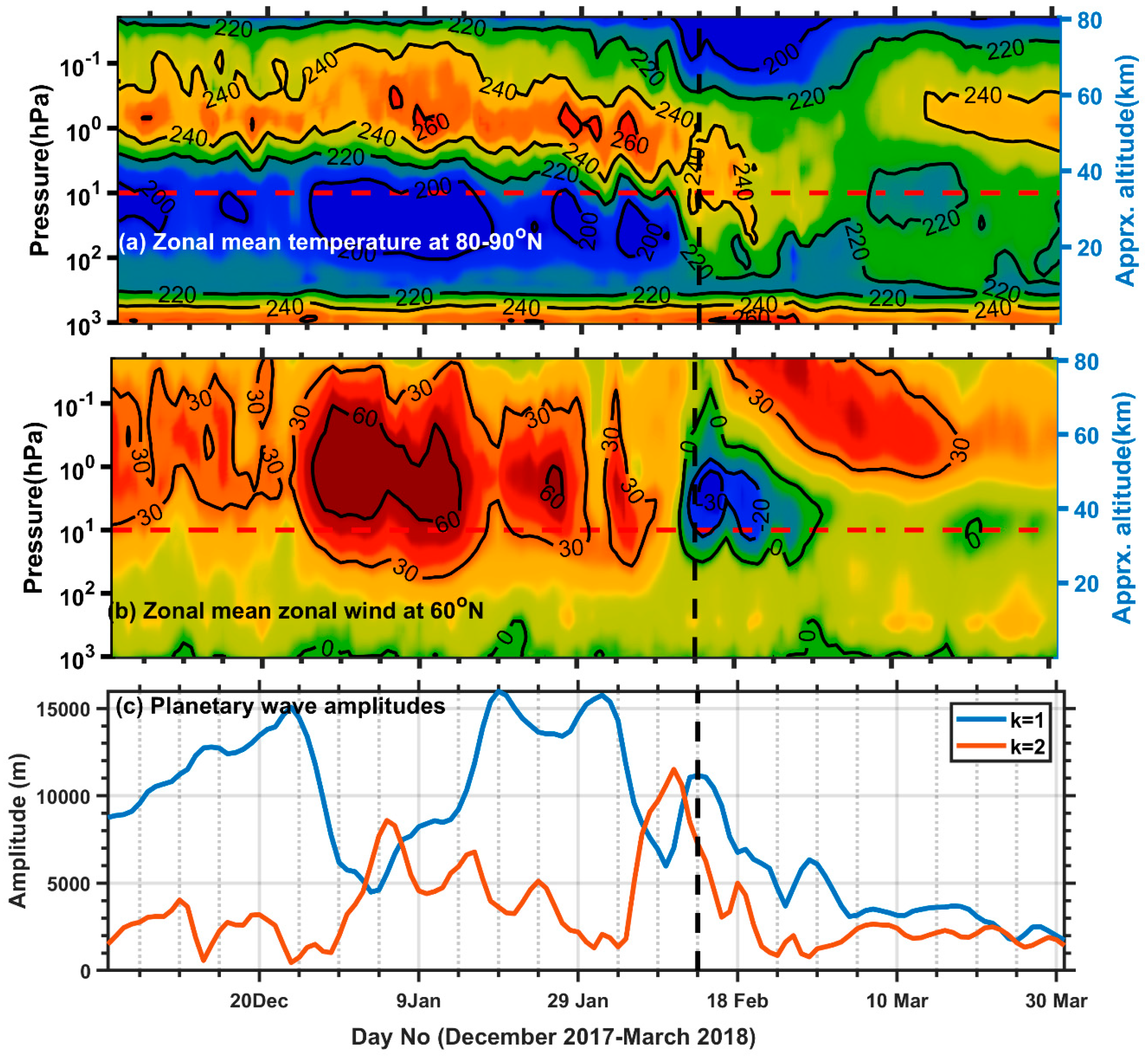
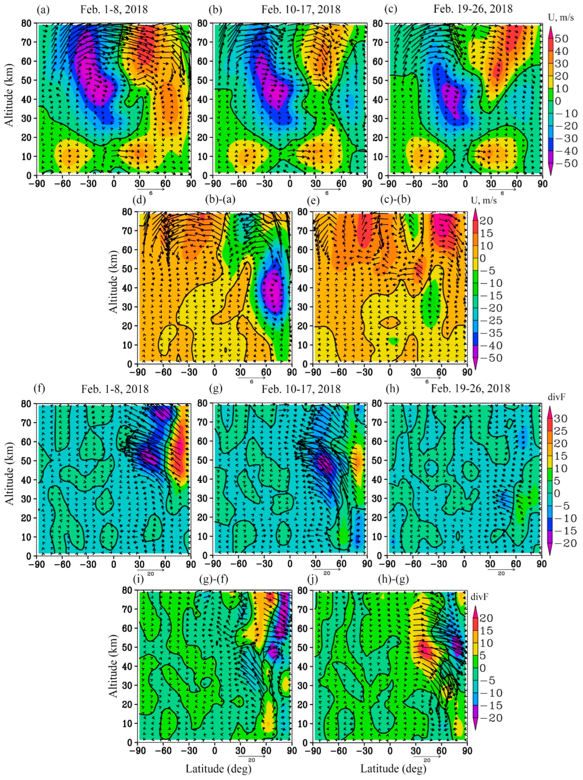
  • We estimated the residual mean meridional circulation (RMC) and EP fluxes using UKMO data at different SSW stages showing a reversal of the RMC in the mesosphere during SSW, which contributes to the cooling of this area. Additionally, the increased PW activity in the stratosphere during the SSW contributes to the zonal polar vortex breakup and additional heating of the polar region.
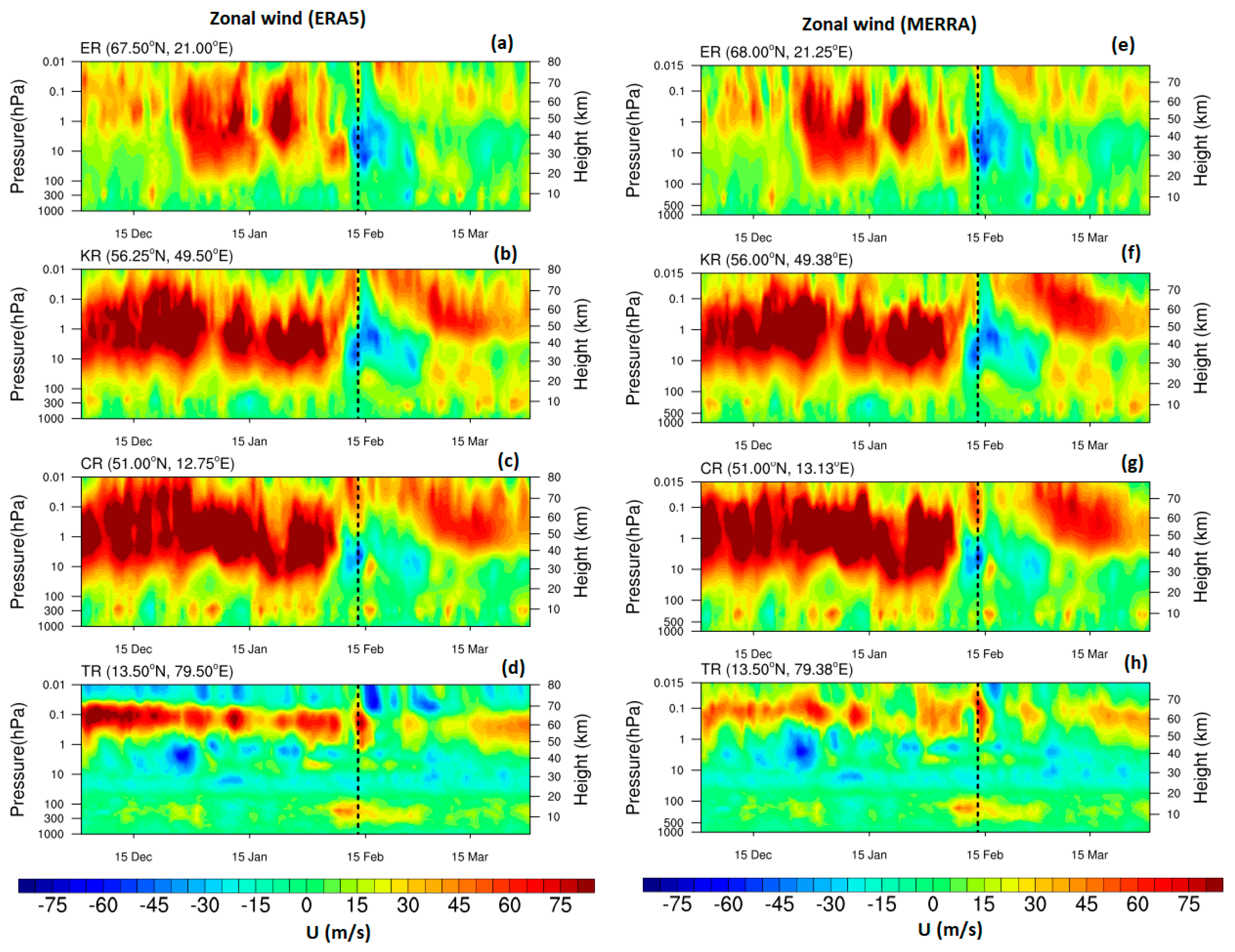
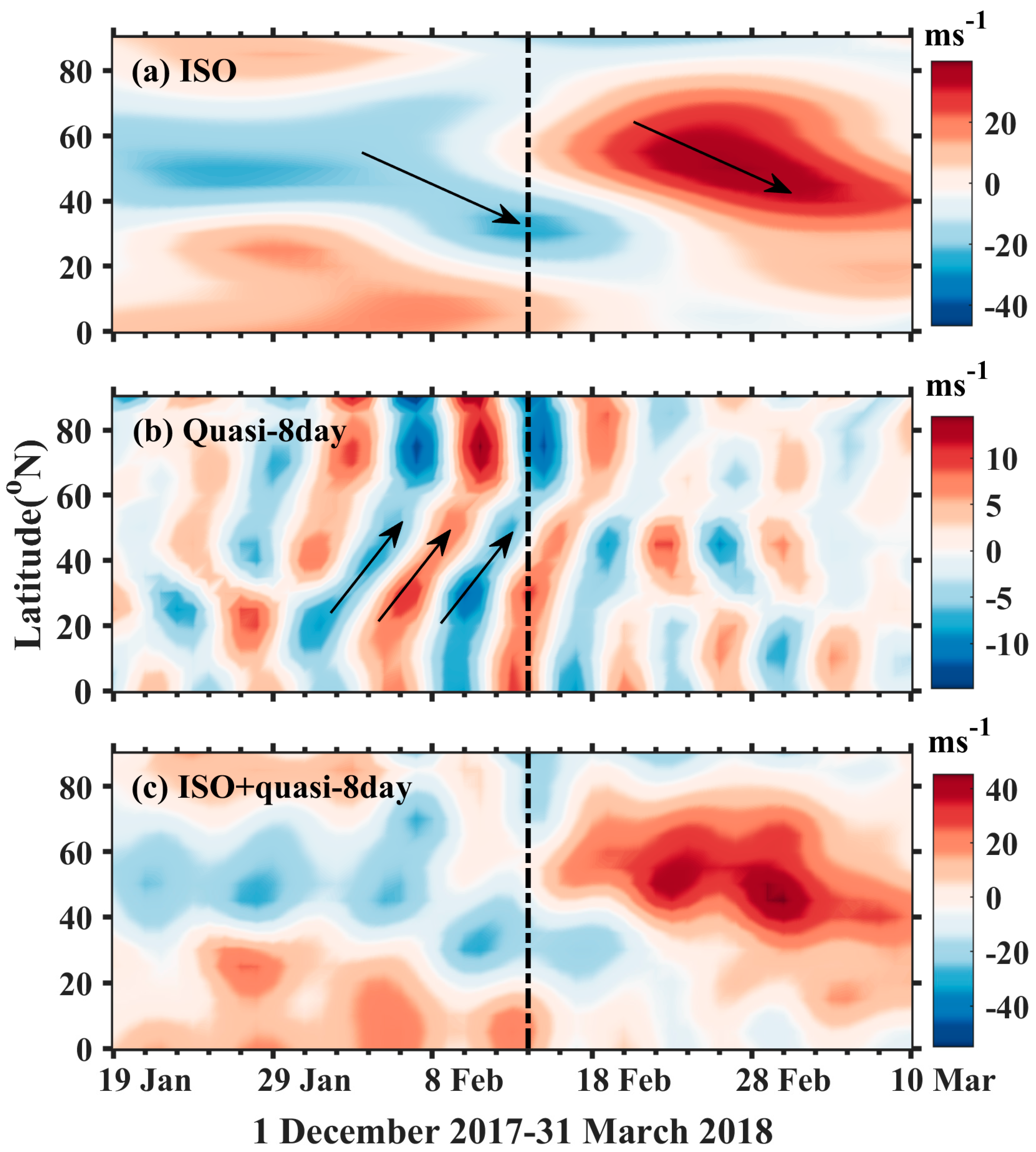
  • The radar observations showed that the ISOs were observed before the peak SSW at all stations in the upper and lower mesosphere; however, at the mid-latitudes, they attained peak amplitude after the SSW day. The latitudinal propagation of both ISOs and 8-day waves using ERA5 suggests that the ISO phase propagated to low latitudes (up to 20° N) from 60° N, before the SSW. A reverse phase propagation of the 8-day PWs was observed from the tropical to the polar regions. The superposition of this opposite phase propagation results in wind reversal in the mesosphere. The ISO and 8-day wave composite showed significant effects on the mesosphere wind reversal at the polar, mid-, and low latitudes in different time intervals and caused the delay of wind reversal both at the polar and tropical stations.
  • The ISO propagation from 60° N to tropical regions during the SSW shows an indication of a reversed mean mesosphere meridional circulation during the SSW, which is in agreement with the estimated mean meridional circulation.
Although several theoretical studies have proposed changes in the mean meridional circulation during major SSW events, observational evidence in the mesosphere is very sparse. The present study, using the MR network and reanalysis data, revealed the impact of the 2018 major SSW at the tropical and extra-tropical stations and observed changes in the PWs and ISO propagation, including changes in the mean meridional circulation. Further studies are required to address the latitudinal and longitudinal propagation of ISOs in the upper mesosphere, using multiple observations and model simulations.

Author Contributions

Conceptualization, data curation, and writing—original draft preparation, S.E., K.N.K., K.-H.S., M.V.R., E.M., C.J., S.V.B.R., N.J.M. and Y.-H.K.; methodology, S.E.; software, validation, and formal analysis, S.E., A.V.K., C.K.M., H.L., Y.-S.K. and G.V.C.; investigation, S.E., K.N.K., K.-H.S. and A.V.K.; resources, K.-H.S.; funding acquisition, K.-H.S. All authors have read and agreed to the published version of the manuscript.

Funding

The work was supported by a National Research Foundation of Korea (NRF) grant funded by the Korean government (MSIP) (No. NRF-2020R1A2C2009414) and the Korea Meteorological Administration (KMA) Research and Development Program under grant KMI2021–0141. Collm and Kazan wind observations were supported by DFG through the grant JA 836/38-1 and by RFBR through the grant 18-505-12048. RMC and EP flux calculations were supported by the Ministry of Science and Higher Education of the Russian Federation (FSZU-2023-0002) RFBR through the grant 20-77-10006.

Institutional Review Board Statement

Not applicable.

Informed Consent Statement

Not applicable.

Data Availability Statement

The MR network data can be accessed with the following DOI link: https://doi.org/10.5281/zenodo.3690723 (accessed on 12 August 2023). The authors also thank the ERA5 and MERRA-2 team for providing the wind and temperature data used in the present study. The ERA5 datasets provided by the European Centre for Medium-Range Weather Forecasts (ECMWF) are publicly available at: https://www.ecmwf.int/en/forecasts/datasets (accessed on 12 August 2023). The MERRA-2 dataset can be obtained from https://disc.gsfc.nasa.gov/datasets/M2I6NVANA_5.12.4/summary (accessed on 12 August 2023). The UK Met Office data can be obtained at https://www.metoffice.gov.uk/research/climate/maps-and-data/data/index (accessed on 12 August 2023).

Acknowledgments

We thank all the technical and scientific team operating all the meteor radars used in the present study. Additionally, we thank the funding agencies who supported this work.

Conflicts of Interest

The authors declare no conflict of interest.

References

  1. Scherhag, R. Die explosionsartige Stratosphärenerwärmung des Spätwinters 1951–1952. Ber. Dtsch. Wetterd. 1952, 6, 51–53. [Google Scholar]
  2. Matsuno, T. A dynamical model of the stratospheric sudden warming. J. Atmos. Sci. 1971, 28, 1479–1494. [Google Scholar] [CrossRef]
  3. Baldwin, M.P.; Ayarzagüena, B.; Birner, T.; Butchart, N.; Butler, A.H.; Charlton-Perez, A.J.; Domeisen, D.I.V.; Garfinkel, C.I.; Garny, H.; Gerber, E.P.; et al. Sudden Stratospheric Warmings. Rev. Geophys. 2021, 59, e2020RG000708. [Google Scholar] [CrossRef]
  4. Shi, C.; Xu, T.; Guo, D.; Pan, Z. Modulating Effects of Planetary Wave 3 on a Stratospheric Sudden Warming Event in 2005. J. Atmos. Sci. 2017, 74, 1549–1559. [Google Scholar] [CrossRef]
  5. Pedatella, N.M.; Chau, J.L.; Schmidt, H.; Goncharenko, L.P.; Stolle, C.; Hocke, K.; Harvey, V.L.; Funke, B.; Siddiqui, T.A. How Sudden Stratospheric Warming Affects the Whole Atmosphere. Eos 2018, 99. [Google Scholar] [CrossRef]
  6. Garfinkel, C.I.; Son, S.-W.; Song, K.; Aquila, V.; Oman, L.D. Stratospheric variability contributed to and sustained the recent hiatus in Eurasian winter warming. Geophys. Res. Lett. 2017, 44, 374–382. [Google Scholar] [CrossRef] [PubMed]
  7. Karpechko, A.Y.; Charlton-Perez, A.; Balmaseda, M.; Tyrrell, N.; Vitart, F. Predicting Sudden Stratospheric Warming 2018 and Its Climate Impacts with a Multimodel Ensemble. Geophys. Res. Lett. 2018, 45, 13538–13546. [Google Scholar] [CrossRef]
  8. Butler, A.H.; Gerber, E.P. Optimizing the Definition of a Sudden Stratospheric Warming. J. Clim. 2018, 31, 2337–2344. [Google Scholar] [CrossRef]
  9. Butler, A.H.; Sjoberg, J.P.; Seidel, D.J.; Rosenlof, K.H. A sudden stratospheric warming compendium. Earth Syst. Sci. Data 2017, 9, 63–76. [Google Scholar] [CrossRef]
  10. van Loon, H.; Jenne, R.L.; Labitzke, K. Zonal harmonic standing waves. J. Geophys. Res. 1973, 78, 4463–4471. [Google Scholar] [CrossRef]
  11. Krüger, K.; Naujokat, B.; Labitzke, K. The Unusual Midwinter Warming in the Southern Hemisphere Stratosphere 2002: A Comparison to Northern Hemisphere Phenomena. J. Atmos. Sci. 2005, 62, 603–613. [Google Scholar] [CrossRef]
  12. Eswaraiah, S.; Kim, Y.H.; Hong, J.; Kim, J.-H.; Ratnam, M.V.; Chandran, A.; Rao, S.; Riggin, D. Mesospheric Signatures Observed during 2010 Minor Stratospheric Warming at King Sejong Station (62° S, 59° W). J. Atmos. Sol.-Terr. Phys. 2016, 140, 55–64. [Google Scholar] [CrossRef]
  13. Eswaraiah, S.; Kim, Y.H.; Liu, H.; Ratnam, M.V.; Lee, J. Do Minor Sudden Stratospheric Warmings in the Southern Hemisphere (SH) Impact Coupling between Stratosphere and Mesosphere-Lower Thermosphere (MLT) like Major Warmings? Earth Planets Space 2017, 69, 119. [Google Scholar] [CrossRef]
  14. Eswaraiah, S.; Kim, Y.H.; Lee, J.; Ratnam, M.V.; Rao, S.V.B. Effect of Southern Hemisphere Sudden Stratospheric Warmings on Antarctica Mesospheric Tides: First Observational Study. J. Geophys. Res. Space Phys. 2018, 123, 2127–2140. [Google Scholar] [CrossRef]
  15. Eswaraiah, S.; Kim, J.; Lee, W.; Hwang, J.; Kumar, K.N.; Kim, Y.H. Unusual Changes in the Antarctic Middle Atmosphere During the 2019 Warming in the Southern Hemisphere. Geophys. Res. Lett. 2020, 47, e2020GL089199. [Google Scholar] [CrossRef]
  16. Lee, W.; Song, I.; Kim, J.; Kim, Y.H.; Jeong, S.; Eswaraiah, S.; Murphy, D.J. The Observation and SD-WACCM Simulation of Planetary Wave Activity in the Middle Atmosphere During the 2019 Southern Hemispheric Sudden Stratospheric Warming. J. Geophys. Res. Space Phys. 2021, 126, e2020JA029094. [Google Scholar] [CrossRef]
  17. Lim, E.-P.; Hendon, H.H.; Butler, A.H.; Thompson, D.W.J.; Lawrence, Z.D.; Scaife, A.A.; Shepherd, T.G.; Polichtchouk, I.; Nakamura, H.; Kobayashi, C.; et al. The 2019 Southern Hemisphere Stratospheric Polar Vortex Weakening and Its Impacts. Bull. Am. Meteorol. Soc. 2021, 102, E1150–E1171. [Google Scholar] [CrossRef]
  18. Fahimi, S.; Ahmadi-Givi, F.; Farahani, M.M.; Meshkatee, A.H. Investigation of the relationship between Euro-Atlantic and West Asia blockings and major stratospheric sudden warmings in the period of 1959–2018. Dyn. Atmos. Oceans 2021, 95, 101245. [Google Scholar] [CrossRef]
  19. Butler, A.H.; Lawrence, Z.D.; Lee, S.H.; Lillo, S.P.; Long, C.S. Differences between the 2018 and 2019 stratospheric polar vortex split events. Q. J. R. Meteorol. Soc. 2020, 146, 3503–3521. [Google Scholar] [CrossRef]
  20. White, I.P.; Lu, H.; Mitchell, N.J.; Phillips, T. Dynamical Response to the QBO in the Northern Winter Stratosphere: Signatures in Wave Forcing and Eddy Fluxes of Potential Vorticity. J. Atmos. Sci. 2015, 72, 4487–4507. [Google Scholar] [CrossRef]
  21. Laskar, F.I.; Chau, J.L.; Stober, G.; Hoffmann, P.; Hall, C.M.; Tsutsumi, M. Quasi-biennial oscillation modulation of the middle- and high-latitude mesospheric semidiurnal tides during August-September. J. Geophys. Res. Space Phys. 2016, 121, 4869–4879. [Google Scholar] [CrossRef]
  22. Lu, H.; Hitchman, M.H.; Gray, L.J.; Anstey, J.A.; Osprey, S.M. On the role of Rossby wave breaking in the quasi-biennial modulation of the stratospheric polar vortex during boreal winter. Q. J. R. Meteorol. Soc. 2020, 146, 1939–1959. [Google Scholar] [CrossRef]
  23. Andrews, D.G.; Holton, J.R.; Leovy, C.B. Middle Atmosphere Dynamics; Academic Press: San Diego, CA, USA, 1987; 489p. [Google Scholar]
  24. Laskar, F.I.; McCormack, J.P.; Chau, J.L.; Pallamraju, D.; Hoffmann, P.; Singh, R.P. Interhemispheric Meridional Circulation During Sudden Stratospheric Warming. J. Geophys. Res. Space Phys. 2019, 124, 7112–7122. [Google Scholar] [CrossRef]
  25. Rao, J.; Garfinkel, C.I.; White, I.P. Predicting the Downward and Surface Influence of the February 2018 and January 2019 Sudden Stratospheric Warming Events in Subseasonal to Seasonal (S2S) Models. J. Geophys. Res. Atmos. 2020, 125, e2019JD031919. [Google Scholar] [CrossRef] [PubMed]
  26. Kumar, K.N.; Sharma, S.K.; Joshi, V.; Ramkumar, T. Middle atmospheric planetary waves in contrasting QBO phases over the Indian low latitude region. J. Atmos. Sol. -Terr. Phys. 2019, 193, 105068. [Google Scholar] [CrossRef]
  27. Vargin, P.N.; Kiryushov, B.M. Major Sudden Stratospheric Warming in the Arctic in February 2018 and Its Impacts on the Troposphere, Mesosphere, and Ozone Layer. Russ. Meteorol. Hydrol. 2019, 44, 112–123. [Google Scholar] [CrossRef]
  28. Chandran, A.; Collins, R.L. Stratospheric sudden warming effects on winds and temperature in the middle atmosphere at middle and low latitudes: A study using WACCM. Ann. Geophys. 2014, 32, 859–874. [Google Scholar] [CrossRef]
  29. Liu, H.; Jin, H.; Miyoshi, Y.; Fujiwara, H.; Shinagawa, H. Upper atmosphere response to stratosphere sudden warming: Local time and height dependence simulated by GAIA model. Geophys. Res. Lett. 2013, 40, 635–640. [Google Scholar] [CrossRef]
  30. Liu, H.; Miyoshi, Y.; Miyahara, S.; Jin, H.; Fujiwara, H.; Shinagawa, H. Thermal and dynamical changes of the zonal mean state of the thermosphere during the 2009 SSW: GAIA simulations. J. Geophys. Res. Space Phys. 2014, 119, 6784–6791. [Google Scholar] [CrossRef]
  31. Stober, G.; Kuchar, A.; Pokhotelov, D.; Liu, H.; Liu, H.-L.; Schmidt, H.; Jacobi, C.; Baumgarten, K.; Brown, P.; Janches, D.; et al. Interhemispheric differences of mesosphere–lower thermosphere winds and tides investigated from three whole-atmosphere models and meteor radar observations. Atmos. Meas. Tech. 2021, 21, 13855–13902. [Google Scholar] [CrossRef]
  32. Satterfield, E.A.; Waller, J.A.; Kuhl, D.D.; Hodyss, D.; Hoppel, K.W.; Eckermann, S.D.; McCormack, J.P.; Ma, J.; Fritts, D.C.; Iimura, H.; et al. Statistical Parameter Estimation for Observation Error Modeling: Application to Meteor Radars. In Data Assimilation for Atmospheric, Oceanic and Hydrologic Applications (Vol. IV); Park, S.K., Xu, L., Eds.; Springer: Cham, Switzerland, 2022. [Google Scholar] [CrossRef]
  33. Quiroz, R.S. The Warming of the Upper Stratosphere in February 1966 and the Associated Structure of the Mesosphere. Mon. Wea. Rev. 1969, 97, 541–552. [Google Scholar] [CrossRef]
  34. Jacobi, C.; Kürschner, D.; Muller, H.; Pancheva, D.; Mitchell, N.; Naujokat, B. Response of the mesopause region dynamics to the February 2001 stratospheric warming. J. Atmos. Sol. -Terr. Phys. 2003, 65, 843–855. [Google Scholar] [CrossRef]
  35. Hoffmann, P.; Singer, W.; Keuer, D.; Hocking, W.; Kunze, M.; Murayama, Y. Latitudinal and longitudinal variability of mesospheric winds and temperatures during stratospheric warming events. J. Atmos. Sol. -Terr. Phys. 2007, 69, 2355–2366. [Google Scholar] [CrossRef]
  36. Zülicke, C.; Becker, E. The structure of the mesosphere during sudden stratospheric warmings in a global circulation model. J. Geophys. Res. Atmos. 2013, 118, 2255–2271. [Google Scholar] [CrossRef]
  37. Medvedeva, I.; Semenov, A.; Pogoreltsev, A.; Tatarnikov, A. Influence of sudden stratospheric warming on the mesosphere/lower thermosphere from the hydroxyl emission observations and numerical simulations. J. Atmos. Sol. -Terr. Phys. 2019, 187, 22–32. [Google Scholar] [CrossRef]
  38. Luo, J.; Gong, Y.; Ma, Z.; Zhang, S.; Zhou, Q.; Huang, C.; Huang, K.; Yu, Y.; Li, G. Study of the Quasi 10-Day Waves in the MLT Region During the 2018 February SSW by a Meteor Radar Chain. J. Geophys. Res. Space Phys. 2021, 126, e2020JA028367. [Google Scholar] [CrossRef]
  39. Shepherd, M.; Wu, D.; Fedulina, I.; Gurubaran, S.; Russell, J.; Mlynczak, M.; Shepherd, G. Stratospheric warming effects on the tropical mesospheric temperature field. J. Atmos. Sol. -Terr. Phys. 2007, 69, 2309–2337. [Google Scholar] [CrossRef]
  40. Sathishkumar, S.; Sridharan, S.; Jacobi, C. Dynamical response of low-latitude middle atmosphere to major sudden stratospheric warming events. J. Atmos. Sol. -Terr. Phys. 2009, 71, 857–865. [Google Scholar] [CrossRef]
  41. Eswaraiah, S.; Ratnam, M.V.; Kim, Y.H.; Kumar, K.N.; Chalapathi, G.V.; Ramanajaneyulu, L.; Lee, J.; Prasanth, P.V.; Thyagarajan, K.; Rao, S. Advanced meteor radar observations of mesospheric dynamics during 2017 minor SSW over the tropical region. Adv. Space Res. 2019, 64, 1940–1947. [Google Scholar] [CrossRef]
  42. Vineeth, C.; Pant, T.K.; Sridharan, R. Equatorial counter electrojets and polar stratospheric sudden warmings—A classical example of high latitude-low latitude coupling? Ann. Geophys. 2009, 27, 3147–3153. [Google Scholar] [CrossRef]
  43. Rao, S.V.B.; Eswaraiah, S.; Ratnam, M.V.; Kosalendra, E.; Kumar, K.K.; Kumar, S.S.; Patil, P.T.; Gurubaran, S. Advanced meteor radar installed at Tirupati: System details and comparison with different radars. J. Geophys. Res. Atmos. 2014, 119, 11893–11904. [Google Scholar] [CrossRef]
  44. Wang, Y.; Shulga, V.; Milinevsky, G.; Patoka, A.; Evtushevsky, O.; Klekociuk, A.; Han, W.; Grytsai, A.; Shulga, D.; Myshenko, V.; et al. Winter 2018 major sudden stratospheric warming impact on midlatitude mesosphere from microwave radiometer measurements. Atmos. Meas. Tech. 2019, 19, 10303–10317. [Google Scholar] [CrossRef]
  45. Liu, G.; Huang, W.; Shen, H.; Aa, E.; Li, M.; Liu, S.; Luo, B. Ionospheric Response to the 2018 Sudden Stratospheric Warming Event at Middle- and Low-Latitude Stations Over China Sector. Space Weather. 2019, 17, 1230–1240. [Google Scholar] [CrossRef]
  46. Shi, Y.; Shulga, V.; Ivaniha, O.; Wang, Y.; Evtushevsky, O.; Milinevsky, G.; Klekociuk, A.; Patoka, A.; Han, W.; Shulga, D. Comparison of Major Sudden Stratospheric Warming Impacts on the Mid-Latitude Mesosphere Based on Local Microwave Radiometer CO Observations in 2018 and 2019. Remote Sens. 2020, 12, 3950. [Google Scholar] [CrossRef]
  47. Matthias, V.; Stober, G.; Kozlovsky, A.; Lester, M.; Belova, E.; Kero, J. Vertical Structure of the Arctic Spring Transition in the Middle Atmosphere. J. Geophys. Res. Atmos. 2021, 126, e2020JD034353. [Google Scholar] [CrossRef]
  48. Wang, Y.; Milinevsky, G.; Evtushevsky, O.; Klekociuk, A.; Han, W.; Grytsai, A.; Antyufeyev, O.; Shi, Y.; Ivaniha, O.; Shulga, V. Planetary Wave Spectrum in the Stratosphere–Mesosphere during Sudden Stratospheric Warming 2018. Remote Sens. 2021, 13, 1190. [Google Scholar] [CrossRef]
  49. Li, N.; Luan, X.; Lei, J.; Bolaji, O.S.; Owolabi, C.; Chen, J.; Xu, Z.; Li, G.; Ning, B. Variations of Mesospheric Neutral Winds and Tides Observed by a Meteor Radar Chain Over China During the 2013 Sudden Stratospheric Warming. J. Geophys. Res. Space Phys. 2020, 125, e2019JA027443. [Google Scholar] [CrossRef]
  50. Ma, Z.; Gong, Y.; Zhang, S.; Zhou, Q.; Huang, C.; Huang, K.; Yu, Y.; Li, G.; Ning, B.; Li, C. Responses of Quasi 2 Day Waves in the MLT Region to the 2013 SSW Revealed by a Meteor Radar Chain. Geophys. Res. Lett. 2017, 44, 9142–9150. [Google Scholar] [CrossRef]
  51. Koushik, N.; Kumar, K.K.; Ramkumar, G.; Subrahmanyam, K.V.; Hocking, W.K.; He, M.; Latteck, R. Planetary waves in the mesosphere lower thermosphere during stratospheric sudden warming: Observations using a network of meteor radars from high to equatorial latitudes. Clim. Dyn. 2020, 54, 4059–4074. [Google Scholar] [CrossRef]
  52. Korotyshkin, D.; Merzlyakov, E.; Sherstyukov, O.; Valiullin, F. Mesosphere/lower thermosphere wind regime parameters using a newly installed SKiYMET meteor radar at Kazan (56° N, 49° E). Adv. Space Res. 2019, 63, 2132–2143. [Google Scholar] [CrossRef]
  53. Jacobi, C.; Arras, C.; Geißler, C.; Lilienthal, F. Quarterdiurnal signature in sporadic E occurrence rates and comparison with neutral wind shear. Ann. Geophys. 2019, 37, 273–288. [Google Scholar] [CrossRef]
  54. Mitchell, N.J.; Pancheva, D.; Middleton, H.R.; Hagan, M.E. Mean winds and tides in the Arctic mesosphere and lower thermosphere. J. Geophys. Res. Atmos. 2002, 107, SIA 2-1–2-14. [Google Scholar] [CrossRef]
  55. Hersbach, H.; Bell, B.; Berrisford, P.; Hirahara, S.; Horányi, A.; Muñoz-Sabater, J.; Nicolas, J.; Peubey, C.; Radu, R.; Schepers, D.; et al. The ERA5 global reanalysis. Q. J. R. Meteorol. Soc. 2020, 146, 1999–2049. [Google Scholar] [CrossRef]
  56. Rüfenacht, R.; Baumgarten, G.; Hildebrand, J.; Schranz, F.; Matthias, V.; Stober, G.; Lübken, F.-J.; Kämpfer, N. Intercomparison of middle-atmospheric wind in observations and models. Atmos. Meas. Tech. 2018, 11, 1971–1987. [Google Scholar] [CrossRef]
  57. Tarek, M.; Brissette, F.P.; Arsenault, R. Evaluation of the ERA5 reanalysis as a potential reference dataset for hydrological modelling over North America. Hydrol. Earth Syst. Sci. 2020, 24, 2527–2544. [Google Scholar] [CrossRef]
  58. Delhasse, A.; Kittel, C.; Amory, C.; Hofer, S.; Fettweis, X. Brief Communication: Interest of a Regional Climate Model against ERA5 to Simulate the near-Surface Climate of the Greenland Ice Sheet. Cryosph. Discuss. 2019, 5, 1–12. [Google Scholar] [CrossRef]
  59. Gelaro, R.; McCarty, W.; Suárez, M.J.; Todling, R.; Molod, A.; Takacs, L.; Randles, C.A.; Darmenov, A.; Bosilovich, M.G.; Reichle, R.; et al. The Modern-Era Retrospective Analysis for Research and Applications, Version 2 (MERRA-2). J. Clim. 2017, 30, 5419–5454. [Google Scholar] [CrossRef]
  60. Swinbank, R.; O’Neill, A.; Lorenc, A.C.; Ballard, S.P.; Bell, R.S.; Ingleby, N.B.; Andrews, P.L.F.; Barker, D.M.; Bray, J.R.; Clayton, A.M.; et al. Stratospheric Assimilated Data. Tech. Rep. 2006. British Atmospheric Data Centre, Oxfordshire, UK. Available online: http://badc.nerc.ac.uk/data/assim/ (accessed on 5 June 2022).
  61. Hocking, W.; Fuller, B.; Vandepeer, B. Real-time determination of meteor-related parameters utilizing modern digital technology. J. Atmos. Sol. -Terr. Phys. 2001, 63, 155–169. [Google Scholar] [CrossRef]
  62. Holdsworth, D.A.; Reid, I.M.; Cervera, M.A. Buckland Park All-Sky Interferometric Meteor Radar. Radio Sci. 2004, 39, 1–12. [Google Scholar] [CrossRef]
  63. Koval, A.V.; Chen, W.; Didenko, K.A.; Ermakova, T.S.; Gavrilov, N.M.; Pogoreltsev, A.I.; Toptunova, O.N.; Wei, K.; Yarusova, A.N.; Zarubin, A.S. Modelling the residual mean meridional circulation at different stages of sudden stratospheric warming events. Ann. Geophys. 2021, 39, 357–368. [Google Scholar] [CrossRef]
  64. Kozubek, M.; Lastovicka, J.; Krizan, P. Comparison of Key Characteristics of Remarkable SSW Events in the Southern and Northern Hemisphere. Atmosphere 2020, 11, 1063. [Google Scholar] [CrossRef]
  65. Jacobi, C. 6 year mean prevailing winds and tides measured by VHF meteor radar over Collm (51.3° N, 13.0° E). J. Atmos. Sol. -Terr. Phys. 2012, 78–79, 8–18. [Google Scholar] [CrossRef]
  66. Kumar, G.K.; Ratnam, M.V.; Patra, A.K.; Rao, V.V.M.J.; Rao, S.V.B.; Kumar, K.K.; Gurubaran, S.; Ramkumar, G.; Rao, D.N. Low-latitude mesospheric mean winds observed by Gadanki mesosphere-stratosphere-troposphere (MST) radar and comparison with rocket, High Resolution Doppler Imager (HRDI), and MF radar measurements and HWM93. J. Geophys. Res. Atmos. 2008, 113, 1–12. [Google Scholar] [CrossRef]
  67. Sharma, A.; Gaikwad, H.; Ratnam, M.V.; Gurav, O.; Ramanjaneyulu, L.; Chavan, G.; Sathishkumar, S. Diurnal, monthly and seasonal variation of mean winds in the MLT region observed over Kolhapur using MF radar. J. Atmos. Sol. -Terr. Phys. 2018, 169, 91–100. [Google Scholar] [CrossRef]
  68. Xiao, C.; Hu, X.; Zhang, X.; Zhang, D.; Wu, X.; Gong, X.; Igarashi, K. Interpretation of the mesospheric and lower thermospheric mean winds observed by MF radar at about 30° N with the 2D-SOCRATES model. Adv. Space Res. 2007, 39, 1267–1277. [Google Scholar] [CrossRef]
  69. Zhou, B.; Xue, X.; Yi, W.; Ye, H.; Zeng, J.; Chen, J.; Wu, J.; Chen, T.; Dou, X. A Comparison of MLT Wind between Meteor Radar Chain and SD-WACCM Results. Earth Planet. Phys. 2022, 6, 451–464. [Google Scholar] [CrossRef]
  70. Kodera, K. Influence of stratospheric sudden warming on the equatorial troposphere. Geophys. Res. Lett. 2006, 33, 1–4. [Google Scholar] [CrossRef]
  71. Eguchi, N.; Kodera, K. Impact of the 2002, Southern Hemisphere, Stratospheric Warming on the Tropical Cirrus Clouds and Convective Activity. Geophys. Res. Lett. 2007, 34, 1–5. [Google Scholar] [CrossRef]
  72. Manney, G.L.; Lawrence, Z.D.; Santee, M.L.; Read, W.G.; Livesey, N.J.; Lambert, A.; Froidevaux, C.; Pumphrey, H.C.; Schwartz, M.J. A minor sudden stratospheric warming with a major impact: Transport and polar processing in the 2014/2015 Arctic winter. Geophys. Res. Lett. 2015, 42, 7808–7816. [Google Scholar] [CrossRef]
  73. Torrence, C.; Compo, G.P.A. Practical Guide to Wavelet Analysis. Bull. Am. Meteorol. Soc. 1998, 79, 61–78. [Google Scholar] [CrossRef]
  74. Jacobi, C.; Samtleben, N.; Stober, G. Meteor radar observations of mesopause region long-period temperature oscillations. Adv. Radio Sci. 2016, 14, 169–174. [Google Scholar] [CrossRef]
  75. Matthias, V.; Hoffmann, P.; Rapp, M.; Baumgarten, G. Composite analysis of the temporal development of waves in the polar MLT region during stratospheric warmings. J. Atmos. Sol. -Terr. Phys. 2012, 90–91, 86–96. [Google Scholar] [CrossRef]
  76. Lawrence, Z.D.; Perlwitz, J.; Butler, A.H.; Manney, G.L.; Newman, P.A.; Lee, S.H.; Nash, E.R. The Remarkably Strong Arctic Stratospheric Polar Vortex of Winter 2020: Links to Record-Breaking Arctic Oscillation and Ozone Loss. J. Geophys. Res. Atmos. 2020, 125, e2020JD033271. [Google Scholar] [CrossRef]
  77. Giarnetti, S.; Leccese, F.; Caciotta, M. Non recursive multi-harmonic least squares fitting for grid frequency estimation. Measurement 2015, 66, 229–237. [Google Scholar] [CrossRef]
  78. Qin, Y.; Gu, S.; Dou, X. A New Mechanism for the Generation of Quasi-6-Day and Quasi-10-Day Waves During the 2019 Antarctic Sudden Stratospheric Warming. J. Geophys. Res. Atmos. 2021, 126, e2021JD035568. [Google Scholar] [CrossRef]
  79. Gong, Y.; Xue, J.; Ma, Z.; Zhang, S.; Zhou, Q.; Huang, C.; Huang, K.; Li, G. Observations of a Strong Intraseasonal Oscillation in the MLT Region During the 2015/2016 Winter Over Mohe, China. J. Geophys. Res. Space Phys. 2022, 127, e2021JA030076. [Google Scholar] [CrossRef]
  80. Niranjankumar, K.; Ramkumar, T.K.; Krishnaiah, M. Vertical and lateral propagation characteristics of intraseasonal oscillation from the tropical lower troposphere to upper mesosphere. J. Geophys. Res. Atmos. 2011, 116. [Google Scholar] [CrossRef]
Figure 1. Geographical locations of the meteor radar network used in the present study.
Atmosphere 14 01302 g001
Figure 2. Day–altitude cross-sections of the (a) daily mean polar cap temperature at 80–90° N and (b) daily zonal mean zonal wind at 60° N obtained from ERA5. The approximate height of the corresponding pressure level is displayed on the right axis. (c) Planetary wave (k = 1 and k = 2) amplitudes at 10 hPa and 60° N. The vertical dashed lines indicate the day of peak warming, whereas the dashed horizontal lines in (a,b) indicate the 10 hPa pressure level. The eastward winds are shown with ‘red’ color and westward winds with ‘blue’color. The +ve values of the zonal wind refer to the eastward and –ve values of the zonal wind are the westward directions.
Atmosphere 14 01302 g002
Figure 3. (a) Day–height contour of the daily mean zonal wind obtained from 1 December 2017 to 31 March 2018, using Esrange radar (ER) at 68° N, Kazan meteor radar (KR) at 56° N, Collm meteor radar (CR) at 51° N, and Tirupati meteor radar (TR) at 14° N (top to bottom). (b) Same as (a) but shows the meridional winds. The vertical lines indicate the SSW day.
Atmosphere 14 01302 g003
Figure 4. Day–height contours of the daily mean zonal winds obtained from ERA5 (ad) and MERRA (eh) data from 1 December 2017 to 31 March 2018, near meteor radar locations. The vertical line indicates the SSW day.
Atmosphere 14 01302 g004
Figure 5. Daily mean variability of the averaged zonal winds (solid lines) (a) in the upper mesosphere (85–90 km) and in the (b) lower mesosphere (78–82 km) obtained using the meteor radar network. Daily mean zonal winds at 10 hPa, 60° N are shown by a dotted black line. The dashed horizontal line indicates the zero-wind level, and the vertical line indicates the SSW day.
Atmosphere 14 01302 g005
Figure 6. Continuous wavelet spectra of the averaged zonal winds in the (a) upper mesosphere (85–90 km) and (b) lower mesosphere (78–82 km) observed by the meteor radar network. The dashed curved black lines in the wavelet spectra show the respective cone of influence, and the vertical lines show the SSW day.
Atmosphere 14 01302 g006
Figure 7. (a) Latitude–height distributions of zonal winds (m/s) (color contour) and the residual mean meridional circulation (RMC) components (m/s) (vector) before SSW (1–8 February 2018). (b) Same as (a) but during the SSW (10–17 February 2018). (c) Same as (a) but after the SSW (19–26 February 2018). (d,e) Changes between the specified parameters ((b–a,c–b), respectively). (fj) Correspond to (ae) but for the EP flux divergence (102 m2/s/day, shaded) and EP flux components (108 m3/s2, arrows). The vertical component was multiplied by 200 for the sake of illustration.
Atmosphere 14 01302 g007
Figure 8. (a) The 30–60-day filtered intra-seasonal oscillations (ISOs) of the zonal wind at 80 km using ERA5 data. (b) Same as (a) but for the 8-day wave, and (c) shows the composite of both ISOs and 8-day waves. The filtered oscillations were obtained for the zonal wind in the longitudes in the range of 10–100° E (covering all meteor radar longitudes). The dashed vertical lines show the SSW day.
Atmosphere 14 01302 g008
Table 1. Main features of the meteor radars used in this study.
TirupatiCollmKazanEsrange
(13.5° N, 79.4° E)(51° N, 13° E) (56° N, 49° E) (67° N, 21° E)
Freequency35.25 MHz36.2 MHz29.75 MHz32.5 MHz
Peak Power40 kW40 kW15 kW6 kW
PRF430 Hz430 Hz1590 Hz2144 Hz
Altitude coverage70–110 km70–110 km80–105 km80–98 k
Disclaimer/Publisher’s Note: The statements, opinions and data contained in all publications are solely those of the individual author(s) and contributor(s) and not of MDPI and/or the editor(s). MDPI and/or the editor(s) disclaim responsibility for any injury to people or property resulting from any ideas, methods, instructions or products referred to in the content.

