The 50th Anniversary of the Metaphorical Butterfly Effect since Lorenz (1972): Multistability, Multiscale Predictability, and Sensitivity in Numerical Models

Abstract

Lorenz rediscovered the butterfly effect, which is defined as the sensitive dependence on initial conditions (SDIC), in 1963. In 1972, he used the term “butterfly” as a metaphor to illustrate how a small perturbation can lead to a tornado with a complex structure. The metaphorical butterfly effect, which celebrated its 50th anniversary in 2022, is not precisely the same as the original butterfly effect with SDIC. To commemorate the 50th anniversary, a Special Issue was launched and invited the submission of research and review articles that can help to enhance our understanding of both the original and metaphorical butterfly effects. The Special Issue also sought recent developments in idealized Lorenz models and real-world models that address multistability, multiscale predictability, and sensitivity. The call for papers was opened 15 months prior to the completion of the Special Issue and features nine selected papers. This editorial provides a brief review of Lorenz models, introduces the published papers, and summarizes each one of them.

1. Introduction

A well-accepted definition of the butterfly effect is the sensitive dependence on initial conditions (SDIC), which was rediscovered by Lorenz in 1963 (Lorenz 1963a) [1]. Usage of the term “butterfly” appeared in 1972 when Lorenz applied a metaphor to discuss the possibility of whether a tiny perturbation may eventually create a tornado with a three-dimensional, organized coherent structure (Lorenz 1972 [2]). Since 1972, the metaphorical butterfly effect has received increasing attention and has become associated with the SDIC. Lorenz’s work in 1963 and 1972 established the foundation for chaos theory, inspiring many studies in different fields. The metaphorical butterfly effect celebrated its 50th anniversary in 2022 (Glick 1987 [3]; Lorenz 1993 [4]).

Although Lorenz’s 1963 theoretical model is considered a toy weather model that cannot accurately depict weather and climate, the model’s simplicity allowed for the identification of chaotic weather and climate, leading to the widely accepted view that weather is chaotic. The announcement of the 2019 Nobel Physics Prize cited Lorenz’s pioneering chaos study as a foundation for the awarded studies, which proposed physics-based mathematical models for improving our understanding of predictability in complex systems [5]. The proposed physics-based mathematical models are capable of revealing crucial, fundamental physical processes, including co-existing rapidly and slowly varying systems and the metastability of spin glass [6]. By extending Lorenz’s 1963 model in order to improve our understanding of predictability in complex systems such as weather and climate, which possess co-existing attractors [7], Shen et al. (2021a, b) [8,9] proposed a revised view in that “weather possesses chaos and order; it includes emerging organized systems (such as tornadoes) and recurrent seasons”, in contrast to the conventional view of “weather is chaotic”.

To celebrate the 50th anniversary of the metaphorical butterfly effect and to promote fundamental research through the use of both theoretical and real-world modeling, as well as modern machine learning technology, a Special Issue was established, seeking investigations into various topics related to multistability, multiscale predictability, and sensitivity. These topics included:

• The validity of existing analogies and metaphors for butterfly effects.
• The insightful analysis of various Lorenz models reveals the role of monostability with single types of solutions and multistability with attractor co-existence in contributing to the multiscale predictability of weather and climate.
• The development of conceptual, theoretical, and real-world models to reveal fundamental physical processes and multiscale interactions that contribute to our understanding of the butterfly effect on the predictability of weather and climate.
• Innovative machine learning methods that (1) classify chaotic and non-chaotic processes and identify weather and climate systems at various spatial and temporal scales (e.g., sub-seasonal to seasonal time scales) and (2) detect computational chaos and saturation dependence on various types of solutions.
• The impact of tiny perturbations on emergent pattern formation with self-organization (e.g., stripes and rolls), the formation of high-impact weather (e.g., tornados and hurricanes), etc.

Nine papers, covering topics related to the first four categories, were published during the 15-month period of the Special Issue. The published papers are summarized herein based on the four categories: (A) butterfly effects and sensitivities, (B) atmospheric dynamics and the application of theoretical models, (C) predictability and prediction, and (D) computational and machine learning methods.

To complement the contributions of the published papers to the goals of the Special Issue, in Section 2, we first provide a brief review of Lorenz’s models between 1960 and 2008. Further mathematical analysis of the Lorenz models can be found in a companion article by Shen (2023) [10]. Thereafter, Section 3 provides a summary of the papers. Appendix A briefly compares the mathematical similarities of the Lorenz 12-variable model [4] and the many-mode model, and Appendix B documents the relationship between the logistic map and the logistic differential equation used by Lorenz in the 1960s. For detailed definitions of the selected concepts, please refer to

Table A1. Definitions of the selected concepts included in the Special Issue.

Name	Definitions	Recommendations
First kind of attractor co-existence	The co-existence of chaotic and steady-state solutions.	[7,8,9,160]
Second kind of attractor co-existence	The co-existence of nonlinear oscillatory and steady-state solutions.	[7,8,9]
Analogues	Analogues are two states of the atmosphere that exhibit resemblance to each other.	[21]
Attractor	The smallest attracting point set that, itself, cannot be decomposed into two or more subsets with distinct basins of attraction.	[8]
Butterfly effect (BE), general	The phenomenon in that a small alteration in the state of a dynamical system will cause subsequent states to differ greatly from the states that would have followed without the alteration.	[4]
BE of the first kind (BE1)	The sensitive dependence on initial conditions (SDICs).	[1,4,139]
BE of the second kind (BE2)	The capability of a small disturbance to create an organized circulation at large distances.	[2,4,139]
BE of the third kind (BE3)	(1)  The hypothetical role of small-scale processes in contributing to finite predictability; (2)  Ill-conditioning and instability.	[139,140,157]
BE in Saiki and Yorke (2023)	Instability in high-dimensional linear systems.	[155]
Chaos	Bounded aperiodic orbits exhibit a sensitive dependence on ICs.	[4,159]
Final state sensitivity	Nearby orbits settle to one of multiple attractors for a finite but arbitrarily long time.	[82]
Intransitivity	A specific type of solution lasts forever.	[52,72]
Monostability	The appearance of single-type solutions.	[159]
Multistability	A system with multistability contains more than one bounded attractor that only depends on ICs.	[159]
Quasi-periodicity	A quasi-periodic solution consists of two or more incommensurate frequencies, the ratios of which are irrational.	[91]
Recurrence	This refers to a trajectory returning to the vicinity of its previous location.	[92,93]
Sensitive dependence	The property characterizing an orbit if most other orbits that pass close to it at some point do not remain close to it as time advances.	[4]
Ventilation coefficient parameterization	A parameter used in numerical models of atmospheric convection to represent the effect of environmental wind on convective updrafts.	[156]

in Appendix C.

2. A Brief Review of Lorenz Models and Butterfly Effects

2.1. A Review of Lorenz Models

In this paper, we provide an overview of Prof. Lorenz’s mathematical models that illustrate chaotic and unstable features in the atmosphere. The primary emphasis is on models that present two key concepts, namely chaos and almost intransitivity (for further details, please refer to Table A1 in Appendix C), both of which are related to predictability. Lorenz published 61 papers during his lifetime, with 58 of them being single authored (Chen 2020 [11]).

Table 1. A list of Lorenz models in the 1960s. * By a strict definition, the Lorenz 1969 model cannot be categorized as a turbulence model, but it does illustrate the multiscale turbulent features of the Atmosphere.

Year	1960	1960/62	1963	1964	1965	1969	1969
Equations	3 ODEs,	12 ODEs	3 ODEs,	Logistic map	28 variables	Logistic ODE	21 2nd-order ODEs,
Origins	PDE; vorticity Eq	PDEs; a 2-layer, QG model	PDEs; convection		PDEs; a 2-layer, QG model		PDE; vorticity Eq
Features of Solutions	oscillatory solutions with elliptic functions	irregular fluctuations	chaos	steady, periodic, non-periodic	irregular solutions	error growth and saturation	‘turbulence’ *

and

Table 2. A list of Lorenz models between 1970 and 2008.

Year	1972	1976	1980	1984	1986	1996/2006	2005	2008
Equations	turbulence models	cubic map	low-order PE or QG (9 or 3) ODEs	3 ODEs	5 or 3 ODEs	N ODEs	N ODEs	Henon map
Origins	PDE based		PDE based	Not PDE based	PDE based, (the 1980 model)	Not PDE based	Not PDE based
Features of Solutions	turbulence	transitivity	(modified) shallow water Eqs.	general circulation, transitivity	slow manifolds (w elliptic functions)	chaos	chaos	chaos

summarize his mathematical models in the 1960s and between 1970 and 2008, respectively.

2.1.1. Lorenz Models in the 1960s

In 1960, Lorenz proposed a low-order system of ordinary differential equations (ODEs) based on a single partial differential equation (PDE) for the conservation of vorticity (Lorenz 1960 [12]). This system, called Maximum Simplification of the Dynamic Equations, produced oscillatory solutions as elliptic functions ([12,13]). As discussed below, Lorenz’s 1960 model also appeared as a simplified version of the Lorenz 1986 system for studying slow variables. In the same year, Lorenz reported “irregular solutions” based on a system of twelve ODEs, derived from the geostrophic form of the two-layer baroclinic model, which is discussed below. The system includes two variables that represent the average and the difference of the stream functions for the two layers. The second variable was identified as the temperature field through the thermal wind relationship. To express each variable, six Fourier modes with six coefficients were used, resulting in a system of twelve ODEs with twelve mathematical variables but only two physical fields (i.e., a stream function and temperature). The mathematical equations are presented in Equation (A1) in Appendix A. In 1960, Lorenz presented the “irregular solutions”, which were later published in a conference proceeding in 1962 [14], at the International Symposium on Numerical Weather Prediction in Tokyo.

Motivated by the irregular solutions observed within the Lorenz (1960/1962) model, Lorenz simplified the Saltzman seven-variable model [15,16] into a three-variable model, which is known as the Lorenz 1963 model with three ODEs [1,17]. Since then, thanks to its rich array of features, the model has been valuable in explaining the nonlinear and chaotic dynamics of diverse fields [1,3,4].

Within a continuous dynamical system, three ODEs are required for the appearance of chaos. While the Lorenz 1963 model represents one such simple system for producing chaos, a simple logistic map (which is a difference equation) has also been used to illustrate chaos (e.g., May 1976 [18]; Li and Yorke 1975 [19]). Although cited in [18], Lorenz (1964) [20], indeed, applied the logistic map in order to illustrate irregular solutions earlier than May (1976). Lorenz (1964) specifically reported the transition from steady-state to periodic to non-periodic behavior as the control parameter increases. Simply based on the findings of Lorenz (1962, 1963a, and 1964), we may conclude that Lorenz was fully aware of the potential of Saltzman’s model in illustrating chaos. As compared to the logistic map in a discrete form, the continuous form of the logistic equation was applied in order to illustrate the monotonic increase and the saturation of errors (e.g., Lorenz 1969a [21]). The relationship between the logistic map and the logistic ODE is briefly documented in Appendix B.

The aforementioned low-order models were constructed in order to illustrate various atmospheric phenomena which are intrinsically nonlinear (Lorenz 1982a [22]). During the early 1960s, numerous multi-layer models existed. One of the two-layer models was developed by Lorenz in 1960 (Lorenz 1960 [23]). The geostrophic form of the two-layer model was applied in order to derive the Lorenz 1962 8-variable model [24] and the Lorenz 1960/1962 12-variable model and it was subsequently changed to become a 14-variable model for investigating vacillation in a dishpan, as described in Lorenz’s work in 1963 (Lorenz 1963b [25]). Within the eight-variable model, Lorenz was able to obtain analytical solutions to describe essential features of the transition between the Hadley and Rossby regimes. Building upon these endeavors, Lorenz proposed a 28-variable model in 1965 to explore non-periodic solutions (Lorenz 1965 [26]). The four quasi-geostrophic (QG) models are also referred to as the Lorenz 1962-8v, 1960/1962-12v, 1963-14v, and 1965-28v models. Whilst the 1960/1962-12v model and the 1965-28v model are listed in Table 1, the Lorenz 1960 two-layer model, the 1962-8v model, and the 1963-14v model are not listed in Table 1.

The Lorenz 1965 28-variable model is a highly simplified QG model used for capturing some of the gross features of atmospheric behavior and contains two physical variables, the stream function (i.e., vorticity) and potential temperature. This model yielded a significant finding of flow-dependent predictability: “The time required for errors comparable to observational errors in the atmosphere to grow to intolerable errors is strongly dependent upon the current circulation pattern, and varies from a few days to a few weeks.” This finding implies that the predictability limit depends on a synoptic situation (Lorenz 1982b [27]). In fact, some results obtained using the 28-variable model were also reported in Lorenz (1963c) [28].

While this review primarily focuses on the features of Lorenz models, it is worth mentioning the following important “analysis method.” In Lorenz (1965), the growth of small errors, such as during the linear stage, was analyzed using the singular value (SV) method (Kalnay 2002 [29]; Lewis 2005 [30]). This method required the calculation of the system’s Jacobian matrix (for a linear tangent model) and its singular values (for growth rates). Such a method was applied to determine the local or finite-time Lyapunov exponent over a finite time interval (Nese 1989 [31]; Abarbanel et al., 1992 [32]; Eckhardt and Yao 1993 [33]; Krishnamurthy 1993 [34]; Szunyogh et al. 1997 [35]; Yoden 2007 [36]). On the other hand, Oseledec (1968) [37] independently proposed a general approach for calculating the (global) Lyapunov exponent over an infinite time interval. The singular value method was also employed in the systems of the European Centre for Medium-Range Weather Forecasts (ECMWF) (Molteni et al., 1996 [38]; Buizza et al., 2008 [39]). In a recent study conducted by Cui and Shen (2021) [40], the relationship between the SV decomposition (SVD), principal component analysis (PCA), and kernel PCA methods was documented. Furthermore, they deployed kernel PCA to identify co-existing attractors within the phase space. Empirical orthogonal function (EOF), which was initially introduced into the field of meteorology by Lorenz in 1956 [41], is another term commonly used to denote PCA.

A two-layer, quasi-geostrophic model was also applied by Pedlosky in the 1970s, referred to as the Pedlosky model (Pedlosky 1971, 1972, 1987 [42,43,44]), in order to derive a low-order system to study nonlinear baroclinic waves. Although the Pedlosky and Lorenz 1963 models were derived from very different PDEs with different physical processes, research indicates that two systems of ODEs can be mathematically identical when time-independent parameters are properly selected (Pedlosky and Frenzen, 1980 [45]; Shen 2021 [46]). Similar to the Lorenz 1963 model, the Pedlosky model also produced three types of solutions, including steady-state, chaotic, and limit cycle solutions.

2.1.2. Lorenz Models between 1970 and 2008

While Lorenz 1963 has been highly cited within the nonlinear dynamics community, the Lorenz 1969 many-mode model (Lorenz 1969b [47]) is better known by individuals within the meteorology community. Similar to the Lorenz 1960 model, the Lorenz 1969 model was also derived based on the conservation of vorticity. Since the conservative PDE does not include friction, as compared to the turbulence models proposed by Leith 1971 [48], Leith and Kraichnan (1972) [49], and Lorenz himself in 1972 [50,51], the Lorenz 1969 model is not a turbulence model. Thus, while the Lorenz 1963 model was simplified from the Saltzman model in order to qualitatively illustrate the chaotic nature of the atmosphere, the Lorenz 1969 model was proposed to qualitatively illustrate multiscale interactions of the “turbulent” atmosphere. As a result of its importance, as summarized in Section 3, detailed features of the Lorenz 1969 model have recently been documented. To illustrate the concept of “intransitivity” highlighted in Section 2.1.3, Lorenz (1976) [52] employed a cubic map. This cubic map can be obtained by substituting a cubic term for a quadratic term in Equation (B4), as found in Appendix B.

Based on a shallow water equation, Lorenz 1980 [53] obtained a low-order system of nine ODEs, referred to as the nine-variable barotropic primitive-equation (PE) model (Lorenz 1982a [22]), to describe the evolution of the velocity potential, stream function, and the height of a free surface. By applying a quasi-geostrophic assumption, Lorenz showed that a simplified version of the low-order system can be mathematically identical to the Lorenz 1963 model. In 1986, by applying the Lorenz 1980 low-order system, Lorenz (1986) [54] proposed a system of five ODEs in order to illustrate the features of the slow manifold. Using different initial conditions, Lorenz discussed two types of solutions: (1) a linear gravity wave solution for two fast variables and (2) a nonlinear Rossby wave with a dependence of oscillatory frequency on the amplitude of the wave for three slow variables, U, V, and W. As a result, the term “slow” indicates a state of the system where time scales are sufficiently separated and fast gravity modes are effectively separated. Both solutions are non-chaotic. Lorenz (1986) did not present the concept of co-existing chaotic and non-chaotic solutions. For a detailed discussion on the absence of universal slow-manifold evolution in rotating stratified fluids, the readers may find the studies by Lorenz and Krishnamurthy (1987) [55], Lorenz (1992) [56], and McWilliams (2019) [57] of interest. These studies delve into the subject matter and provide further insights.

Table 3. A comparison of the Lorenz 1986 model for slow variables with two simplified versions of the Lorenz 1963 model (Sparrow 1982 [58]; Shen 2018 [59]).

	The Lorenz (1986) Model	The Limiting Equations	The Non-Dissipative Lorenz Model
References	Lorenz (1986)	Sparrow(1982)	Shen (2018)
Equations	$\frac{dU}{dt}=-VW,$ $\frac{dV}{dt}=UW,$ $\frac{dW}{dt}=-UV.$	$\frac{dX}{d\tau }=\sigma Y,$ $\frac{dY}{d\tau }=-XZ,$ $\frac{dZ}{d\tau }=XY.$	$\frac{dX}{d\tau }=\sigma Y,$ $\frac{dY}{d\tau }=-XZ+rX,$ $\frac{dZ}{d\tau }=XY.$
Solutions	$U=U^{*}cn\left(W^{*}T\right)$ $V=V^{*}sn\left(W^{*}T\right)$ $W=W^{*}dn\left(W^{*}T\right)$	$X=\sqrt{2\sigma }cn(\sqrt{\sigma }\tau +3K)$ nonlinear periodic orbits	three types of solutions, including two types of periodic solutions and homoclinic orbits
Remarks	$T=T\left(t\right)$	See Shen (2018) for details	See Shen (2018) for details

compares the “subsystem” of a Lorenz 1986 model for the three slow variables and two simplified versions of the Lorenz 1963 model [58,59,60]. The first two models, listed in the second and third columns, have closed-form solutions with elliptic functions, showing the modulation of frequency within nonlinear periodic solutions. Although the models can produce periodic solutions, they cannot generate limit cycle solutions because there are no dissipative terms. A limit cycle is defined as an isolated closed orbit within the phase space [8]. A system with U, V, and W variables (e.g., Table 3) is comparable to Equations (15)–(17) in Lorenz (1960)l, whose solutions are also the elliptic functions dn, sn, and cn (see Table 3).

To depict atmospheric circulation, Lorenz (1984) [61] proposed a different system of three ODEs, viewed as the simplest general circulation model (GCM). In the past, the model has been applied in order to qualitatively illustrate features of the atmosphere (e.g., chaotic winters and non-chaotic summers (Lorenz 1990 [62]), the long-term variability of the climate (Pielke and Zeng (1994) [63]), etc.). To help readers understand the validity of the model and related findings, the following comments are provided. Lorenz (1990) [62] documented that (1) the system was constructed in a somewhat ad hoc manner (i.e., a lack of physical foundations) and (2) there is no assurance that the system produces bounded solutions. Although a recent study has provided a method to derive the Lorenz 1984 model [64,65], transformations of variables made it difficult to interpret the physical meanings of variables within the 1984 system. As compared to typical, fully dissipative systems where the time change rate of the volume of the solutions is negative, the volume of the solution within the 1984 model does not necessarily shrink to zero. Specifically, Lorenz (1991) [66] stated that: (1) We do not claim or intend that it (i.e., the Lorenz 1984 model) should reproduce atmospheric behavior in any quantitative sense. (2) The point is not that the model is a good representation of the atmosphere.

Until 1996/2006, as indicated by the title of Lorenz (1996, 2006) [67,68], Lorenz acknowledged that the predictability problem has not been fully solved. While the Lorenz 1963 model is a forced, dissipative, but limited-scale model, the Lorenz 1969 model is a linear, multiscale system with no dissipations. In 1996, to discuss growth rates at different scales and their saturations, Lorenz [67] proposed a many-mode “nonlinear” model that included dissipations and forcing terms. Lorenz (1996) was a technical report and was later published as a book chapter in 2006 (Lorenz 2006 [68]). As shown in Equation (A2) in Appendix A, the system contains nonlinear quadratic terms for advection and linear terms for dissipative and forcing terms. The system produces chaotic responses. However, without providing detailed justifications for how rescaling was performed, the coefficients for all terms at all scales were one (e.g., Equation (1) in Lorenz 1996). As compared to the Lorenz 1960/1962-12v model (e.g., Equation (A1) in Appendix A) and the Lorenz 1969 model, as well as the generalized Lorenz model (Shen 2019 [7]), the coupling terms (or the nonlinear quadratic terms), which originate from mode–mode interactions, should not have the same coefficients. Similarly, coefficients for the dissipative terms should not be the same.

Although a new chaotic many-mode system was proposed in order to address the predictability problem in 1996, Lorenz rescaled the variables to make the time unit (i.e., a time scale) equal to 5 days and chose a time step of 0.05 units that is equivalent to 6 h (page 5 of Lorenz 1996). The time scale of 5 days is different from the time scale of 6 days used by Lorenz (1969b), who determined the time scale by assuming a velocity scale of 17.2 m/s. Thus, the impact of a selected time scale on the estimate of predictability horizons within idealized models (that may or may not be physics based) should be examined. While two copies of the Lorenz 1996 model (i.e., Equation (1) in Lorenz 1996 or Equation (A2) in Appendix A) were applied in order to construct a two-layer system (i.e., Equations (2) and (3) in Lorenz 1996), additional linear coupling terms were included, calling for additional justifications for the choice of linear coupling terms that should be consistent with existing nonlinear quadratic terms. Other chaotic models in Lorenz (2005) [69] shared similar pros and cons with the 1996 model. Lorenz (2006) [70] utilized the Lorenz 1996/2005 model to demonstrate the existence of regimes that occur when the external forcing parameter (e.g., F in Equation (A2)) exceeds its critical value for the onset of chaos. In the last year of his life, Lorenz (2008) [71] published a paper based on the Hénon map which is a second-order difference equation with a quadratic term. A PDE-based classification of Lorenz models is provided in

Table 4. The PDE-based classification of Lorenz models.

Quasi-geostrophic (QG) System	1962-8v, 1960/1962-12v, 1963-14v, 1965-28v
Conservative Vorticity Equation	1960, 1969
Rayleigh Benard Convection Equations	1963 (& Generalized Lorenz Models)
Shallow Water Equations	1980, 1986
No PDEs	1984, 1996, 2005
(Discrete) Maps	1964 (Logistic), 1976 (Cubic), 2008 (Henon)

.

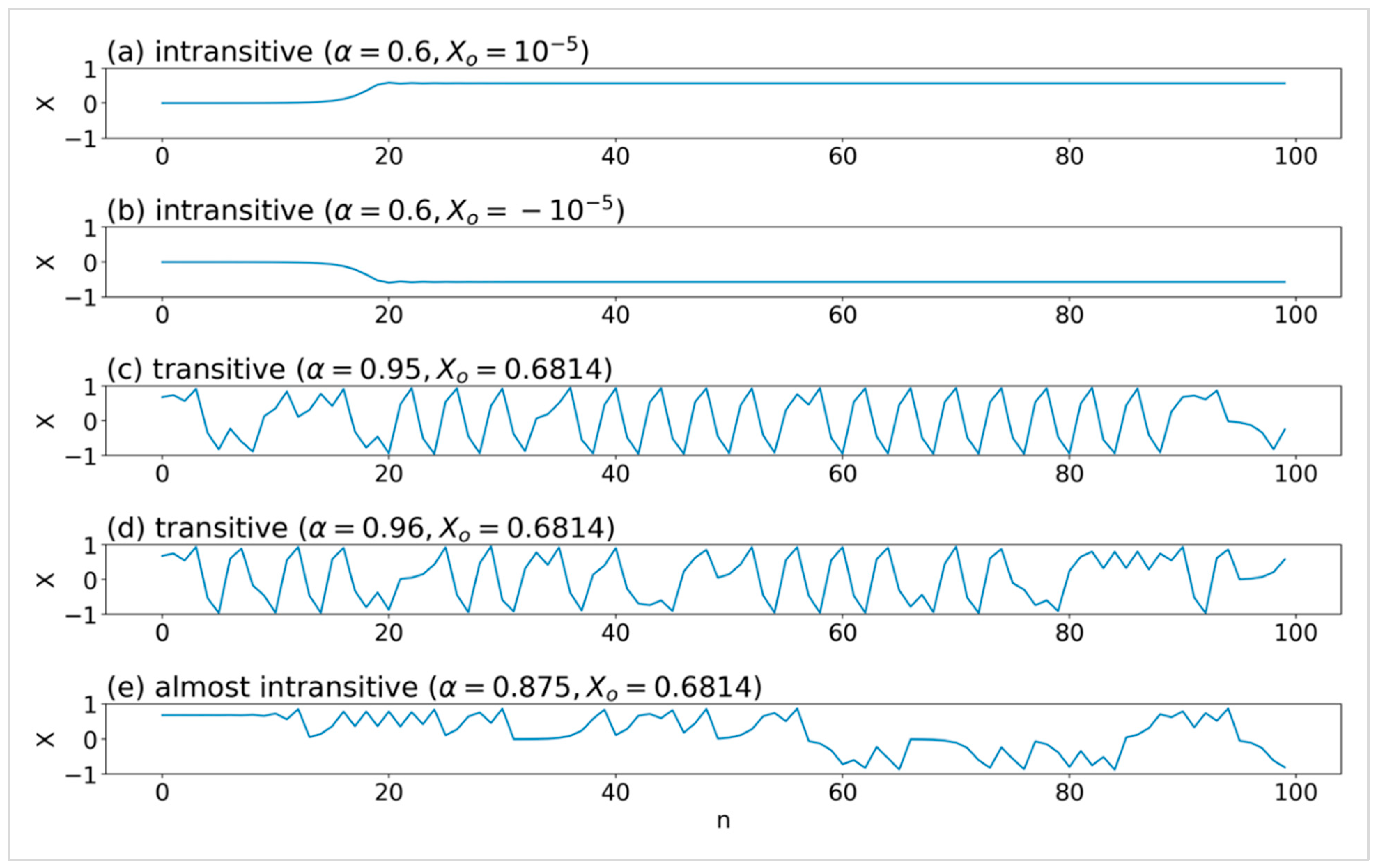
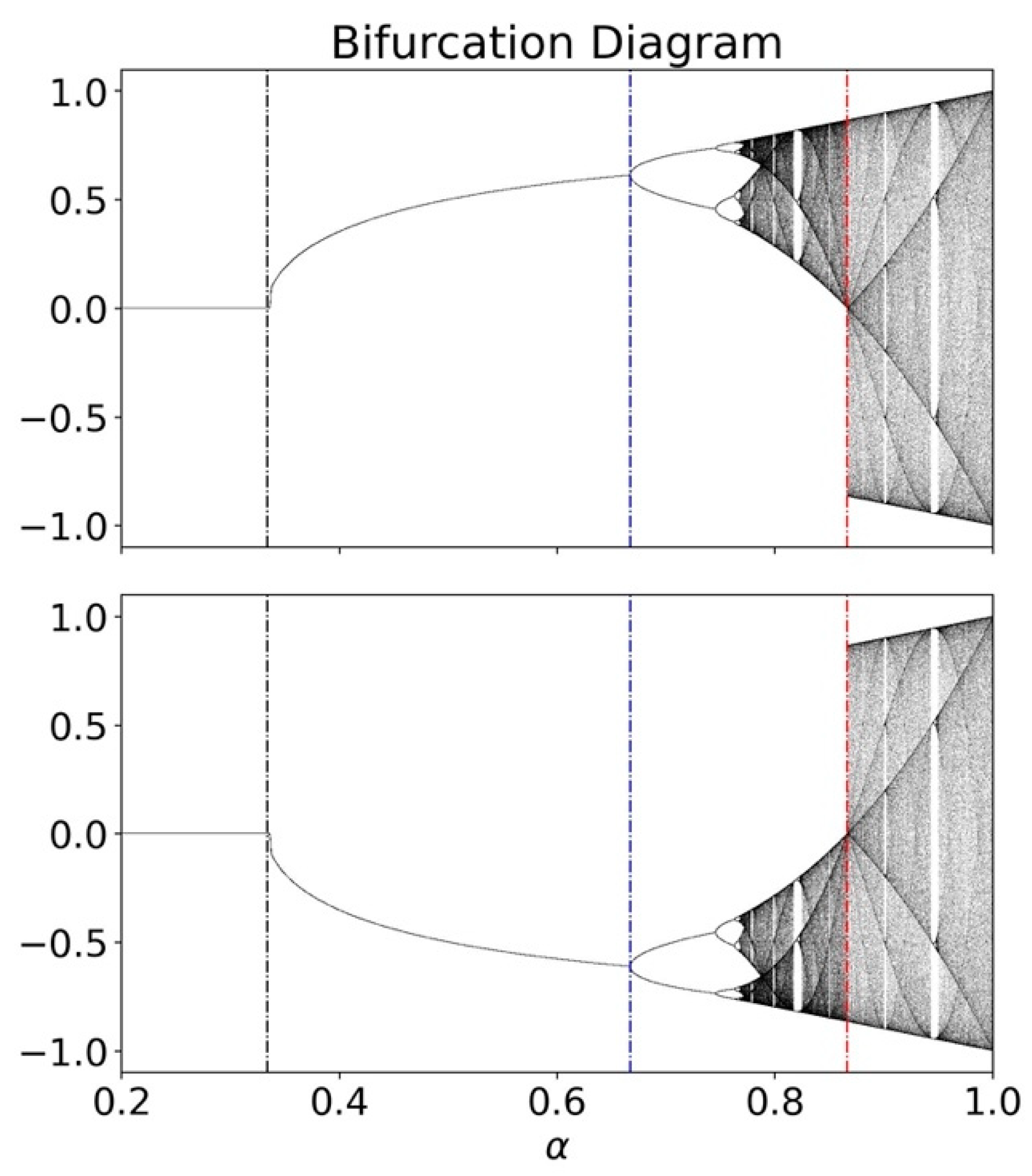
2.1.3. Transitivity, Intransitivity, and Almost Intransitivity

While chaos with SDIC and linearly unstable solutions for multiscale predictability have been well explored using Lorenz’s original models, the concept of “intransitivity” has been suggested and explored using different models since the 1960s (Lorenz, 1968 [72], 1975 [73], 1976 [52], 1982c [74], 1990 [62], and 1997 [75]). The idea of “intransitivity” addresses whether or not a specific type of weather or climate regime may last forever. In mathematical terms, the relation is classified as transitive if, whenever it establishes a link between A and B, as well as a separate link between B and C, a connection is implied between A and C. Thus, a relation is called intransitive if it is not transitive. When examining a system with two distinct states or regimes (such as warm and cold weather characterized by positive and negative temperature anomalies, respectively), if either warm or cold weather indefinitely persists, the system demonstrates “intransitivity”. In other words, transitions from one state to another state are impossible. On the other hand, if the two weather regimes are alternate, the system exhibits “transitivity”. The third scenario, known as “almost intransitivity”, occurs when a regime change is possible but happens infrequently, falling between the two aforementioned scenarios.

Therefore, drawing from the preceding information, we can observe that “transitivity”, “almost intransitivity”, and “(complete) intransitivity” are demonstrated by the occurrence of “frequent”, “rare”, and “no” changes in the signs of solutions (i.e., oscillations between two distinct regimes), correspondingly. As shown in Figure 1, these features were effectively illustrated by Lorenz (1976), who applied a cubic map, $X_{n+1}=\alpha \left(3X_n-4X_n^3\right)$ (i.e., a cubic finite difference equation, e.g., Holmes (1979) [76] and May (1984) [77]). The parameter $\alpha$ symbolizes a combined effect of linear forcing and dissipations, referred to as effective linear forcing. Additionally, the ratio between the coefficients of linear and nonlinear components determines the level of nonlinearity.

As shown in Figure 2 for the bifurcation diagram of the cubic map, when the parameter $\alpha$ is greater than 1/3, the model displays a pitchfork bifurcation that introduces two non-trivial equilibrium points. Such non-trivial equilibrium points become unstable when $\alpha$ is greater than 2/3. Then, each critical point experiences period doubling bifurcations, yielding a chaotic attractor (De Oliveira et al., 2013 [78]). Transitivity arises from the merger of two chaotic attractors [79,80] when $\alpha$ exceeds the critical threshold ${\alpha }_c=\sqrt{3}/2$. Lorenz (1976) suggested that while transitivity arises when $\alpha$ is greater than ${\alpha }_c$, almost intransitivity occurs when $\alpha$ slightly surpasses ${\alpha }_c$.

In the chaotic regime of the Lorenz 1963 model, which consists of one saddle point and two unstable equilibrium points, as evidenced by the presence of a persistent chaotic solution, the model demonstrates “transitivity” in the phase space. According to Devaney’s definition of chaos [81], topological transitivity, SDIC (sensitive dependence on initial conditions), and dense periodic orbits are the three conditions that define chaos. In comparison, the concept of “intransitivity” and “almost intransitivity” emerges as an intriguing topic within systems that allow for the co-existence of two chaotic attractors associated with two non-trivial equilibrium points (such as the Lorenz 1976 cubic map), the co-existence of two oscillatory solutions (like the Lorenz 1984 model), and/or various types of attractor co-existence (such as the generalized Lorenz model [7]).

For example, given time-independent parameters, co-existing attractors may occupy different portions of the phase space. In such cases, both transitivity and “almost intransitivity” become possible when one or more parameters change over time. According to the following description of an intransitive system by Lorenz (1968) [72]:

“There are two or more sets of long-term statistics, each of which has a greater-than-zero probability of resulting from randomly chosen initial conditions”

the intransitivity and the final state sensitivity (Grebogi et al. (1983) [82]; Table A1) are related. On the other hand, considering the presence of chaotic solutions within a transitive regime, such as those observed in the Lorenz 1963 model, whether or not “almost intransitivity” could manifest during a specific time period is an intriguing question.

When the concepts of “intransitivity” and “almost intransitivity” were initially introduced to explore the potential longevity of different climate regimes, if they exist, investigating regime changes on weather or short-term climate scales may also be valuable. For instance, Charney and DeVore (1979) [83] proposed that the presence of multiple, stable steady-state solutions in a low-order QG system could lead to the emergence of atmospheric blocking in the form of a stable steady-state solution (e.g., Chen and Xiong 2016 [84]). This phenomenon arises from the interplay of nonlinearity and mechanical and thermal forcing. Understanding the factors that govern the transitions between zonal and blocked atmospheric circulations, as well as the persistence of these regimes, remains an active area of research (Faranda et al., 2016 [85]; Dorrington and Palmer 2023 [86]). At longer time scales, transitions between El Niño and La Niña events exhibit varying durations for each regime ([87], Wallace et al. [88]), which raises scientific inquiries regarding the factors influencing the frequency and duration of these transitions. This prompts the exploration of whether the notions of “almost intransitivity” or “transitivity” can be applicable in describing such transitions and understanding the conditions (i.e., nonlinear and/or chaotic dynamics) that govern them.

2.1.4. Analogues and Recurrence

Lorenz’s models revealed the potential existence of multiple attractors, such as co-existing chaotic attractors in Lorenz (1976) and co-existing periodic oscillations in Lorenz (1984). However, despite these findings, the prevailing assumption regarding the presence of a single dominant chaotic attractor has been implicitly applied in order to explain why identical weather systems are rare (e.g., Van Den Dool 1989 and 1994 [89,90]). Such an explanation gained widespread acceptance due to the fact that neighboring trajectories in chaotic systems, such as the Lorenz 1963 model, do not interact within the phase space.

However, it is important to note that nearby oscillatory trajectories, which eventually reach a steady state, do not intersect prior to reaching their final destination. Additionally, as illustrated in Figure 3 in Faghih-Naini and Shen (2018) [91], who applied the non-dissipative five-dimensional Lorenz model, a quasi-periodic solution with multiple incommensurate frequencies does not form a closed orbit but rather a torus. Therefore, when considering the temporal and spatial variations of forcing and dissipation processes, which are often neglected in autonomous systems, it becomes essential to consider “recurrence” instead of “periodicity”. As defined in Thompson and Stewart (2002) [92] and studied using high-dimensional Lorenz models by Reyes and Shen (2019, 2020) [93,94], recurrence refers to a trajectory returning to the vicinity of its previous location. Recurrence can be seen as a more inclusive concept that encompasses quasi-periodicity with multiple frequencies and chaos.

In fact, the idea of recurrence can be compared to the quasi-periodicity introduced in Lorenz’s earlier studies during the 1960s (e.g., Lorenz 1963a and 1963c [28]). Lorenz defined a “quasi-periodic flow” as:

“A flow with no transient component eventually comes arbitrarily close to assuming a state which it has assumed before, and the history following the latter occurrence remains arbitrarily close to the history following the former.”

Additionally, the notion of “recurrence” aligns well with Lorenz’s concept of “analogues” (Lorenz 1969a [21], 1973 [95]), defined as follows:

“Analogues are two states of the atmosphere that exhibit resemblance to each other. Either state in a pair of analogues can be considered equivalent to the other state plus a small superposed ‘error’.”

While weather may not repeat itself exactly, the idea of “analogues” or “recurrence” is also consistent with the classification of various weather systems such as quasi-biennial oscillations (QBOs), atmospheric blocking, African Easterly Waves (AEWs), and others (Shen et al., 2021a,b and references therein). The natural occurrence of analogues, i.e., similar weather situations, has been applied as an empirical approach for estimating growth rates (Lorenz 1969c [96]). When two states are comparable, their differences are viewed as an error, and the growth of the error can be estimated by observing the evolution of the two states. Lorenz (1969a) reported both quasi-exponentially growing and decaying systems. While Lorenz’s analogue approach in a follow-up study (Lorenz 1973) suggested a predictability horizon of at least 12 days for instantaneous weather patterns, recent advances in nonlinear dynamics, including attractor co-existence and almost intransitivity, can serve as a basis for understanding the potential for studying predictability at sub-seasonal, seasonal, or climate scales.

2.1.5. Simplifications and Generalizations of Lorenz Models

The three primary categories of chaotic systems include Hamiltonian systems (such as the three-body problem of Poincare [97,98]), forced and dissipative differential ODEs, and difference equations (like May 1976 and Li and Yorke 1975). Lorenz models can be categorized as belonging to the second and third categories. As such, numerous studies have been conducted over the past five decades, drawing inspiration from Lorenz’s previously mentioned models. These studies have explored mathematical and physical simplifications and the generalizations of Lorenz models (e.g., Curry 1978 [99]; Curry et al., 1984 [100]; Howard and Krishnamurti 1986 [101]; Hermiz et al., 1995 [102]; Thiffeault and Horton 1996 [103]; Musielak et al., 2005 [104]; Roy and Musielak 2007a, b, c [105,106,107]; Moon et al., 2017 [108]), resulting in various noteworthy findings. Some of these include mathematical equivalence amongst the non-dissipative Lorenz 1963 model, the Korteweg–de Vries (KdV) equation in the traveling wave coordinate, the nonlinear Schrodinger equation for the amplitude of a traveling wave, the SIR model with weakly nonlinear assumptions, and the inviscid Pedlosky model (Shen 2020, 2021 [46,60]; Paxson and Shen 2022 [109]). SIR represents the three categories of individuals: susceptible (S), infected (I), and recovered (R) in that order. Consequently, such simplified systems have proven effective in revealing the dynamics of solitary waves, homoclinic orbits, epidemic waves, and nonlinear baroclinic waves. As a result of orbital instability and the unique sensitivity to initial conditions exhibited by homoclinic orbits, one could argue that the conservative, non-dissipative Lorenz 1963 model generates limited chaos.

Recently, Saiki et al. (2017) [110] proposed mathematical unification of the Lorenz 1963, 1984, and 1996 models. These systems, whether of dimension 3 or N, share quadratic characteristics and possess a generalized Lyapunov function that ensures bounded trajectories, with all trajectories entering a bounded trapping region. Furthermore, in terms of generalizing the Lorenz 1963 model, Shen (2019a, b) [7,111] proposed an expanded version that incorporates the following features: (1) any odd number of state variables greater than three, (2) the presence of three common types of solutions (steady-state, chaos, and limit cycle solutions), (3) two kinds of attractor co-existence, (4) aggregated negative feedback, (5) hierarchical spatial scale dependence, and (6) energy conservation under the dissipationless condition.

The presence of two types of attractor co-existence makes the generalized model suitable for investigating transitivity and intra-transitivity. Revealing the predictability of different attractors can be achieved through the effective detection of attractors, which involves determining their boundary (referred to as the basin boundary; Cui and Shen 2021 [40]). The concept of “edge of chaos” suggests that the interplay of chaos and order could lead to complexity as well as the emergence of self-organized phenomena [112,113]. The simplest system for illustrating the edge of chaos is the self-adjusting logistic map [114], i.e., a logistic map with a time-varying control parameter. Thus, the generalized Lorenz model with time-varying parameters can be applied to illustrate the transition between regular and chaotic solutions.

The Lorenz 1963 model revealed not only SDIC (i.e., chaos) but also the intriguing discovery of fractal geometry within its solution (Lorenz 1963a, 1993; Gleick 1987; Palmer 2009 [115]; Emanuel 2011 [116]; Feldman 2012 [117]). Fractals represent geometric objects that exhibit self-similarity. Various techniques exist for calculating fractal dimensions, employing diverse mathematical definitions and types of fractal dimensions (Grassberger and Procaccia 1983 [118]; Nese et al., 1987 [119]; Ruelle 1989 [120]; Zeng et al., 1992 [121]). One such measure is the Kaplan–Yorke dimension (Kaplan and Yorke 1987 [122]), which requires the computation of Lyapunov exponents (Wolf et al., 1985 [123]; Shen 2014 [124]). Consequently, these dimensions are influenced by system parameters, such as the Rayleigh parameter. By considering typical parameter values (e.g., Shen 2014 and 2015 [125]), the fractal dimension of the Lorenz 1963 model was determined to be 2.06, indicating a dependence amongst the three selected Fourier models. The five-, six-, and seven-variable Lorenz models were derived by extending the nonlinear feedback loop, incorporating five, six, and seven Fourier modes, respectively (commonly referred to as the five-, six-, and seven-dimensional Lorenz models, Shen 2014, 2015, and 2016 [124,125,126]). These higher-dimensional Lorenz models exhibit fractal dimensions, and the 7D or higher-dimensional Lorenz models clearly demonstrate hierarchical scale dependence (Shen 2016 and 2017 [126,127]).

2.1.6. Error Growth Analysis Using the First- and Second-Order ODEs

Throughout his entire career, Lorenz employed the logistic differential equation (e.g., Equation (A3) in Appendix B) in order to examine errors, which became known as the Lorenz error growth model (Lorenz 1969a [21], 1982 [27]; Nicolis 1992 [128], Zhang et al. (2019) [129]). This equation is a first-order ODE containing a quadratic nonlinear term (e.g., X², with X representing a variable). Lorenz (1969a) provided explanations for this nonlinear term and referred to his assumption as the quadratic hypothesis. While his analogue approach resulted in a doubling time of 8 days (Lorenz 1969a), the logistic ODE yielded an estimated doubling time of 2.5 days. To account for the disparities, he substituted the quadratic term (X²) with a cubic term (X³), which produced a different doubling time of 5 days. However, Lorenz remained cautious and acknowledged that the choice of the cubic term had less justification. In fact, later, Lorenz (1982a) suggested that results with the quadratic hypothesis are “reasonable but not readily verifiable”. Apart from discrepancies arising from different nonlinear terms (such as quadratic and cubic terms), variations can also emerge when applying different types of ODEs (with the same initial growth rate), including first and second-order ODEs.

For instance, whilst incorporating nonlinearity within a single first-order ODE can generate new equilibrium points, first-order ODEs can only exhibit a “monotonic” evolution between successive equilibrium points (Alligood et al., 1996 [130]; Meiss 2007 [131]; Strogatz 2015 [132]). The classical logistic ODE cannot reveal both quasi-exponentially growing and decaying errors reported using the analogue approach in Lorenz (1969b). In contrast, introducing nonlinearity within a single second-order ODE can yield different outcomes, leading to homoclinic orbits and/or oscillatory solutions. The X (or Z) component of the non-dissipative Lorenz 1963 model is, indeed, a second-order ODE with a cubic (or quadratic) nonlinear term.

Recent studies have documented differences in error representation between first-order and second-order ODEs using the linear system (such as the logistic equation without the quadratic term), the logistic equation (i.e., the Lorenz error growth model), and the KdV-SIR equation, which is a second-order ODE with a cubic nonlinear term (Paxson and Shen 2022 and 2023 [109,133]). Mathematically, the KdV-SIR equation is identical to the Z component of the non-dissipative Lorenz 1963 model and the Kortewegde Vries (KdV) equation in the traveling wave coordinate; it represents the epidemic SIR model under a weakly nonlinear assumption. The classical SIR model, proposed by Kermack and McKendrick (1927) [134], describes the evolution of susceptible (S), infected (I), and recovered (R) individuals. Using real-world models, the presence of oscillatory root-mean-square averaged forecast errors in ensemble runs was previously reported when oscillatory solutions prevailed over specific regions or time periods (Liu et al., 2009 [135]). Shen et al. (2010) [136] documented oscillatory correlation coefficients in 30-day simulations of multiple African easterly waves using a global mesoscale model (Shen et al., 2006a, b, [137,138]).

2.2. A Review of Butterfly Effects within Lorenz Models

Over the past five decades, various types of butterfly effects (BEs) have impacted our lives in direct or indirect ways. However, misunderstandings and misinterpretations of these effects are prevalent. In order to provide clarity and to support the goals of the Special Issue, Shen et al. (2022b) [139] define and describe the three major kinds of BEs: the sensitive dependence on initial conditions (SDIC), the ability of small disturbances to create large-scale circulation, and the hypothetical role of small-scale processes and/or instability in contributing to finite predictability [140]. These three kinds of BEs are referred to as BE1, BE2, and BE3, respectively (see Table A1 in Appendix C). In order to prevent inaccurate generalizations, understanding the physical source of energy through a brief exploration can aid in the appropriate application of related discoveries. One of the major limitations of a linear model is that its instability remains unchanged over time.

The following folklore has been a popular analogy for SDIC (i.e., the BE1) (e.g., [3,141]):

• For want of a nail, the shoe was lost.
• For want of a shoe, the horse was lost.
• For want of a horse, the rider was lost.
• For want of a rider, the battle was lost.
• For want of a battle, the kingdom was lost.
• And all for the want of a horseshoe nail.

As illustrated by Shen et al., 2022b [139], such an analogy is not accurate (e.g., Lorenz 2008 [142].) because the verse does not indicate boundedness.

2.3. A Review of Lorenz’s Perspective on the Predictability Limit

In relation to the origin of the inherent limit to predictability in the atmosphere (e.g., Charney et al. [143], GARP 1969 [144], Lorenz 1969a, b, c, d, e, 1982a, b, 1984b, 1985, 1993, and 1996 [145,146,147,148]; Smagorinsky (1969) [149]; Lighthill 1986 [150]; Lewis 2005 [30]; Rotunno and Synder 2008 [151]; Durran and Gingrich 2014 [152]; Reeve 2014 [153]; and Zhang et al., 2019 [129]), a recent literature review was conducted by Shen et al., 2023 [154] to present the following perspective as proposed by Lorenz:

A.

The Lorenz 1963 model qualitatively revealed the essence of finite predictability within a chaotic system, such as the atmosphere. However, the Lorenz 1963 model did not determine a precise limit for atmospheric predictability.

B.

In the 1960s, using real-world models, the two-week predictability limit was originally estimated based on a doubling time of 5 days. Since then, this finding has been documented in Charney et al. (1966) [143] and has become a consensus.

Further examination of predictability within the Lorenz 1963 and 1969 models was carried out by Shen et al. (2022a), with a summary provided in Section 3.

3. Overview of the Published Papers

Our summary of the papers published in the Special Issue covers four topics: (A) butterfly effects and sensitivities, (B) atmospheric dynamics and the application of theoretical models, (C) predictability and prediction, and (D) computational and machine learning methods.

3.1. (A) Butterfly Effects and Sensitivities

Saiki and Yorke (2023) [155] challenged the notion that a positive Lyapunov exponent is a necessary condition for the occurrence of a butterfly effect, which is defined as temporary exponential growth resulting from a small perturbation. A positive Lyapunov exponent refers to the rate at which two infinitesimally close trajectories diverge from each other (Wolf et al., 1985 [123]; Shen 2014 [124]). Using simple linear map models, the paper demonstrated that a butterfly effect can occur even without chaos or a positive Lyapunov exponent. Specifically, the authors examined a 24-dimensional version of the map, which exhibits a significant butterfly effect despite having a Lyapunov exponent of 0.

The paper introduced a linear “infected mosquito” model to illustrate how off-diagonal matrix entries can contribute to a finite-time growth rate. The authors suggested that the degree of instability in a system can be better characterized by its finite-time growth rate, which takes into account the impact of off-diagonal matrix entries. The study’s findings indicated that in higher-dimensional systems, off-diagonal matrix entries may have a more significant impact on a system’s behavior than Lyapunov exponents. The paper concluded that understanding the dynamics of simpler, non-meteorological models can shed light on additional aspects of the butterfly effect. By focusing on the finite-time growth rate, valuable insights into a system’s behavior can be gained, even in linear systems that lack chaos or positive Lyapunov exponents.

The study by Chou and Wang (2023) [156] investigated the sensitivity of the ventilation coefficient parameterization to the life span of a simulated storm. The authors modified the parameterization of the ventilation coefficient for different precipitation particles, such as rain, snow, and hail, and compared the results to their previous study where the ventilation effect of precipitation particles was either halved or doubled as a whole. The results indicated that changing the ventilation coefficient of rain, snow, or hail categories leads to different storm evolution paths. It was found that reducing the ventilation effect of rain leads to quick dissipation, whereas enhancing the ventilation effect of rain or snow/hail leads to the development of multicellular storms. The study additionally demonstrated the impact of changes in cloud microphysical parameterization on larger-scale dynamical processes.

3.2. (B) Atmospheric Dynamics and the Application of Theoretical Models

The study of Lewis and Lakshmivarahan (2022) [17] focused on the challenge of data assimilation in chaotic and non-chaotic regimes, specifically the placement of observations to induce convexity of the cost function in the space of control. The authors used Saltzman’s spectral model of convection, which has both chaotic and non-chaotic regimes controlled by two parameters, to examine this problem. They simplified the problem by stripping the seven-variable constraint to a three-variable constraint and used the forecast sensitivity method (FSM) to deliver sensitivities within the placement. The authors used the observability Gramian to locate observations at places that force the Gramian positive definite, and the locations were chosen such that the condition number of V^T V was small and guaranteed convexity in the vicinity of the cost function minimum. Four numerical experiments were executed, and the results were compared with the structure of the cost function independently determined through arduous computation over a wide range of the two non-dimensional numbers. The authors reported good results based on a reduction in the cost function value and a comparison with the cost function structure.

Shen et al. (2022a) [157] compared similarities and differences between the Lorenz 1963 and 1969 models, both of which suggested finite predictability. The two models represent different physical systems—one for convection and the other for barotropic vorticity—and have different mathematical complexities. The Lorenz 1963 model is limited scale and nonlinear, while the Lorenz 1969 model is closure based, physically multiscale, mathematically linear, and numerically ill-conditioned.

The authors highlighted that the existence of a saddle point at the origin is a common feature that produces instability in both systems. Within the chaotic regime of the 1963 nonlinear model, unstable growth is constrained by nonlinearity and dissipation, leading to time-varying growth rates along an orbit, and a dependence of finite predictability on initial conditions. In comparison, within the 1969 linear model, multiple unstable modes at various growth rates appear, and the growth of a specific unstable mode is constrained by imposing a saturation assumption, also leading to a time-varying system growth rate.

Shen et al. (2022a) concluded that while both the Lorenz 1963 model with SDIC and the Lorenz 1969 model with ill-conditioning have been collectively or separately applied to qualitatively reveal the nature of finite predictability in the weather and climate, only single-type solutions were examined. Moreover, the 1969 system easily captures numerical instability. Thus, an estimate of the predictability limit using either of the models, with or without additional assumptions (e.g., saturation), should be interpreted with caution and should not be generalized as an upper limit for atmospheric predictability.

Zeng (2023) [158] investigated the interaction between tropical clouds and radiation and its connection to atmospheric instability and oscillations. He used a very low-order system to derive criteria for instability and explained distinct timescales observed in atmospheric oscillations and suggested that the instability of boundary layer quasi-equilibrium leads to the quasi-two-day oscillation, that the instability of radiative-convective equilibrium leads to the Madden–Julian oscillation (MJO), and that the instability of radiative-convective flux equilibrium leads to the El Niño–southern oscillation. The paper introduced a novel cloud parameterization for weather and climate models and suggested that models can predict oscillations if they properly represent cirrus clouds and convective downdrafts within the tropics.

His low-order system revealed that the atmosphere exhibits predictability through limit cycles when its parameters are understood. Conversely, when parameters slowly vary with time, bifurcations associated with the limit cycle may introduce a new level of uncertainty in atmospheric predictability. The incorporation of a conceptual model featuring limit cycles and bifurcations, as a particular instance, aligns with the notion of co-existing determinism and chaos within the atmosphere (Shen et al., 2021a; Shen et al., 2022c).

3.3. (C) Predictability and Predictions

By extending the studies of Shen (2021a, b) [8,9], Shen et al. (2022c) [159] further explored the dual nature of chaos and order in weather and climate using the Lorenz 1963 and 1969 models. While a conventional view in previous research has shown that the weather and climate are chaotic, a revised view was previously proposed to suggest that the atmosphere possesses both chaos and order with distinct predictability. The revised view is supported by attractor co-existence, which suggests limited predictability for chaotic solutions and unlimited predictability for non-chaotic solutions. Real-world examples of non-chaotic weather systems were also provided to support the revised view. The concept of attractor co-existence (to be specific, the first kind of attractor co-existence) was first documented using the Lorenz 1963 model by Yorke and Yorke (1979) [160]. Using kayaking and skiing as analogies, the paper discussed multistability and monostability, respectively, for attractor co-existence and single-type solutions. The paper also emphasized the predictable nature of recurrence for slowly varying solutions and the less predictable or unpredictable nature of emerging solutions. The paper concluded, with a refined view, that the atmosphere possesses chaos and order, including emerging organized systems from favorite environmental conditions (such as tornadoes) and time-varying forcing from recurrent seasons.

In “Predictability and Predictions”, Anthes (2022) [161] described his experience with predictability theory and weather prediction. The essay discussed various historical figures who attempted to predict the future through occult methods, as well as more modern attempts to predict complex systems based on mathematics and physics. The author described his early experiences as a meteorologist working at the then U.S. Weather Bureau, where he noticed some predictability in thunderstorms initiated by daytime heating over the Blue Ridge Mountains in Virginia, propagating eastward toward the coast. He then became interested in numerical simulations and developed a simple nonlinear one-dimensional gravity wave model while studying at the University of Wisconsin. Later, he worked at the National Hurricane Research Laboratory in Miami, where he developed the first nonlinear, baroclinic, three-dimensional model of tropical cyclones.

The essay also discussed Lorenz’s classical 1963 paper, which laid the theoretical foundation for modern predictability theory for nonlinear fluid dynamics. Lorenz’s work has been applied conceptually to numerical prediction of the atmosphere and oceans, as well as to other complex systems, including human societies. The author noted that the lack of infinite predictability of chaotic nonlinear systems has come to be known as the “butterfly effect”.

Finally, the essay touched on the author’s friendship with Fred Sanders, a leading synoptic meteorologist from MIT. They sailed together from Miami to Marblehead, Massachusetts, discussing weather predictability, including Laplace’s demon which argued for the possibility of unlimited prediction.

The essay concluded by noting that while predictability theory and predictions have made great strides in recent decades, the author believed that there will always be an element of uncertainty in weather prediction and other complex systems.

Wang et al. (2022) [162] presented a study that used the Cloud-Resolving Storm Simulator (CReSS) to forecast the rainfall of three landfalling typhoons in the Philippines: Mangkhut (2018), Koppu (2015), and Melor (2015). By applying a time-lagged strategy for ensemble simulations, the study verified the track and quantitative precipitation forecasts (QPFs) against observations at 56 rain-gauge sites at seven thresholds up to 500 mm. The predictability of rainfall was found to be highest for Koppu, followed by Melor and the lowest for Mangkhut. The study found that at lead times of 3–7 days before typhoon landfall in the Philippines, there is a fair chance to produce decent QPFs with useful information on rainfall scenarios for early preparation. The QPF results were found to be encouraging and comparable to the skill level for typhoon rainfall in Taiwan.

3.4. (D) Computational and Machine Learning Methods

Tseng (2022) [163] presented a study that compared traditional principal component analysis (PCA) and isometric feature mapping (ISOMAP) for the classification and detection of El Niño and La Niña events based on sea surface temperature (SST) data. ISOMAP is a nonlinear dimensionality reduction method that measures the distance between two data points based on the geodesic distance, which more accurately reflects the actual distance in a nonlinear space. The results indicated that the classification based on ISOMAP-reconstructed SST data points outperformed traditional PCA-reconstructed data points in terms of accurately differentiating between points in different events and measuring differences amongst points in the same event. The study additionally determined that the trajectories of the leading three temporal eigen components of the SST ISOMAP were similar to the Lorenz 63 model within a phase space, which could have implications for tracing NWP perturbations. The paper also included a comparison of the spatial eigenmodes between traditional PCA and ISOMAP.

References

1. Lorenz, E.N. Deterministic nonperiodic flow. J. Atmos. Sci. 1963, 20, 130–141. [Google Scholar] [CrossRef]
2. Lorenz, E.N. Predictability: Does the flap of a butterfly’s wings in Brazil set off a tornado in Texas? In Proceedings of the 139th Meeting of AAAS Section on Environmental Sciences, New Approaches to Global Weather, GARP, AAAS, Cambridge, MA, USA, 29 December 1972. [Google Scholar]
3. Gleick, J. Chaos: Making a New Science; Penguin: New York, NY, USA, 1987; 360p. [Google Scholar]
4. Lorenz, E.N. The Essence of Chaos; University of Washington Press: Seattle, WA, USA, 1993; 227p. [Google Scholar]
5. The Nobel Committee for Physics. Scientific Background on the Nobel Prize in Physics 2021 “For Groundbreaking Contributions to Our Understanding of Complex Physical Systems”; The Royal Swedish Academy of Sciences: Stockholm, Sweden, 2021. [Google Scholar]
6. Fischer, K.H.; Hertz, J.A. Spin Glasses; Cambridge University Press: Cambridge, UK, 1993; ISBN 9780521447775. [Google Scholar]
7. Shen, B.-W. Aggregated Negative Feedback in a Generalized Lorenz Model. Int. J. Bifurc. Chaos 2019, 29, 1950037. [Google Scholar] [CrossRef] [Green Version]
8. Shen, B.-W.; Pielke, R.A., Sr.; Zeng, X.; Baik, J.-J.; Faghih-Naini, S.; Cui, J.; Atlas, R. Is weather chaotic? Coexistence of chaos and order within a generalized Lorenz model. Bull. Am. Meteorol. Soc. 2021, 2, E148–E158. [Google Scholar] [CrossRef]
9. Shen, B.-W.; Pielke, R.A., Sr.; Zeng, X.; Baik, J.-J.; Faghih-Naini, S.; Cui, J.; Atlas, R.; Reyes, T.A. Is Weather Chaotic? Coexisting Chaotic and Non-Chaotic Attractors within Lorenz Models. In The 13th Chaos International Conference CHAOS 2020; Springer Proceedings in Complexity; Skiadas, C.H., Dimotikalis, Y., Eds.; Springer: Cham, Switzerland, 2021. [Google Scholar]
10. Shen, B.-W. Attractor Coexistence, Butterfly Effects, and Chaos Theory (ABC): A Review of Lorenz Models and a Generalized Lorenz Model. In Proceedings of the 16th Chaos International Conference CHAOS 2023, Heraklion, Greece, 13–16 June 2023; submitted. [Google Scholar]
11. Chen, G.-R. Butterfly Effect and Chaos. 2020. Available online: https://www.ee.cityu.edu.hk/~gchen/pdf/Lorenz_T.pdf (accessed on 1 July 2023). (In Chinese).
12. Lorenz, E.N. Maximum simplification of the dynamic equations. Tellus 1960, 12, 243–254. [Google Scholar] [CrossRef] [Green Version]
13. Lewis, J.; Lakshmivarahan, S.; Dhall, S. Dynamic Data Assimilation: A Least Squares Approach; Cambridge University Press: Cambridge, UK, 2006; 654p. [Google Scholar]
14. Lorenz, E.N. The statistical prediction of solutions of dynamic equations. In Proceedings of the International Symposium on Numerical Weather Prediction, Tokyo, Japan, 7–13 November 1962; pp. 629–635. [Google Scholar]
15. Saltzman, B. Finite Amplitude Free Convection as an Initial Value Problem-I. J. Atmos. Sci. 1962, 19, 329–341. [Google Scholar] [CrossRef]
16. Lakshmivarahan, S.; Lewis, J.M.; Hu, J. Saltzman’s Model: Complete Characterization of Solution Properties. J. Atmos. Sci. 2019, 76, 1587–1608. [Google Scholar] [CrossRef]
17. Lewis, J.M.; Lakshmivarahan, S. Role of the Observability Gramian in Parameter Estimation: Application to Nonchaotic and Chaotic Systems via the Forward Sensitivity Method. Atmosphere 2022, 13, 1647. [Google Scholar] [CrossRef]
18. May, R.M. Simple mathematical models with very complicated dynamics. Nature 1976, 261, 459–467. [Google Scholar] [CrossRef]
19. Li, T.-Y.; Yorke, J.A. Period Three Implies Chaos. Am. Math. Mon. 1975, 82, 985–992. [Google Scholar] [CrossRef]
20. Lorenz, E.N. The problem of deducing the climate from the governing equations. Tellus 1964, 16, 1–11. [Google Scholar] [CrossRef] [Green Version]
21. Lorenz, E.N. Atmospheric predictability as revealed by naturally occurring analogues. J. Atmos. Sci. 1969, 26, 636–646. [Google Scholar] [CrossRef]
22. Lorenz, E.N. Low-order models of atmospheric circulations. J. Meteor. Soc. Jpn. 1982, 60, 255–267. [Google Scholar] [CrossRef] [Green Version]
23. Lorenz, E.N. Energy and numerical weather prediction. Tellus 1960, 12, 364–373. [Google Scholar] [CrossRef] [Green Version]
24. Lorenz, E.N. Simplified dynamic equations applied to the rotating-basin experiments. J. Atmos. Sci. 1962, 19, 39–51. [Google Scholar] [CrossRef]
25. Lorenz, E.N. The mechanics of vacillation. J. Atmos. Sci. 1963, 20, 448–464. [Google Scholar] [CrossRef]
26. Lorenz, E.N. A study of the predictability of a 28-variable atmospheric model. Tellus 1965, 17, 321–333. [Google Scholar] [CrossRef]
27. Lorenz, E.N. Atmospheric predictability experiments with a large numerical model. Tellus 1982, 34, 505–513. [Google Scholar] [CrossRef]
28. Lorenz, E. The predictability of hydrodynamic flow. Trans. N. Y. Acad. Sci. 1963, 25, 409–432. [Google Scholar] [CrossRef]
29. Kalnay, E. Atmospheric Modeling, Data Assimilation and Predictability; Cambridge University Press: Cambridge, UK, 2002. [Google Scholar] [CrossRef]
30. Lewis, J. Roots of ensemble forecasting. Mon. Weather Rev. 2005, 133, 1865–1885. [Google Scholar] [CrossRef]
31. Nese, J.M. Quantifying local predictability in phase space. Phys. D Nonlinear Phenom. 1989, 35, 237–250. [Google Scholar] [CrossRef]
32. Abarbanel, H.D.I.; Brown, R.; Kennel, M.B. Local Lyapunov exponents computed from observed data. J. Nonlinear Sci. 1992, 2, 343–365. [Google Scholar] [CrossRef]
33. Eckhardt, B.; Yao, D. Local Lyapunov exponents in chaotic systems. Phys. D 1993, 65, 100–108. [Google Scholar] [CrossRef]
34. Krishnamurthy, V. A predictability study of Lorenz’s 28-variable model as a dynamical system. J. Atmos. Sci. 1993, 50, 2215–2229. [Google Scholar] [CrossRef]
35. Szunyogh, I.; Kalnay, E.; Toth, Z. A comparison of Lyapunov and optimal vectors in a low-resolution GCM. Tellus 1997, 49A, 200–227. [Google Scholar] [CrossRef]
36. Yoden, S. Atmospheric Predictability. J. Meteorol. Soc. Jpn. 2007, 85B, 77–102. [Google Scholar] [CrossRef] [Green Version]
37. Oseledec, V.I. A multiplicative ergodic theorem. Ljapunov characteristic numbers for dynamical systems. Trans. Mosc. Math. Sci. 1968, 19, 197–231. [Google Scholar]
38. Molteni, F.; Buizza, R.; Palmer, T.N.; Petroliagis, T. The ECMWF ensemble prediction system: Methodology and validation. Quart. J. Roy. Meteor. Soc. 1996, 122, 73–119. [Google Scholar] [CrossRef]
39. Buizza, R.; Leutbecher, M.; Isaksen, L. Potential use of an ensemble of analyses in the ECMWF Ensemble Prediction System. Quart. J. Roy. Meteor. Soc. 2008, 134, 2051–2066. [Google Scholar] [CrossRef]
40. Cui, J.; Shen, B.-W. A Kernel Principal Component Analysis of Coexisting Attractors within a Generalized Lorenz Model. Chaos Solitons Fractals 2021, 146, 110865. [Google Scholar] [CrossRef]
41. Lorenz, E.N. Empirical Orthogonal Functions and Statistical Weather Prediction; Scientific Report No. 1, Statistical Forecasting Project; Air Force Research Laboratories, Office of Aerospace Research, USAF: Bedford, MA, USA, 1956. [Google Scholar]
42. Pedlosky, J. Finite-amplitude baroclinic waves with small dissipation. J. Atmos. Sci. 1971, 28, 587–597. [Google Scholar] [CrossRef]
43. Pedlosky, J. Limit cycles and unstable baroclinic waves. J. Atmos. Sci. 1972, 29, 53–63. [Google Scholar] [CrossRef]
44. Pedlosky, J. Geophysical Fluid Dynamics, 2nd ed.; Springer: New York, NY, USA, 1987; p. 710. [Google Scholar]
45. Pedlosky, J.; Frenzen, C. Chaotic and periodic behavior of finite-amplitude baroclinic waves. J. Atmos. Sci. 1980, 37, 1177–1196. [Google Scholar] [CrossRef]
46. Shen, B.-W. Solitary Waves, Homoclinic Orbits, and Nonlinear Oscillations within the non-dissipative Lorenz Model, the inviscid Pedlosky Model, and the KdV Equation. In The 13th Chaos International Conference CHAOS 2020; Springer Proceedings in Complexity; Skiadas, C.H., Dimotikalis, Y., Eds.; Springer: Cham, Switzerland, 2021. [Google Scholar]
47. Lorenz, E.N. The predictability of a flow which possesses many scales of motion. Tellus 1969, 21, 289–307. [Google Scholar] [CrossRef]
48. Leith, C.E. Atmospheric predictability and two-dimensional turbulence. J. Atmos. Sci. 1971, 28, 145–161. [Google Scholar] [CrossRef]
49. Leith, C.E.; Kraichnan, R.H. Predictability of turbulent flows. J. Atmos. Sci. 1972, 29, 1041–1058. [Google Scholar] [CrossRef]
50. Lorenz, E.N. Investigating the predictability of turbulent motion. Statistical Models and Turbulence. In Proceedings of the Symposium Held at the University of California, San Diego, CA, USA, 15–21 July 1971; Springer: Berlin/Heidelberg, Germany, 1972; pp. 195–204. [Google Scholar]
51. Lorenz, E.N. Low-order models representing realizations of turbulence. J. Fluid Mech. 1972, 55, 545–563. [Google Scholar] [CrossRef] [Green Version]
52. Lorenz, E.N. Nondeterministic theories of climatic change. Quat. Res. 1976, 6, 495–506. [Google Scholar] [CrossRef]
53. Lorenz, E.N. Attractor sets and quasi-geostrophic equilibrium. J. Atmos. Sci. 1980, 37, 1685–1699. [Google Scholar] [CrossRef]
54. Lorenz, E.N. On the existence of a slow manifold. J. Atmos. Sci. 1986, 43, 1547–1557. [Google Scholar] [CrossRef]
55. Lorenz, E.N.; Krishnamurthy, V. On the nonexistence of a slow manifold. J. Atmos. Sci. 1987, 44, 29402950. [Google Scholar] [CrossRef]
56. Lorenz, E.N. The slow manifold. What is it? J. Atmos. Sci. 1992, 49, 24492451. [Google Scholar] [CrossRef]
57. McWilliams, J.C. A perspective on the legacy of Edward Lorenz. Earth Space Sci. 2019, 6, 336–350. [Google Scholar] [CrossRef] [Green Version]
58. Sparrow, C. The Lorenz Equations: Bifurcations, Chaos, and Strange Attractors; Applied Mathematical Sciences; Springer: New York, NY, USA, 1982; 269p. [Google Scholar]
59. Shen, B.-W. On periodic solutions in the non-dissipative Lorenz model: The role of the nonlinear feedback loop. Tellus A 2018, 70, 1471912. [Google Scholar] [CrossRef] [Green Version]
60. Shen, B.-W. Homoclinic Orbits and Solitary Waves within the non-dissipative Lorenz Model and KdV Equation. Int. J. Bifurc. Chaos 2020, 30, 15. [Google Scholar] [CrossRef]
61. Lorenz, E.N. Irregularity: A fundamental property of the atmosphere. Crafoord Prize Lecture, presented at the Royal Swedish Academy of Sciences, Stockholm, September 28, 1983. Tellus 1984, 36A, 98–110. [Google Scholar] [CrossRef]
62. Lorenz, E.N. Can chaos and intransitivity lead to interannual variability? Tellus 1990, 42A, 378–389. [Google Scholar] [CrossRef]
63. Pielke, R.A.; Zeng, X. Long-Term Variability of Climate. J. Atmos. Sci. 1994, 51, 155–159. [Google Scholar] [CrossRef]
64. Van Veen, L.; Opsteegh, T.; Verhulst, F. Active and passive ocean regimes in a low-order climate model. Tellus A 2001, 53, 616–627. [Google Scholar] [CrossRef] [Green Version]
65. Van Veen, L. Baroclinic Flow and the Lorenz-84 Model. Int. J. Bifurc. Chaos 2003, 13, 2117–2139. [Google Scholar] [CrossRef] [Green Version]
66. Lorenz, E.N. Chaos, spontaneous climatic variations and detection of the greenhouse effect. In Greenhouse-Gas-Induced Climatic Change: A Critical Appraisal of Simulations and Observations; Schlesinger, M.E., Ed.; Elsevier Science Publishers B. V.: Amsterdam, The Netherlands, 1991; pp. 445–453. [Google Scholar]
67. Lorenz, E.N. Predictability—A problem partly solved. In Proceedings of the Seminar on Predictability, Shinfield Park, Reading, UK, 4–8 September 1995; ECMWF: Reading, UK, 1996; Volume I. [Google Scholar]
68. Lorenz, E.N. Predictabilitya problem partly solved. In Predictability of Weather and Climate; Palmer, T., Hagedorn, R., Eds.; Cambridge University Press: Cambridge, UK, 2006; pp. 40–58. [Google Scholar]
69. Lorenz, E.N. Designing Chaotic Models. J. Atmos. Sci. 2005, 62, 1574–1587. [Google Scholar] [CrossRef]
70. Lorenz, E.N. Regimes in simple systems. J. Atmos. Sci. 2006, 63, 2056–2073. [Google Scholar] [CrossRef] [Green Version]
71. Lorenz, E.N. Compound windows of the Hénon map. Phys. D 2008, 237, 1689–1704. [Google Scholar] [CrossRef]
72. Lorenz, E.N. Climatic determinism. Meteor. Monographs, Amer. Meteor. Soc. 1968, 8, 1–3. [Google Scholar]
73. Lorenz, E.N. Climatic Predictability; GARP Publications Series; GARP: Jersey City, NJ, USA, 1975; pp. 132–136. [Google Scholar]
74. Lorenz, E.N. Some aspects of atmospheric predictability. European Centre for Medium Range Weather Forecasts, Seminar 1981. In Proceedings of the Problems and Prospects in Long and Medium Range Weather Forecasting, Reading, UK, 14–18 September 1982; pp. 1–20. [Google Scholar]
75. Lorenz, E.N. Climate Is What You Expect; NCAR: Boulder, CO, USA, 1997; unpublished work; Available online: https://eapsweb.mit.edu/sites/default/files/Climate_expect.pdf (accessed on 1 July 2023).
76. Holmes, P. A Nonlinear Oscillator with a Strange Attractor. Phil. Trans. R. Soc. 1979, A191, 419. [Google Scholar]
77. May, R. The cubic map in theory and practice. Nature 1984, 311, 13–14. [Google Scholar] [CrossRef]
78. De Oliveira, J.A.; Papesso, E.R.; Leonel, E.D. Relaxation to Fixed Points in the Logistic and Cubic Maps: Analytical and Numerical Investigation. Entropy 2013, 15, 4310–4318. [Google Scholar] [CrossRef] [Green Version]
79. Grebogi, C.; Ott, E.; Yorke, J.A. Chaotic attractors in crisis. Phys. Rev. Lett. 1982, 48, 1507–1510. [Google Scholar] [CrossRef]
80. Grebogi, C.; Ott, E.; Yorke, J.A. Crises, sudden changes in chaotic attractors, and transient chaos. Phys. D 1983, 7, 181–200. [Google Scholar] [CrossRef]
81. Hirsch, M.; Smale, S.; Devaney, R.L. Differential Equations, Dynamical Systems, and an Introduction to Chaos, 3rd ed.; Academic Press: Waltham, MA, USA, 2013; 432p. [Google Scholar]
82. Grebogi, C.; McDonald, S.W.; Ott, E.; Yorke, J.A. Final state sensitivity: An obstruction to predictability. Phys. Lett. A 1983, 99, 415–418. [Google Scholar] [CrossRef]
83. Charney, J.G.; DeVore, J.G. Multiple flow equilibria in the atmosphere and blocking. J. Atmos. Sci. 1979, 36, 1205–1216. [Google Scholar] [CrossRef]
84. Chen, Z.-M.; Xiong, X. Equilibrium states of the Charney-DeVore quasi-geostrophic equation in mid-latitude atmosphere. J. Math. Anal. Appl. 2016, 444, 1403–1416. [Google Scholar] [CrossRef]
85. Faranda, D.; Masato, G.; Moloney, N.; Sato, Y.; Daviaud, F.; Dubrulle, B.; Yiou, P. The switching between zonal and blocked mid-latitude atmospheric circulation: A dynamical system perspective. Clim. Dyn. 2016, 47, 1587–1599. [Google Scholar] [CrossRef] [Green Version]
86. Dorrington, J.; Palmer, T. On the interaction of stochastic forcing and regime dynamics. Nonlinear Process. Geophys. 2023, 30, 49–62. [Google Scholar] [CrossRef]
87. Wikipedia. El Niño–Southern Oscillation—Wikipedia, The Free Encyclopedia. Available online: https://en.wikipedia.org/wiki/El_Ni%C3%B1o%E2%80%93Southern_Oscillation (accessed on 1 July 2023).
88. Wallace, J.M.; Battisti, D.S.; Thompson, D.W.J.; Hartmann, D.L. The Atmospheric General Circulation, 1st ed.; Cambridge University Press: Cambridge, UK, 2023; 456p. [Google Scholar]
89. Van den Dool, H.M. A new look at weather forecasting trough analogues. Mon. Wea. Rev. 1989, 117, 2230–2247. [Google Scholar] [CrossRef]
90. Van den Dool, H.M. Searching for analogues, how long must we wait? Tellus A 1994, 46, 314–324. [Google Scholar] [CrossRef]
91. Faghih-Naini, S.; Shen, B.-W. Quasi-periodic orbits in the five-dimensional non-dissipative Lorenz model: The role of the extended nonlinear feedback loop. Int. J. Bifurc. Chaos 2018, 28, 1850072. [Google Scholar] [CrossRef] [Green Version]
92. Thompson, J.M.T.; Stewart, H.B. Nonlinear Dynamics and Chaos, 2nd ed.; John Wiley & Sons, Ltd.: Hoboken, NJ, USA, 2002; p. 437. [Google Scholar]
93. Reyes, T.; Shen, B.-W. A Recurrence Analysis of Chaotic and Non-Chaotic Solutions within a Generalized Nine-Dimensional Lorenz Model. Chaos Solitons Fractals 2019, 125, 1–12. [Google Scholar] [CrossRef]
94. Reyes, T.; Shen, B.-W. A Recurrence Analysis of Multiple African Easterly Waves during Summer 2006. In Current Topics in Tropical Cyclone Research; IntechOpen: London, UK, 2020. [Google Scholar] [CrossRef]
95. Lorenz, E.N. On the existence of extended range predictability. J. Appl. Meteor. 1973, 12, 543–546. [Google Scholar] [CrossRef]
96. Lorenz, E.N. Three approaches to atmospheric predictability. Bull. Am. Meteor. Soc. 1969, 50, 345–351. [Google Scholar]
97. Poincaré, H. Sur le problème des trois corps et les équations de la dynamique. Acta Math. 1890, 13, 1–270. [Google Scholar]
98. Poincaré, H. Science et Méthode, Flammarion, 1908 ed.; English Translated; Maitland, F., Ed.; Thomas Nelson and Sons: London, UK, 1914. [Google Scholar]
99. Curry, J.H. Generalized Lorenz systems. Commun. Math. Phys. 1978, 60, 193–204. [Google Scholar] [CrossRef]
100. Curry, J.H.; Herring, J.R.; Loncaric, J.; Orszag, S.A. Order and disorder in two- and three-dimensional Benard convection. J. Fluid Mech. 1984, 147, 1–38. [Google Scholar] [CrossRef]
101. Howard, L.N.; Krishnamurti, R.K. Large-scale flow in turbulent convection: A mathematical model. J. Fluid Mech. 1986, 170, 385–410. [Google Scholar] [CrossRef]
102. Hermiz, K.B.; Guzdar, P.N.; Finn, J.M. Improved low-order model for shear flow driven by Rayleigh–Benard convection. Phys. Rev. E 1995, 51, 325–331. [Google Scholar] [CrossRef] [PubMed]
103. Thiffeault, J.-L.; Horton, W. Energy-conserving truncations for convection with shear flow. Phys. Fluids 1996, 8, 1715–1719. [Google Scholar] [CrossRef] [Green Version]
104. Musielak, Z.E.; Musielak, D.E.; Kennamer, K.S. The onset of chaos in nonlinear dynamical systems determined with a new fractal technique. Fractals 2005, 13, 19–31. [Google Scholar] [CrossRef]
105. Roy, D.; Musielak, Z.E. Generalized Lorenz models and their routes to chaos. I. Energy-conserving vertical mode truncations. Chaos Solit. Fract. 2007, 32, 1038–1052. [Google Scholar] [CrossRef]
106. Roy, D.; Musielak, Z.E. Generalized Lorenz models and their routes to chaos. II. Energyconserving horizontal mode truncations. Chaos Solit. Fract. 2007, 31, 747–756. [Google Scholar] [CrossRef]
107. Roy, D.; Musielak, Z.E. Generalized Lorenz models and their routes to chaos. III. Energyconserving horizontal and vertical mode truncations. Chaos Solit. Fract. 2007, 33, 1064–1070. [Google Scholar] [CrossRef]
108. Moon, S.; Han, B.-S.; Park, J.; Seo, J.M.; Baik, J.-J. Periodicity and chaos of high-order Lorenz systems. Int. J. Bifurc. Chaos 2017, 27, 1750176. [Google Scholar] [CrossRef] [Green Version]
109. Paxson, W.; Shen, B.-W. A KdV-SIR Equation and Its Analytical Solutions for Solitary Epidemic Waves. Int. J. Bifurc. Chaos 2022, 32, 2250199. [Google Scholar] [CrossRef]
110. Saiki, Y.; Sander, E.; Yorke, J. Generalized Lorenz equations on a three-sphere. Eur. Phys. J. Spec. Top. 2017, 226, 1751–1764. [Google Scholar] [CrossRef]
111. Shen, B.-W. On the Predictability of 30-Day Global Mesoscale Simulations of African Easterly Waves during Summer 2006: A View with the Generalized Lorenz Model. Geosciences 2019, 9, 281. [Google Scholar] [CrossRef] [Green Version]
112. Lawler, E.; Thye, S.; Yoon, J. Order on the Edge of Chaos Social Psychology and the Problem of Social Order; Cambridge University Press: Cambridge, UK, 2015; ISBN 9781107433977. [Google Scholar]
113. Crutchfield, J.P. Between order and chaos. Nat. Phys. 2011, 8, 17–24. [Google Scholar] [CrossRef]
114. Melby, P.; Kaidel, J.; Weber, N.; Hübler, A. Adaptation to the edge of chaos in the self-adjusting logistic map. Phys. Rev. Lett. 2000, 84, 5991–5993. [Google Scholar] [CrossRef] [Green Version]
115. Palmer, T.N. Edward Norton Lorenz. 23 May 1917–16 April 2008. Biogr. Mem. Fellows R. Soc. 2009, 55, 139–155. [Google Scholar] [CrossRef]
116. Emanuel, K. Edward Norton Lorenz (1917–2008); National Academy of Sciences: Washington, DC, USA, 2011; p. 4. [Google Scholar]
117. Feldman, D. Chaos and Fractals: An Elementary Introduction; Oxford University Press: Oxford, UK, 2012; 408p. [Google Scholar]
118. Grassberger, P.; Procaccia, I. Characterization of strange attractors. Phys. Rev. Lett. 1983, 5, 346–349. [Google Scholar] [CrossRef]
119. Nese, J.M.; Dutton, J.A.; Wells, R. Calculated attractor dimensions for low-order spectral models. J. Atmos. Sci. 1987, 44, 1950–1972. [Google Scholar] [CrossRef]
120. Ruelle, D. Chaotic Evolution and Strange Attractors. In Lezioni Lincee; Cambridge University Press: Cambridge, UK, 1989. [Google Scholar] [CrossRef]
121. Zeng, X.; Pielke, R.A.; Eykholt, R. Estimate of the fractal dimension and predictability of the atmosphere. J. Atmos. Sci. 1992, 49, 649–659. [Google Scholar] [CrossRef]
122. Kaplan, J.L.; Yorke, J.A. Chaotic behavior of multidimensional difference equations. In Functional Differential Equations and the Approximations of Fixed Points; Lecture Notes in Mathematics; Peitgen, H.O., Walther, H.O., Eds.; Springer: New York, NY, USA, 1979; Volume 730, pp. 228–237. [Google Scholar]
123. Wolf, A.; Swift, J.B.; Swinney, H.L.; Vastano, J.A. Determining Lyapunov exponents from a time series. Phys. D 1985, 16, 285–317. [Google Scholar] [CrossRef] [Green Version]
124. Shen, B.-W. Nonlinear feedback in a five-dimensional Lorenz model. J. Atmos. Sci. 2014, 71, 1701–1723. [Google Scholar] [CrossRef]
125. Shen, B.-W. Nonlinear feedback in a six-dimensional Lorenz Model. Impact of an additional heating term. Nonlin. Process. Geophys. 2015, 22, 749–764. [Google Scholar] [CrossRef] [Green Version]
126. Shen, B.-W. Hierarchical scale dependence associated with the extension of the nonlinear feedback loop in a seven-dimensional Lorenz model. Nonlin. Process. Geophys. 2016, 23, 189–203. [Google Scholar] [CrossRef] [Green Version]
127. Shen, B.-W. On an extension of the nonlinear feedback loop in a nine-dimensional Lorenz model. Chaotic Model. Simul. (CMSIM) 2017, 2, 147–157. [Google Scholar]
128. Nicolis, C. Probabilistic aspects of error growth in atmospheric dynamics. Quart. J. Roy. Meteorol. Soc. 1992, 118, 553–568. [Google Scholar] [CrossRef]
129. Zhang, F.; Sun, Y.Q.; Magnusson, L.; Buizza, R.; Lin, S.-J.; Chen, J.-H.; Emanuel, K. What is the predictability limit of midlatitude weather? J. Atmos. Sci. 2019, 76, 1077–1091. [Google Scholar] [CrossRef] [Green Version]
130. Alligood, K.; Saucer, T.; Yorke, J. Chaos An Introduction to Dynamical Systems; Springer: New York, NY, USA, 1996; 603p. [Google Scholar]
131. Meiss, J.D. Differential Dynamical Systems; Society for Industrial and Applied Mathematics: Philadelphia, PA, USA, 2007; 412p. [Google Scholar]
132. Strogatz, S.H. Nonlinear Dynamics and Chaos: With Applications to Physics, Biology, Chemistry, and Engineering; Westpress View: Boulder, CO, USA, 2015; 513p. [Google Scholar]
133. Paxson, W.; Shen, B.-W. A KdV-SIR Equation and Its Analytical Solutions: An Application for COVID-19 Data Analysis. Chaos Solitons Fractals 2023, 173, 113610. [Google Scholar] [CrossRef] [PubMed]
134. Kermack, W.; McKendrink, A. A contribution to the mathematical theory of epidemics. Proc. R. Soc. London. Ser. A Math. Phys. Sci. 1927, 115, 700–721. [Google Scholar] [CrossRef]
135. Liu, H.-L.; Sassi, F.; Garcia, R.R. Error growth in a whole atmosphere climate model. J. Atmos. Sci. 2009, 66, 173–186. [Google Scholar] [CrossRef]
136. Shen, B.-W.; Tao, W.-K.; Wu, M.-L. African Easterly Waves in 30-day High-resolution Global Simulations: A Case Study during the 2006 NAMMA Period. Geophys. Res. Lett. 2010, 37, L18803. [Google Scholar] [CrossRef] [Green Version]
137. Shen, B.-W.; Atlas, R.; Oreale, O.; Lin, S.-J.; Chern, J.-D.; Chang, J.; Henze, C.; Li, J.-L. Hurricane Forecasts with a Global Mesoscale-Resolving Model: Preliminary Results with Hurricane Katrina (2005). Geophys. Res. Lett. 2006, 33, L13813. [Google Scholar] [CrossRef] [Green Version]
138. Shen, B.-W.; Tao, W.-K.; Atlas, R.; Lee, T.; Reale, O.; Chern, J.-D.; Lin, S.-J.; Chang, J.; Henze, C.; Li, J.-L. Hurricane Forecasts with a Global Mesoscale-resolving Model on the NASA Columbia Supercomputer. In Proceedings of the AGU 2006 Fall Meeting, San Francisco, CA, USA, 11–16 December 2006. [Google Scholar]
139. Shen, B.-W.; Pielke, R.A., Sr.; Zeng, X.; Cui, J.; Faghih-Naini, S.; Paxson, W.; Atlas, R. Three Kinds of Butterfly Effects within Lorenz Models. Encyclopedia 2022, 2, 1250–1259. [Google Scholar] [CrossRef]
140. Palmer, T.N.; Doring, A.; Seregin, G. The real butterfly effect. Nonlinearity 2014, 27, R123–R141. [Google Scholar] [CrossRef]
141. Drazin, P.G. Nonlinear Systems; Cambridge University Press: Cambridge, UK, 1992; p. 333. [Google Scholar]
142. Lorenz, E.N. The butterfly effect. In Premio Felice Pietro Chisesi E Caterina Tomassoni Award Lecture; University of Rome: Rome, Italy, 2008. [Google Scholar]
143. Charney, J.G.; Fleagle, R.G.; Lally, V.E.; Riehl, H.; Wark, D.Q. The feasibility of a global observation and analysis experiment. Bull. Am. Meteor. Soc. 1966, 47, 200–220. [Google Scholar]
144. GARP. GARP topics. Bull. Am. Meteor. Soc. 1969, 50, 136–141. [Google Scholar]
145. Lorenz, E.N. How much better can weather prediction become? MIT Technol. Rev. 1969, 39–49. Available online: https://eapsweb.mit.edu/sites/default/files/How_Much_Better_Can_Weather_Prediction_1969.pdf (accessed on 1 July 2023).
146. Lorenz, E.N. Studies of atmospheric predictability. In [Part 1] [Part 2] [Part 3] [Part 4] Final Report, February, Statistical Forecasting Project; Air Force Research Laboratories, Office of Aerospace Research, USAF: Bedford, MA, USA, 1969; 145p, Available online: https://eapsweb.mit.edu/about/history/publications/lorenz (accessed on 1 July 2023).
147. Lorenz, E.N. Estimates of atmospheric predictability at medium range. In Predictability of Fluid Motions; Holloway, G., West, B., Eds.; American Institute of Physics: New York, NY, USA, 1984; pp. 133–139. [Google Scholar]
148. Lorenz, E.N. The growth of errors in prediction. In Turbulence and Predictability in Geophysical Fluid Dynamics and Climate Dynamics; Società Italiana di Fisica: Bologna, Italy, 1985; pp. 243–265. [Google Scholar]
149. Smagorinsky, J. Problems and promises of deterministic extended range forecasting. Bull. Amer. Meteor. Soc. 1969, 50, 286–312. [Google Scholar] [CrossRef]
150. Lighthill, J. The recently recognized failure of predictability in Newtonian dynamics. Proc. R. Soc. Lond. A 1986, 407, 35–50. [Google Scholar]
151. Rotunno, R.; Snyder, C. A generalization of Lorenz’s model for the predictability of flows with many scales of motion. J. Atmos. Sci. 2008, 65, 1063–1076. [Google Scholar] [CrossRef]
152. Durran, D.; Gingrich, M. Tmospheric predictability: Why atmospheric butterflies are not of practical importance. J. Atmos. Sci. 2014, 71, 2476–2478. [Google Scholar] [CrossRef]
153. Reeves, R.W. Edward Lorenz Revisiting the Limits of Predictability and Their Implications: An Interview from 2007. BAMS 2014, 95, 681–687. [Google Scholar] [CrossRef]
154. Shen, B.-W.; Pielke, R.A., Sr.; Zeng, X.; Zeng, X. Lorenz’s View on the Predictability Limit. Encyclopedia 2023, 3, 887–899. [Google Scholar] [CrossRef]
155. Saiki, Y.; Yorke, J.A. Can the Flap of a Butterfly’s Wings Shift a Tornado into Texas—Without Chaos? Atmosphere 2023, 14, 821. [Google Scholar] [CrossRef]
156. Chou, Y.-L.; Wang, P.-K. An Expanded Sensitivity Study of Simulated Storm Life Span to Ventilation Parameterization in a Cloud Resolving Model. Atmosphere 2023, 14, 720. [Google Scholar] [CrossRef]
157. Shen, B.-W.; Pielke, R.A., Sr.; Zeng, X. One Saddle Point and Two Types of Sensitivities Within the Lorenz 1963 and 1969 Models. Atmosphere 2022, 13, 753. [Google Scholar] [CrossRef]
158. Zeng, X. Atmospheric Instability and Its Associated Oscillations in the Tropics. Atmosphere 2023, 14, 433. [Google Scholar] [CrossRef]
159. Shen, B.-W.; Pielke, R.A., Sr.; Zeng, X.; Cui, J.; Faghih-Naini, S.; Paxson, W.; Kesarkar, A.; Zeng, X.; Atlas, R. The Dual Nature of Chaos and Order in the Atmosphere. Atmosphere 2022, 13, 1892. [Google Scholar] [CrossRef]
160. Yorke, J.; Yorke, E. Metastable chaos: The transition to sustained chaotic behavior in the Lorenz model. J. Stat. Phys. 1979, 21, 263–277. [Google Scholar] [CrossRef]
161. Anthes, R.A. Predictability and Predictions. Atmosphere 2022, 13, 1292. [Google Scholar] [CrossRef]
162. Wang, C.-C.; Tsai, C.-H.; Jou, B.J.-D.; David, S.J. Time-Lagged Ensemble Quantitative Precipitation Forecasts for Three Landfalling Typhoons in the Philippines Using the CReSS Model, Part I: Description and Verification against Rain-Gauge Observations. Atmosphere 2022, 13, 1193. [Google Scholar] [CrossRef]
163. Tseng, J.C.-H. An ISOMAP Analysis of Sea Surface Temperature for the Classification and Detection of El Niño & La Niña Events. Atmosphere 2022, 13, 919. [Google Scholar] [CrossRef]
164. Pielke, R., Sr. The Real Butterfly Effect. 2008. Available online: https://pielkeclimatesci.wordpress.com/2008/04/29/the-real-butterfly-effect/ (accessed on 9 July 2023).
165. Anthes, R. Turning the Tables on Chaos: Is the Atmosphere More Predictable than We Assume? UCAR Magazine, Spring/Summer, 6 May 2011. Available online: https://news.ucar.edu/4505/turning-tables-chaos-atmosphere-more-predictable-we-assume (accessed on 9 July 2023).
166. Zeng, X.; Pielke, R.A., Sr.; Eykholt, R. Chaos theory and its applications to the atmosphere. Bull. Am. Meteorol. Soc. 1993, 74, 631–644. [Google Scholar] [CrossRef]
Figure 1. Results obtained using the Lorenz (1976) cubic map, X n + 1 = α   3 X n 4 X n 3 , to illustrate intransitivity (a,b), transitivity (c,d), and almost intransitivity (e). X o indicates an initial condition. Each panel may have a different value of α and/or X o .
Atmosphere 14 01279 g001
Figure 2. Bifurcation diagrams for the Lorenz 1976 cubic map. The black, blue, and red vertical dashed lines indicate the values of α = 1 / 3 , α = 2 / 3 , and α = 3 / 2 , displaying critical values for the pitchfork bifurcation, the appearance of unstable non-trivial equilibrium points, and the attractor merging crisis, respectively. The top and bottom panels have initial conditions of X o = 10 5 and X o = 10 5 , respectively.
Atmosphere 14 01279 g002