Article

Smart Approaches for Evaluating Photosynthetically Active Radiation at Various Stations Based on MSG Prime Satellite Imagery

1
Transvalor S. A., 06904 Sophia Antipolis, France
2
Finnish Meteorological Institute, 70211 Kuopio, Finland
3
Department of Physics, Faculty of Science, University of Yaoundé I, Yaoundé P.O. Box 812, Cameroon
4
Finnish Meteorological Institute, Meteorological Research, 00560 Helsinki, Finland
5
Satellite-Based Climate Monitoring, Deutscher Wetterdienst, Frankfurter Str. 135, 63067 Offenbach am Main, Germany
6
School of Environmental Sciences, University of East Anglia, Norwich NR4 7TJ, UK
7
Laboratorio de Energía Solar, Universidad de la República, Montevideo 11300, Uruguay
8
Global Change Research Institute of the Czech Academy of Sciences, 603 00 Brno, Czech Republic
9
Institute of Applied Physics (IAP), Moldova State University (MSU), 2028 Chisinau, Moldova
*
Author to whom correspondence should be addressed.
Atmosphere 2023, 14(8), 1259; https://doi.org/10.3390/atmos14081259
Submission received: 1 July 2023 / Revised: 4 August 2023 / Accepted: 5 August 2023 / Published: 8 August 2023

Abstract

:
Photosynthetically active radiation (PAR) is the 400–700 nm portion of the solar radiation spectrum that photoautotrophic organisms including plants, algae, and cyanobacteria use for photosynthesis. PAR is a key variable in global ecosystem and Earth system modeling, playing a prominent role in carbon and water cycling. Alongside air temperature, water availability, and atmospheric CO2 concentration, PAR controls photosynthesis and consequently biomass productivity in general. The management of agricultural and horticultural crops, forests, grasslands, and even grasses at sports venues is a non-exhaustive list of applications for which an accurate knowledge of the PAR resource is desirable. Modern agrivoltaic systems also require a good knowledge of PAR in conjunction with the variables needed to monitor the co-located photovoltaic system. In situ quality-controlled PAR sensors provide high-quality information for specific locations. However, due to associated installation and maintenance costs, such high-quality data are relatively scarce and generally extend over a restricted and sometimes non-continuous period. Numerous studies have already demonstrated the potential offered by surface radiation estimates based on satellite information as reliable alternatives to in situ measurements. The accuracy of these estimations is site-dependent and is related, for example, to the local climate, landscape, and viewing angle of the satellite. To assess the accuracy of PAR satellite models, we inter-compared 11 methods for estimating 30 min surface PAR based on satellite-derived estimations at 33 ground-based station locations over several climate regions in Europe, Africa, and South America. Averaged across stations, the results showed average relative biases (relative to the measurement mean) across methods of 1 to 20%, an average relative standard deviation of 25 to 30%, an average relative root mean square error of 25% to 35% and a correlation coefficient always above 0.95 for all methods. Improved performance was seen for all methods at relatively cloud-free sites, and quality degraded towards the edge of the Meteosat Second Generation viewing area. A good compromise between computational time, memory allocation, and performance was achieved for most locations using the Jacovides coefficient applied to the global horizontal irradiance from HelioClim-3 or the CAMS Radiation Service. In conclusion, satellite estimations can provide a reliable alternative estimation of ground-based PAR for most applications.

1. Introduction

Solar radiation reaching the Earth’s surface is recognized as one of the most important sources of energy driving plant growth [1,2,3]. The essential part of solar radiation needed by plants lies between 400 nm and 700 nm and is called photosynthetically active radiation (PAR). PAR is used by photosynthetic organisms (photoautotrophs) for carbon assimilation, thus controlling biomass growth [4,5].
Farmers and growers, as well as practitioners and scientists in agriculture, forestry, meteorology, and oceanography, are in growing need of high-quality PAR data, for instance, for forest management and ecosystem preservation, food production, and the monitoring of marine ecosystems and grass in sports stadiums [6,7,8].
Well-maintained ground-based stations with high-accuracy measurement instruments provide locally accurate real-time and archive PAR datasets helping to meet these data needs. However, due to the high associated costs of both installation and maintenance, high-quality in situ PAR measurements are scarce in space and time. To overcome this limitation, several proxy approaches have been designed and reported in the scientific literature, spanning from simple ones based on proportionality coefficients to complex ones combining machine learning and physical-based models [9,10,11,12,13,14]. For a broader review of existing proxy approaches and applications, please refer to [13,14]. A useful proxy for PAR estimates is broadband solar radiation, also called global horizontal irradiance (GHI), i.e., the irradiance integrated over the broadband range from 0.28 µm to approximately 3 µm. Although broadband radiation measurements have better spatial coverage over land compared to PAR measurements, they still lack temporal coverage. Researchers have also analyzed alternative lower-quality broadband radiation data sources, such as meteorological analyses [15,16,17,18,19]. In view of these limitations, an alternative approach is to use satellite-based PAR estimates derived from satellite-based GHI, which offers a reliable complement to in situ measurements [20,21,22,23,24,25,26,27,28,29,30,31].
Previous studies estimating surface PAR fluxes from satellites have mostly been validated in limited locations without an inter-comparison of alternative methods. Therefore, the purpose of this article was to assess and inter-compare the performance of both previously tested and newly developed methods for estimating surface PAR in Europe, Africa, the Middle East, and South America. In addition, this study expanded the validation of five recent methods developed by Thomas et al. [32], which were limited to three sites located in the southern UK. Newly developed methods rely on modeling the attenuation of PAR due solely to clouds. Here, PAR data from an initial group of 47 ground stations were collated and quality-assessed, yielding a final set of 33 stations that met the quality constraints. All satellite-derived methods providing PAR estimates exploit cloud information derived from the Meteosat Second Generation (MSG) prime satellite. MSG prime coverage corresponds to the initial coverage of the MSG satellite and represents 42% of the planet; the nadir is 0° in both longitude and latitude, and the coverage extends from −66° to +66° degrees in latitude and longitude. The performance of the 11 methods studied here was assessed at these 33 ground-based stations.
This paper is organized into four main sections. Section 2 covers the description of the measurements, the quality assurance process to discard outliers, and the adopted validation protocol for this comparison between in situ PAR measurements and satellite-derived PAR estimates based on 11 different methods, which are described in Section 3. Section 4 presents the results of the validation of the methods when compared with ground-based measurements, and Section 5 presents interpretations of these results. Section 6 addresses the study limitations and proposes recommendations for further study. Section 7 summarizes the research conclusions.

2. Ground Measurements, Quality Control, and Validation Protocol

Thirty-three stations were used to assess the quality of the satellite-derived PAR methods. The station list and their meta-information are shown in Table 1. All data used in this study can be freely accessed through public sources available online, and access details are provided in the “Data Availability” statement. Most good-quality in situ PAR measurements are achieved using LI-COR quantum sensors, for which the typical relative uncertainty (95% confidence level) lies in the range of 5% to 8% [33,34]. They are recorded as quanta of photons per unit area per unit time, i.e., the photosynthetic photon flux density (PPFD), in µmol m−2 s−1. The PPFD can be linked to irradiance expressed in W m−2 using the widely used approximation 1 W m−2 = 4.57 µmol m−2 s−1 [35]. Hereafter, we substitute PPFD with PAR. All measurements were summed in the temporal window collected by the instrument. The final column of Table 1 indicates whether the time stamp associated with the PAR measurement was given at the beginning, middle, or end of this interval window. For 1 min measurements, the time step was too short to make differences between integrated or instantaneous measurements significant, and so such time stamps are labeled “not relevant” (NR).
Table 1 lists the Köppen–Geiger climate type associated with a color and code for each station according to Peel et al. [36]. Meanwhile, Figure 1 displays the geographical distribution of the stations with the updated version of the KG climate classification [36,37] as the background. The number of stations that fell into each class is shown in the legend in brackets as a reminder.
In our effort to ensure the best-quality data from PAR and GHI in situ ground measurement stations, we assessed the quality from an initial network of 47 stations based on the original measurement time step of each station. These 47 stations were unevenly distributed within the footprint area of the MSG prime satellite: scarcer in South America, the Middle East, and Africa, and denser in Europe.
In line with Thomas et al. [32], we first deployed the approach of Opálková et al. [38] as an adaptation of the quality control procedure of Korany et al. [39], which was applied to broadband irradiance measurements. This quality control turned out to be well-suited to the 30 min PAR measurements, for instance, at Aberystwyth University and Abbotts Hall, serving as a reference. In addition, further visual inspection of the data was carried out by means of plotting the PAR per hour and per day, for example. All investigations contributed to a powerful methodology for retaining the best quality of collected data.
A data quality procedure was therefore implemented to verify the quality of the PAR measurements by eye. Factors considered included time shifts, shadows due to the potential shading of the instrument by buildings or trees, and progressive deviation or drift in the radiation measurements. In addition, the use of two interactive features enabled on-the-fly updates for all graphs and the identification of all reliable data. Table 2 summarizes the impact of the quality check procedure in terms of the number and percentage of discarded records.
The comparison of the satellite estimates with these in situ measurements was performed at a 30 min timestep. Thirty minute values were computed if at least 85% of the records at the original timestep were available in the in situ measurement records. The statistical quantities or performance metrics used in this paper were mean bias error (MBE), standard deviation (STD), root mean square error (RMSE), and the Pearson correlation coefficient (CC). For all these indices, aside from the CC, absolute values in µmol m−2 s−1 are indicated, as well as relative values in percent with respect to the mean measurement value.

3. Methods to Derive PAR from Satellite Imagery

This work extended the validation initiated in 2018 [32]. In the previous work, five methods to assess PAR from satellites were developed and evaluated at three sites in the United Kingdom. Among the investigated methods were PAR computed as the product of the clear-sky PAR by a physical quantity accounting for the attenuation of broadband radiation due solely to clouds. It was found that the latter method resulted in better performance than those multiplying the satellite-retrieved solar broadband irradiance by a constant coefficient. The best results obtained with these methods were synthesized by an MBE of −5 to 0 µmol m−2 s−1 (−1% to 0% relative to the mean of the measurements), an RMSE of 130 µmol m−2 s−1 (28%), and correlation coefficients exceeding 0.945. This paper aimed to check whether the conclusion previously drawn could be extended to a much wider set of sites in Europe, Africa, the Middle East, and South America.

3.1. Three Surface Solar Irradiance Resources: HC3, CAMS-Rad, and SARAH-3

In Thomas et al. [32], two surface solar irradiance (SSI) resources, HelioClim-3 version 5 (HC3) and the Copernicus Atmosphere Monitoring Service radiation product in all-sky conditions (CAMS-Rad), were utilized. Both resources relied on CAMS McClear for cloud–free conditions [23,25]. The current version number is 3.1, and CAMS McClear has demonstrated for many years its capacity to provide accurate, reliable, and robust data and service availability entirely suited for academic and commercial purposes. The computation of the extinction of clouds in HC3 was performed by computing a cloud index from MSG images using the Heliosat-2 method [22,40]. CAMS-Rad relies on the more recent model Heliosat-4 [26] to provide an estimate of both the global and the direct component over a horizontal plane fully built on the separability model between cloud-free and cloud extinction models [41]. In version 4 of CAMS-Rad, the cloud extinction is provided by the cloud properties from APOLLO NG (AVHRR Processing Scheme over Clouds, Land, and Oceans—New Generation, Qu et al. [26], supplied by DLR (the German Aerospace Center)). In both cases, 30 min averaged PAR were used in this work.
A new SSI was added to our analysis here, SARAH-3 [42,43] from CM SAF (Satellite Application Facility on Climate Monitoring) of EUMETSAT, provided by Deutscher WetterDienst (DWD). The SARAH-3 climate data record uses geostationary satellite observations from the Meteosat satellite series to provide 30 min instantaneous, daily, and monthly means of surface radiation parameters covering the time period from 1st January 1983 to 31st December 2020 at a spatial resolution of 0.05° over the MSG prime coverage area. The surface radiation was also estimated using a so-called Heliosat approach [44]. In contrast to the Heliosat-4 method, the scheme used for SARAH-3 does not require the explicit estimation of cloud optical depth and other cloud parameters, but uses the effective cloud albedo (sometimes called the cloud index) derived directly from the satellite data in the visible channel to consider the cloud effect on surface irradiance. Besides the total and direct (horizontal and normal) surface solar radiation components, SARAH also provides information on sunshine duration. The improved consideration of snow-covered surfaces in the SARAH-3 climate data record results in substantially improved data quality compared to the previous version of the SARAH data record, SARAH-2.1, under these conditions. In addition, SARAH-3 now also provides information on spectral surface radiation parameters, e.g., PAR and daylight (DAL). The spectral information is estimated using the SPECMAGIC clear-sky model, which considers the irradiance in different so-called Kato bands [45]. The SARAH-3 climate data record is accompanied by an interim climate data record (ICDR), providing data from 2021 onwards with a temporal delay of about 5 days (not evaluated in this paper).

3.2. Two Groups of Methods

First, we take care to distinguish between models and methods. In this respect, a method corresponds to the implementation of a model on a given SSI. Following the presentation of Thomas et al. [32], we defined two groups of methods. First, group 1 included all models that derive PAR information by multiplying the GHI component by a constant coefficient. The same three models were considered here: Jacovides; Udo and Aro (1999, named “Udo and Aro” hereafter); and Szeicz ([46], hereafter “Szeicz”). Their respective constant coefficients are 1.919 (initially optimized for Cyprus), 2.079 (for Nigeria), and 2.285 (for the United Kingdom). Note that Jacovides et al. [11] proposed a slightly higher value than 1.919 for Greece that was not considered here. The choice of these parameters was based on the study of Yu et al. [47], which provided a review of different coefficients that can be found in the literature. These three coefficients were applied to the GHI of HC3 to create methods M1, M2, and M3, and to the GHI of CAMS-Rad to create methods M6, M7, and M8. These six methods were, respectively, named “Jacovides from HC3”, “Udo and Aro from HC3”, “Szeicz from HC3”, “Jacovides from CAMS-Rad”, “Udo and Aro from CAMS-Rad”, and “Szeicz from CAMS-Rad”.
Group 1 methods intrinsically assume that PAR can be inferred from GHI in both clear-sky and cloudy-sky conditions using the same constant coefficient. Of course, this assumption is not fully correct, and scientists acknowledge that the relationship depends on atmospheric properties. Until now, methods have been developed using satellite-based measurements of atmospheric properties as inputs for estimating PAR in all-sky conditions. However, in general, the level of attenuation due to clouds is a function of the cloud modification factor (CMF) [41]. Su et al. [48] developed such an approach using atmospheric conditions from Clouds and the Earth’s Radiant Energy System (CERES) products and validated estimates with PAR measurements over the USA. Among the methods assessed by Thomas et al. [32], an approach using atmospheric properties based on CAMS-Rad was validated over the UK. Meanwhile, Zhang et al. [49] proposed a look-up table (LUT) approach using satellite observations from both MODIS and GOES-16 and compared outputs against PAR measurements from the SURFRAD network over the USA. More recently, Tang et al. [50] described a physical-based model using the latest International Satellite Cloud Climatology Project (ISCCP) H-series cloud products, MERRA-2 aerosol data, ERA5 surface variables, and MODIS and CLARA-2 albedo products. These authors validated PAR estimates with measurements over the USA and China. However, ground-based validations of such approaches are unfortunately lacking in other regions of the world.
Group 2 was composed of methods that combine a CMF derived from an SSI with an accurate estimation of the spectral distribution in cloud-free conditions. The variable “BB CMF” designates a CMF computed in the broadband range, computed as the ratio between the GHI estimates in all-sky conditions and its corresponding estimates in cloud-free conditions. The first model was “Weighted_Kato with BB CMF”, that has already been described in Thomas et al. [32]. This model was the result of the PAR computed in cloud-free conditions obtained as a weighted function of the Kato bands [51], with an optimized version by Wandji Nyamsi et al. [52,53] that lies in the range [400, 700] nm, with BB CMF computed from an SSI. The model under cloud-free conditions has already been successfully validated for PAR as well as UV and daylight radiation [54,55,56,57]. The SSIs were HC3 to generate method M4 and CAMS-Rad to create M9, respectively named “Weighted_Kato with BB CMF from HC3” and “Weighted_Kato with BB CMF from CAMS-Rad”.
A new model was explored in this paper: it combines the same Weighted_Kato model for clear-sky conditions in the PAR range, but with a spectral version of the cloud extinction tailored for PAR. We define “PAR CMF” as the ratio between PAR and PAR in cloud-free conditions. PAR CMF is a function of the cloud optical depth (COD), the cloud type (water or ice), and BB CMF. As the spectral version of the cloud extinction in the PAR range has never been introduced before, Section 3.3 is dedicated to its description. This model was applied to HC3 to create method M5 and CAMS-Rad to create method M10. Their names are, respectively, “Weighted_Kato with PAR CMF from HC3” and “Weighted_Kato with PAR CMF from CAMS-Rad”.
Beside broadband products, SARAH-3 proposes PAR estimates based on a group 2-type approach. SARAH clear-sky surface radiation is simulated in the 32 Kato spectral bands using the spectral clear-sky model SPECMAGIC [45]. PAR also exploits a weighted function of the Kato coefficients that lie in the spectral range covered by PAR in cloud-free conditions. The 30 min instantaneous PAR data derived from SARAH-3 were temporally interpolated to time series with a 1 min resolution (following [19]) and, subsequently, averaged over 30 min to match the temporal resolution of the surface measurements. This PAR product is named “SARAH-3” in the remainder of the document and corresponds to method M11.
Due to their simplicity, group 1 methods have the advantage of rapid calculation in real time. The data storage capacity required to produce such time series is also much smaller than for those in group 2. Another strength of such empirical approaches is that long-term PAR measurements immediately become available as soon as archives of in situ or satellite GHI are released. However, several publications have reported a limitation of group 1 methods related to their sensitivity to sky conditions and atmospheric properties such as water vapor or aerosol contents [54,56]. Table 3 presents a summary of the methods and groups.

3.3. Towards an Optimal Cloud Extinction Method Dedicated to PAR

To retrieve the PAR CMF from the BB CMF at ground level, our approach was to establish a simple relationship between PAR and BB CMFs using radiative transfer simulations performed with the radiative transfer model (RTM) libRadtran 2.0.3 [58,59] combined with a cloud product based on the Heliosat-4 method [26]. The cloud properties were derived from 15 min temporal resolution images of the MSG satellites using an adapted APOLLO (AVHRR Processing Scheme over Clouds, Land, and Oceans) scheme and mainly comprised cloud optical depth (COD), cloud coverage, and cloud type. The latter is currently used for identifying either water or ice clouds.
To develop the relationship, several atmospheric states were randomly built using a Monte Carlo technique generating a large number of vectors as inputs for the RTM. An atmospheric state in cloud-free conditions is a combination of the solar zenith angle, ground albedo, total column ozone and water vapor content, vertical profile of temperature, pressure, density, volume mixing ratio for gases as a function of altitude, aerosol optical depth at 550 nm, aerosol type, and elevation of the ground above sea level.
For all-sky conditions, an atmospheric state was defined as the combination of an atmospheric state in cloud-free conditions and the cloud properties COD, cloud base height, cloud geometrical thickness, and cloud phase. The statistical distributions of atmospheric variables describing cloud-free atmospheric states and cloud properties are summarized in Table 4 and Table 5, respectively.
Five thousand cloud-free atmospheric states were randomly produced based on Table 4. Each cloud-free atmospheric state was then associated with a specific combination of COD, cloud base height, cloud geometrical thickness, and cloud phase based on Table 5. For any other variables, default values of libRadtran were used, such as for cloud liquid content and droplet effective radius (1.0 g m−3 and 10 μm for water clouds, and 0.005 g m−3 and 20 μm for ice clouds, respectively). All other settings for clouds were set to the default values of libRadtran. The solar spectrum of Gueymard [60] was used. Figure 2 shows the ratio of the PAR CMF to BB CMF for ice clouds (left) and water clouds (right) as a function of COD ranging from 0 to 100.
The results demonstrated that the ratio strongly depended on the COD and that it could be approximated as
C M F P A R = e ( a 0 + a 1 C O D + a 2 C O D 2 + a 3 C O D 3 ) C M F B B ,
where ax with x in the range [0; 3] depends on the cloud type. The values of these coefficients are given in Table 6 for a COD below 100 and above 100.

4. Results

The statistical quantities and MBE, STD, RMSE, and CC indices were first computed for each station separately in all-weather conditions (the results are available in Table S1 of the Supplemental Materials). The computation of four statistical quantities to evaluate the performance of the 11 methods at 33 stations generated a huge number of results. To ease the interpretation of the results, we first computed a single set of statistical results averaged across all stations (Figure 3).
The MBE averaged across sites ranged from 1% to 21% between methods, with a tendency for all methods to generally overestimate PAR (positive biases). One of the reasons for this might have been the overestimation of CAM-Rad and HC3 in overcast situations [26,61]. Aside from M3 and M8, the MBE did not exceed 10%. While the STDEVs for M3 and M8 reached 31 and 29%, respectively, all other methods returned comparable values of 25–26%. The RMSE results aligned with the other statistical metrics: A lower performance for M3 and M8 and similar, more favorable results for the other methods. All CC values ranged between 0.955 and 0.958, meaning that all methods could capture the temporal variations in the PAR measurements. Considering all four metrics, M1 (Jacovides from HC3) was the best overall method, followed by M6 (Jacovides from CAMS-RAD) and M4 (Weighted_Kato with BB CMF from HC3). The poorest results were achieved by M3 and M8, with a strong overestimation of the radiation levels.
Summarizing method performance in this way via a single set of statistics averaged over many locations provided an easy means of identifying outlier methods. However, it may not have been entirely reliable in revealing important details relating to regional climate and topographic effects. Consequently, we further assessed the suitability of this approach by comparing the results against those generated for specific station groups. Twelve groups were defined based on: (1) a careful investigation of the statistical results for each station; (2) the geographical location and the proximity to the coverage limits of MSG; and (3) the climate of each station. These groups offered a suitable compromise between the importance of local characteristics versus the need for a manageable dataset. They are described in Table 7 in decreasing order of the number of stations in each group.
For the first five groups comprising more than one station, we investigated their representativity by exploring the spread of the values with the statistical indicators of each method (second column of Table 8) and the range of these statistical indicators across group sites (third column of Table 8). The spread of values was reduced by at least 30%, reaching and even exceeding 50% for all MBE values and all indices of group 2 to 4. The maximum amplitude was slightly reduced by a few percent for all indices of the “Western Europe” group aside from MBE. This spread was mainly due to the results obtained for EFDC_IE-Dri in Ireland, where the methods performed worse than for other sites in this group. Note that the same remarks apply to the measurement site EFDC_UK-Amo, for which the conclusions also coincided with those for the “Western Europe” group. However, due to the proximity of this station to the edge of the MSG disk, all methods showed significantly degraded performances due to cloud cover, spatial resolution, and parallax issues. Therefore, this site was excluded from the results for the “Western Europe” group. For the STD and RMSE of the “Central Spain” group, the maximum amplitude was reduced by approx. 30%. For the rest of the statistics, the amplitude decreased by 50 to 75%.
The analysis of each separate station combined with this investigation of the distribution of the statistical results led to the conclusion that we could more confidently rely on the group statistical results to evaluate the performance of the methods. While each group comprised stations that belonged to the same KG class, a limitation of the KG climate classification is that it is only based on precipitation and temperature, and not radiation and cloud cover. Climate classifications like KG aim to categorize vegetation zones using only climate variables. However, a dry season without clouds and a dry season with low clouds result in very different climates. For instance, Zscheischler et al. [62] explored different combinations of climate and remotely sensed vegetation variables to propose a new classification. Using unsupervised learning methods, they identified a stable group of 12 clusters (Figure S13 in the Supplementary Materials) that could be explored in further analysis. The results per group and per method are presented in Table 9. The performance level was ranked according to the uncertainty of the measurements themselves.

5. Interpretation of Results

The statistical performance metrics averaged across sites presented in Figure 3 are also shown for each group in Figures S1–S12 of the Supplementary Materials. Meanwhile, Figure S14 of the Supplementary Materials shows a clear illustration of the relative performance of the methods using podiums for each group, also including the KG class color as a reminder, making it easy to quickly identify spatial patterns of performance.
The first observation was that M1, M4, and M6 tended to outperform other methods, with numerous “green” values in the corresponding boxes. On the contrary, the table highlightes that M3 and M8 provided the lowest performance, with a strong overestimation of PAR at most sites. The performance of these two methods is not discussed further in this section. This confirmed the interpretation of the metrics computed when averaged across all sites.
The performance of methods in the “Western Europe” group was good. The CCs were excellent, with values above 0.95, and the STD and RMSE ranged between 23 and 26%. The best MBE was achieved by methods M4 (relative bias of 1%) and M6 (−1%), followed by M1 (−3%) and M9 (3%), and a relative bias of around 6% was achieved by the remainder of the methods. M4 is therefore a good candidate for this area. HC3 methods (i.e., M1 to M5) performed slightly better than CAMS-Rad (M6 to M10) and SARAH-3 (M11) methods.
As previously mentioned, the Scottish station EFDC_UK-Amo belonged to the “Western Europe” group, as both the climate and the observations of the results led to similar conclusions regarding the final ranking of the stations. However, this dataset was excluded from the statistics because the resulting MBEs obtained for all methods increased by 5 to 10%, the STD by 10 to 15%, and the RMSE by 5 to 15%, and the CCs decreased by approximately 0.05. The anomalous behavior at this site relative to all others could be explained by its proximity to the limit of the satellite coverage, which led to an increase in the size of the MSG pixel in this area to approx. 12 km and a decrease in precision for the estimation of radiation at ground level.
In the “Central Europe” group, methods based on HC3 exhibited a smaller overestimation of PAR than in the “Western Europe” group. As all other metrics aside from MBE exhibited similar results, only MBE was capable of characterizing method performance. M1 was the best method, with an MBE of zero, followed by M4 and M6 (3%). Overestimation was still observed for all methods, which could be explained once again by the difficulty of modeling cloud coverage with SSIs.
Stations in the “Eastern Europe” group fell into the same KG class as those in the “Central Europe” group. The interpretations were similar to those for the “Central Europe” group, except that: (1) the HC3 and CAMS-Rad methods gave very similar statistical results whatever the metric; (2) all methods strongly overestimated PAR, though M1 and M6 performed best; and (3) the results for continental stations exhibited similar patterns but degraded as we moved from the “Central Europe” group to the “Eastern Europe” group—the MBE increased by approx. 8% and the STD by 7%, and the CC decreased by 0.02.
The reason for such increases in the error rate from the “Central Europe” group to the “Eastern Europe” group could be explained by the proximity of the stations to the edge of the MSG coverage, as in the case of EFDC_UK-Amo for the “Western Europe” stations. Another alternative explanation could be related to the existence of a different type of cloud coverage that is not considered in the KG classification. M11 offered a satisfactory performance in this area, close to that of the other methods.
The area covered by the “Central Spain” stations corresponded to a zone of transition between an oceanic climate located in the western part of Europe and the Mediterranean Sea. Consequently, we would have expected that the statistical results would be in between the “Western Europe” group and the “Mediterranean” group. However, it is interesting to observe that the results were very close to those obtained for the “Central Europe” group, except that the MBE increased by approx. 5%. As this intermediate area might be drier and have smaller cloud coverage, we expected an improvement in the statistics, which was not observed here. Despite this observation, the podium of the best-performing methods was identical to that of the two nearby groups, “Western Europe” and “Mediterranean”, with M1 in first position, followed by M4 and M6.
As we moved south toward drier areas from the “Western Europe” group down to the “Mediterranean” group, the STD, RMSE, and CC improved, with an increase in the MBEs of approx. 2%. The relative ranking of the methods was identical.
The Moldovan station [63] demonstrated similar results in terms of STD, RMSE, and CC to the “Western Europe” group, except that all MBE values decreased by approx. 7%, leading to different conclusions in terms of method ranking. Methods that usually strongly overestimated PAR now showed the best performance. Five methods were now in first position on the podium: M2, M5, M7, M10, and M11. This fall observed for all MBEs could be explained by the models overestimating cloud coverage in this area. A more detailed investigation of the results would have been needed to explore whether specific local events occurred on certain days, for instance, haze during winter mornings, which could have been misinterpreted by the satellite as cloud coverage. A seasonal analysis would also help to distinguish whether a particular season was more affected by this underestimation.
In line with the interpretations for the “Moldova” group, we observed lower MBEs than for other groups for the Israeli site as well, although the decrease in this case was only 4%. As the Israeli station was in an arid area, the improvements of approx. 10 to 12% for both the STD and RMSE and a decrease of approx. 0.02 for the CC were consistent with the occurrence of clear-sky conditions at this location. The best-performing method was M10, which exhibited an MBE equal to 0, followed by M5 (−1%) and M4 (1%). The conclusions for both the “Moldova” and “Israel” groups contrasted with those of the other groups, highlighting the importance of investigating local trends.
Similar trends were observed for the “Uruguay” group, with MBEs reduced by approx. 5 to 6%, leading to a strong underestimation by methods M1 and M6 of approx. 8%. Contrary to conclusions elsewhere, the best-performing methods were M10, M7, M11, and M12, with MBEs close to 0, an STD and RMSE of approx. 17 to 19%, and a CC of 0.96. The spectral extinction of clouds improved the MBE but, unfortunately, degraded the other metrics. It could be noted that the use of this spectral cloud extinction method was more efficient for CAMS-Rad SSI than for HC3 at this site.
The tropical stations of both the “Congo” and “French Guyana” groups (KG class “Am”) exhibited similar results. Methods based on HC3 performed better than those using CAMS-Rad or SARAH-3, and this was especially clear for “Congo”. One reason for the decreased level of performance of M11 (SARAH-3) might have been that this model uses a climatology of aerosol optical depth, which could have degraded the data quality in Central Africa. M1 (Jacovides from HC3) was the best method for both sites, generating an underestimation of PAR for “Congo” of 4% and an MBE of zero for “French Guyana”. Metrics for all other methods seemed to worsen when moving from “Congo” to “French Guyana”. This finding was similar to that for the station EFDC_Uk-Amo in the “Western Europe” group, probably also due to the station’s proximity to the edge of the MSG coverage, in this case the western limit. The overestimation of all methods was emphasized for “French Guyana”, with an increase in the MBE of approx. 5%, probably due once again to the difficulty faced by satellite methods in the accurate detection of cloud cover in areas where the spatial resolution of the satellite is important. Parallax issues were caused by the line of sight of the satellite, which sees clouds from the side in this area, leading to a shift of clouds away from the nadir, and contributed to the less precise modeling of cloud cover once more. This was also confirmed by the decrease in the CC of approx. 0.02, demonstrating issues in capturing the variability at ground level.
Despite a slight underestimation, M1 remained the best-performing method for the “South Africa” group. The podium was completed by M4 and M6, in line with the performances observed in Europe and at tropical sites. More precisely, the order of method performances resembled that of the “French Guyana” group, but with far better performance on this site, probably due to the lower cloud coverage. HC3 performed better than the two other SSIs. However, a more comprehensive assessment is needed at this site due to the very reduced dataset for this location of only 4833 available 30 min records after the quality check.
The site in Senegal exhibited similar results to the “South Africa” group, but with a larger underestimation for most of the HC3-based methods. The fall in the PAR level was so significant that M3, so far rejected by all metrics in all other groups, now became a good candidate when considering MBEs. Compared to group 1, all MBEs decreased to 10 to 15% for all methods, except for M11, where the fall was limited to 5%, meaning that the method still strongly overestimated PAR. The weather was mainly cloud-free in this area, leading to enhanced STD, RMSE, and CC results compared to those obtained for South Africa. Regarding all metrics, the best method was M6, followed by M2 and M9.

6. Lessons Learned and Recommendations

As expected, the STD, RMSE, and CC results were enhanced when the weather was mainly cloud-free, since it is easier to model cloud-free situations. This was the case in the Mediterranean Sea, Israel, Senegal, South Africa, and Uruguay. Globally, the correlation coefficients of the methods ranged from 0.91 to 0.97, depending on the group, showing that they were all capable of capturing local fluctuations in PAR levels. In Europe, Congo, French Guyana, and South Africa, M1, M4, and M6 were usually on the podiums. Other conclusions for these areas were that most methods overestimated PAR, and that the HC3-based methods demonstrated better or similar overall performance compared to those based on CAMS-Rad.
In the other areas (Moldova, Israel, Senegal, and Uruguay), the overestimation was less pronounced. In fact, in a few cases, the methods could sometimes underestimate PAR. This observation was particularly valid for the HC3-based methods, leading to other methods that performed best, such as M2, M5, M7, M9, M10, and M11. In these areas, the CAMS-Rad-based methods demonstrated better or similar overall performance compared to the HC3-based methods.
M11 (SARAH-3) mostly demonstrated an intermediate performance when compared to the other methods. However, it provided a good overall compromise, as its performance was more stable across space than methods based on the two other SSIs.
Figure S15 in the Supplementary Materials summarizes the range of optimal coefficients to assess PAR from the GHI of HC3. Note that the same analysis and illustration could be produced based on CAMS-Rad, and that the advantage in deriving PAR from a Copernicus resource is that it is accessible for free and will be maintained through different CAMS projects into the future. Consequently, the service is sustainable and can support both academic and commercial applications.
Another improvement for this work would be to create a specific group for the station EFDC_UK-Amo considering the statistical results for this station relative to those obtained for Western Europe, in a similar manner to the tropical station of French Guyana when compared to the results obtained for the Congolese stations.
We would have expected an improvement in the results when switching from a broadband to a spectral extinction of clouds, i.e., when switching from M4 and M9 to M5 and M10, respectively, as the latter models were tuned to more accurately estimate the impact of clouds in the 400–700 nm range. This was only the case, however, for the sites of Moldova and Israel. Here, we explored the performance of the methods as a function of the type of sky, with either cloud-free or overcast conditions. These conditions were extracted from the “all-weather” dataset by computing PAR CMF > 0.8 for cloud-free and PAR CMF < 0.3 for overcast conditions. Note that PAR 30 min records below 50 µmol m−2 s−1 were discarded. Results in cloud-free and overcast conditions are shown in Tables S2 and S3, respectively, of the Supplementary Materials. There were no reasons why stations would be statistically gathered in the same groups. Therefore, results are presented for each station separately.
In cloud-free conditions, all MBEs declined, resembling the MBE distributions of Uruguay and Moldova in all-weather conditions. The underestimation of the radiation in cloud-free conditions was even more significant for sites located at the highest latitudes. As both types of SSI exploited CAMS McClear, the PAR methods performed relatively similarly for CAMS-Rad and HC3. However, the differences observed in two locations when the PAR CMF was greater than 0.8 were mostly due to the presence of clouds, yielding a PAR CMF other than 1 for completely clear-sky situations. M11 showed good performance, generally reaching third position on the podium. An important remark is that M5 and M10 always performed better than M4 and M9, respectively.
In overcast conditions, the trends and observations were very similar to those in all-weather situations, since clouds are the main factor that affects PAR levels. Overestimation by the methods was frequent, leading to optimal coefficients that should be decreased. In these weather conditions, M5 and M10 were always worse than M4 and M9, respectively. Contrary to clear-sky conditions, there were strong differences in behavior for CAMS-Rad-based methods compared to HC3-based methods. For almost all sites, CC was better for CAMS-Rad-based methods, whereas the MBE, STD, and RMSE were improved using HC3. M11 had difficulty in accurately modeling cloud cover and was usually ranked in the second half of methods in overcast conditions.
To complement this analysis, we considered the extent to which the correction of the bias for HC3 or CAMS-Rad impacted the results as it rectified potential errors in the surface solar irradiance map using a global default correction. We tried to temporarily discard the correction and re-process the evaluation of the method performances. The results showed strong degradation, demonstrating the necessity to maintain the correction for both SSI computations, and that this did not cause the underperformance of the spectral version of the cloud extinction model.
Another potential issue of such a model based on discrete cloud type values might also be the creation of discontinuities in surface solar PAR maps, as well as temporal discontinuities when transitioning from one cloud type to another during the day. Another limitation relates to the current implementation of the PAR CMF using COD from APOLLO, which is currently difficult to retrieve operationally: the 1 min verbose mode is required, which is computationally expensive and requires a large storage capacity, making real time operation difficult.
Based on these findings, we concluded that this version of the spectral extinction of clouds is not yet suited to accurately simulating radiation transfer under conditions of a high COD. Several recommendations follow from this investigation:
  • We statistically assessed the performance of the current model as a function of each APOLLO cloud type to highlight where the largest errors lay. Furthermore, due to the increase in the signal-to-noise ratio in the early morning and in the afternoon, the performance should also be evaluated as a function of the elevation angle.
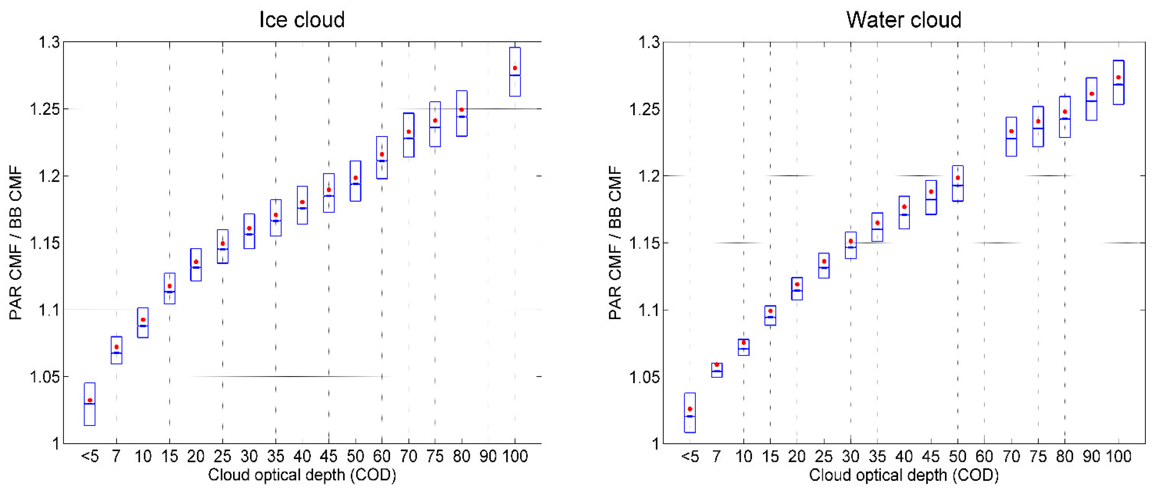
  • The higher the cloud thickness, the less precise APOLLO. The expression that derived the PAR CMF as a function of the BB CMF, COD, and cloud type also combined the uncertainties of the subjacent models. Therefore, another alternative should be to explore an expression that avoids dependence on the COD but pays more attention to the type of weather, such as PAR CMF = a × BB CMF + b, where a and b would depend on the type of cloud (water/ice) and the type of weather: overcast skies, broken cloud conditions, and close to clear-sky conditions.

7. Conclusions and Policy Recommendations

This study assessed the performance of 11 methods for estimating surface PAR from satellite imagery in all-sky conditions at 33 ground-based stations. The set of 33 ground-based stations resulted from a careful inspection of the quality of a larger set of 47 ground-based stations located in the MSG prime field of view, from which only reliable measurements were retained.
The relative uncertainty of good-quality measurements is likely to be less stringent for PAR than GHI, for which the targeted uncertainty from Baseline Surface Radiation Network measurements is 2% [64] due to the need for highly accurate solar energy generation estimates. In all-weather or overcast conditions, M1, M4, and M6 met this requirement and should be preferred in Europe, Congo, French Guyana, and South Africa. For other areas, M2, M5, M7, M9, M10, and M11 are good options. M2 and M5 were the best candidates in cloud-free conditions for most sites. M3 and M8 overestimated the PAR levels for most sites and should only be considered when SSIs underestimate radiation. The performance of the HC3- and CAMS-Rad-based methods depended on the geographical location. This observation was less the case for SARAH-3, with a more stable performance across sites, except for Central Africa.
Group 1 methods that compute PAR by multiplying the GHI by a constant coefficient offer an excellent compromise in terms of accuracy, ease of implementation, and capacity to be deployed in real time. Moreover, PAR estimates are immediately available as soon as a GHI estimate is available around the world. Our analysis demonstrated that an optimal coefficient should depend on both the geographical area and the type of sky.
Group 2 methods that rely on a more accurate modeling of the cloud-free and cloudy state of the atmosphere in the PAR spectral range provide pioneering opportunities for research and development. However, they rely on several different resources with both individual and combined levels of uncertainty. In particular, the spectral extinction of clouds as explored in this paper is well-suited for low COD values, but still needs some refinements for higher COD values. As errors accumulate, a simpler function of the PAR CMF based only on the BB CMF, type of cloud, and type of sky might be a promising method to explore. However, despite these advantages, group 2 methods are computationally expensive in terms of both CPU time and memory allocation. In sum, while group 2 methods aim at the better characterization of the atmospheric effects impacting the estimation of PAR, they do not at the moment appear to offer significant benefits over the simpler, less computationally expensive group one methods, though this may change with further research and development.

Supplementary Materials

The following supporting information can be downloaded at: https://www.mdpi.com/article/10.3390/atmos14081259/s1, Figure S1: Validation results for group “Western Europe” combining 7 stations for each method. (a) MBE (%); (b) STDEV (%); (c) RMSE (%); (d) CC. The 3 colors depict the SSIs with which the methods were computed: HC3 in purple, CAMS-Rad in turquoise, and SARAH-3 in khaki. Methods were M1: Jacovides from HC3; M2: Udo et Aro from HC3; M3: Szeicz from HC3; M4: Weighted_Kato with BB CMF from HC3; M5: Weighted_Kato with PAR CMF from HC3; M6: Jacovides from CAMS-Rad; M7: Udo et Aro from CAMS-Rad; M8: Szeicz from CAMS-Rad; M9: Weighted_Kato with BB CMF from CAMS-Rad; M10: Weighted_Kato with PAR CMF from CAMS-Rad; and M11: DWD SARAH-3, Figure S2: Same as Figure S1, but for group “Central Europe”, Figure S3: Same as Figure S1, but for group “Mediterranean”, Figure S4: Same as Figure S1, but for group “Eastern Europe”, Figure S5: Same as Figure S1, but for group “Central Spain”, Figure S6: Same as Figure S1, but for group “Congo”, Figure S7: Same as Figure S1, but for group “Moldova”, Figure S8: Same as Figure S1, but for group “Israel”, Figure S9: Same as Figure S1, but for group “French Guyana”, Figure S10: Same as Figure S1, but for group “Uruguay”, Figure S11: Same as Figure S1, but for group “South Africa”, Figure S12: Same as Figure S1, but for group “Senegal”, Figure S13: Map of k-means clustering with k = 12 based on the variables precipitation, temperature, downward shortwave radiation, enhanced vegetation index, and fraction of absorbed photosynthetically active radiation (Zscheischler et al. [58]), Figure S14: Map with the podiums of method performance per group, Figure S15: Map with the optimal coefficients to estimate PAR from GHI per group in the geographical coverage of MSG prime, Table S1: Validation results for the comparison between the 11 methods to estimate PAR from satellite imagery at the 33 in situ stations in all-weather conditions, Table S2: Validation results for the comparison between the 11 methods to estimate PAR from satellite imagery at the 33 in situ stations in cloud-free conditions (PAR CMF > 0.8), Table S3: Validation results for the comparison between the 11 methods to estimate PAR from satellite imagery at the 33 in situ stations in overcast conditions (PAR CMF < 0.3).

Author Contributions

C.T. oversaw the collection of the in situ measurements, exchanges with all data providers, interaction with DWD to receive and adapt SARAH-3 datasets to support the research approach, the generation of all PAR time series estimated from satellite imagery, the validation of model performance at all sites except the site in Uruguay, and the writing of the paper and production of most of the figures. W.W.N. challenged the assumption that clouds are spectrally neutral under the supervision of A.A. (Antti Arola). He developed a spectral version of cloud extinction. He also regularly interacted and provided relevant feedback to Claire in her task of validating the satellite PAR methods. He was the author of the description of associated methods M5 and M10. U.P. and J.T. provided the SARAH-3 time series at all ground sites. They wrote the text describing the model and reviewed the whole paper before submission. S.D. sourced several in situ UK datasets: Aberystwyth University and Abbotts Hall. With his extensive and relevant experience in both research and industry in the PAR domain, S.D. wrote major elements of the framework and state-of-the-art approaches in this paper as well as optimizing the English language. A.L. carried out the quality assessment of the methods at the site in Uruguay. C.T. and A.L. also had an earlier opportunity to work together on similar evaluation activities regarding the performance of alternative satellite methods for the assessment of ultra-violet radiation. It is obvious that this collaboration contributed to the development of combined expertise with respect to spectral radiation assessment. M.F. provided all the high-quality datasets from the Czech Republic. With numerous discussions and exchanges of experience in the last few years, Milan actively contributed to this effort by providing an alternative and complementary vision of this quality assessment work. Last but not least, A.A. (Alexandr Aculinin) supplied the very long-term and excellent-quality dataset at Kishinev, Moldova. His extensive experience and great generosity contributed relevance and coherence to this work. All authors have read and agreed to the published version of the manuscript.

Funding

The research leading to these results received partial funding from the Framework Partnership Agreement on Copernicus User Uptake of the European Union through the French Spatial Agency CNES: Action 2019-3-15; Consult.: ORADAJARSB-2020-10141480; STS: DIA/CD-2020.0034255.

Data Availability Statement

Ground measurements are the unique property of the data providers. Most datasets are consequently accessible on demand for research purposes. Contact names are available in the acknowledgments section below. PAR datasets derived from satellite imagery are available on demand by contacting William Wandji Nyamsi. SARAH-3 data are freely available from CM SAF, www.cmsaf.eu, e.g., via the doi webpage, https://doi.org/10.5676/EUM_SAF_CM/SARAH/V003 accessed on 1 June 2023. The EFDC datasets can be accessed using the portal, which was in operation in January 2023: http://www.europe-fluxdata.eu/ accessed on 1 June 2023. Select the item “Data” in the top menu, then “Request data”. Registration is required to be able to access and download the datasets.

Acknowledgments

The authors are grateful to all in situ measurement providers for the supply of their measurements, and to: (1) Jon Paul McCalmont from the Institute of Biological, Environmental and Rural Science (IBERS), UK, for the supply of the measurements at Aberystwyth University; (2) Tim Hill and Melanie Chocholek from the Coastal Biodiversity and Ecosystem Service Sustainability (CBESS) institute, NERC Environmental Information Data Center, UK, for the measurements collected at Abbotts Hall; (3) Valenzuela Balderrama, Rita Ximena, and her partners from CIEMAT, Spain, for the provision of the measurements at the Spanish stations (we would also like to thank Rita’s partners at each site—ITAP for the site of Albacete, IFAPA for Cordoba, USC for Lugo, CIALE for Salamanca, SERIDA for Villaviciosa (Asturias), NEIKER for Vitoria-Gasteiz (Alava), and AULA DEI CSIC for Zaragoza); (4) Nathalie Philippon-Blanc and Armand Mariscal, CNRS, Grenoble, France, for the datasets at Bambidie, Pokola, and Mokabi (we are also grateful to the projects FFEM “DynAfFor” and ANR/DFG “DYVALOCCA”, which funded the cost and installation of these stations); (5) Kamel Soudani from the University of Paris Saclay, France, for the Fontainebleau dataset; (6) Frédéric Bornet, INRA, France, for the data from the Péronne Saint-Quentin site, and for his long-term support; (7) Didier Combes, INRAE, France for the PAR dataset collected on the stadium rooftop of Valenciennes, and for the helpful and informative discussion concerning the PAR data market; and (8) Marian Pavelka from the Global Change Research Institute of the Czech Academy of Sciences for providing the data from the in situ network in the Czech Republic and ensuring the high standards of long-term data collection. We are also grateful to the project SustES—“Adaptation strategies for sustainable ecosystem services and food security under adverse environmental conditions” (CZ.02.1.01/0.0/0.0/16_019/0000797). We are grateful to the Copernicus Atmosphere Monitoring Service (CAMS) of the European Union for making available the CAMS McClear and CAMS-Rad datasets. We also thank Marion Schroedter-Homestead from DLR, Germany, for providing high-quality APOLLO cloud properties.

Conflicts of Interest

The authors declare no conflict of interest.

Acronyms

AcronymMeaning
APOLLO NGAVHRR Processing Scheme over Clouds, Land, and Oceans—New Generation
BBBroadband
BB CMFBB cloud modification factor
CAMSCopernicus Atmosphere Monitoring Service
CAMS-RadCAMS Radiation Service
CCCorrelation coefficient
CIEMATCentro de Investigaciones Energéticas, Medioambientales y Tecnológicas
CM SAFSatellite Application Facility on Climate Monitoring
CODCloud optical depth
DALDaylight
DLRGerman Aerospace Center
DWDDeutscher WetterDienst
EFDCEuropean Fluxes Database Cluster
EUMETSATEuropean Organization for the Exploitation of Meteorological Satellites
FMIFinnish Meteorological Institute
GHIGlobal horizontal irradiation
HC3HelioClim-3
K c B B Cloud extinction in the broadband range ( K c B B = GHI/GHI in cloud-free conditions)
K c P A R Cloud extinction in the PAR range ( K c P A R = PAR/PAR in cloud-free conditions)
MBEMean bias error
PARPhotosynthetically active radiation
PAR CMFPAR cloud modification factor
PPFDPhotosynthetic photon flux density
RMSERoot mean square error
RTMRadiative transfer model
SRTMShuttle Radar Topography Mission
SSISurface solar irradiance (or irradiation)
ToATop of atmosphere
STDStandard deviation

References

  1. McCree, K.J. Photosynthetically active radiation. In Physiology Plant Ecology I; Springer: Berlin/Heidelberg, Germany, 1981; pp. 41–55. [Google Scholar]
  2. Frolking, S.E.; Bubier, J.L.; Moore, T.R.; Ball, T.; Bellisario, L.M.; Bhardwaj, A.; Carroll, P.; Crill, P.M.; Lafleur, P.M.; McCaughey, J.H.; et al. Relationship between ecosystem productivity and photosynthetically active radiation for northern peatlands. Glob. Biogeochem. Cycles 1998, 12, 115–126. [Google Scholar] [CrossRef] [Green Version]
  3. Frouin, R.; Murakami, H. Estimating photosynthetically available radiation at the ocean surface from ADEOS-II global imager data. J. Oceanogr. 2007, 63, 493–503. [Google Scholar] [CrossRef]
  4. Larcher, W. Physiological Plant Ecology: Ecophysiology and Stress Physiology of Functional Groups; Springer Science & Business Media: Berlin/Heidelberg, Germany, 2003. [Google Scholar]
  5. Running, S.W.; Nemani, R.R.; Heinsch, F.A.; Zhao, M.; Reeves, M.; Hashimoto, H. A Continuous Satellite-Derived Measure of Global Terrestrial Primary Production. Bioscience 2004, 54, 547–560. [Google Scholar] [CrossRef] [PubMed] [Green Version]
  6. Twitchen, C.; Else, M.A.; Hadley, P. The effect of temperature and light intensity on rate of strawberry fruit ripening. Acta Hortic. 2021, 1309, 643–648. [Google Scholar] [CrossRef]
  7. The Forsyth Barr Stadium—the World’s First Permanently-Roofed Stadium with Natural Turf. Available online: https://www.pitchcare.com/news-media/the-forsyth-barr-stadium-the-worlds-first-permanently-roofed-stadium-with-natural-turf.html (accessed on 1 March 2023).
  8. Hwang, D.J.; Frouin, R.; Tan, J.; Ahn, J.-H.; Choi, J.-K.; Moon, J.-E.; Ryu, J.-H. Algorithm to estimate daily PAR at the ocean surface from GOCI data: Description and evaluation. Front. Mar. Sci. 2022, 9, 924967. [Google Scholar] [CrossRef]
  9. Zhang, X.; Zhang, Y.; Zhoub, Y. Measuring and modelling photosynthetically active radiation in Tibet Plateau during April–October. Agric. For. Meteorol. 2000, 102, 207–212. [Google Scholar] [CrossRef]
  10. Gonzalez, J.A.; Calbo, J. Modelled and measured ratio of PAR to global radiation under cloudless skies. Agric. For. Meteorol. 2002, 110, 319–325. [Google Scholar] [CrossRef]
  11. Jacovides, C.P.; Timvios, F.S.; Papaioannou, G.; Asimakopoulos, D.N.; Theofilou, C.M. Ratio of PAR to broadband solar radiation measured in Cyprus. Agric. For. Meteorol. 2004, 121, 135–140. [Google Scholar] [CrossRef]
  12. Udo, S.O.; Aro, T.O. Global PAR related to global solar radiation for central Nigeria. Agric. For. Meteorol. 1999, 97, 21–31. [Google Scholar] [CrossRef]
  13. Nwokolo, S.C.; Proutsos, N.; Meyer, E.L.; Ahia, C.C. Machine Learning and Physics-Based Hybridization Models for Evaluation of the Effects of Climate Change and Urban Expansion on Photosynthetically Active Radiation. Atmosphere 2023, 14, 687. [Google Scholar] [CrossRef]
  14. Nwokolo, S.C.; Ogbulezie, J.C.; Obiwulu, A.U. Impacts of Climate Change and Meteo-Solar Parameters on Photosynthetically Active Radiation Prediction Using Hybrid Machine Learning with Physics-Based Models. Adv. Space Res. 2022, 70, 3614–3637. [Google Scholar] [CrossRef]
  15. Boilley, A.; Wald, L. Comparison between meteorological re-analyses from ERA-Interim and MERRA and measurements of daily solar irradiation at surface. Renew. Energy 2015, 75, 135–143. [Google Scholar] [CrossRef]
  16. Gelaro, R.; McCarty, W.; Suárez, M.J.; Todling, R.; Molod, A.; Takacs, L.; Randles, C.; Darmenov, A.; Bosilovich, M.G.; Reichle, R.; et al. The Modern-Era Retrospective Analysis for Research and Applications, Version 2 (MERRA-2). J. Clim. 2017, 30, 5419–5454. [Google Scholar] [CrossRef] [PubMed]
  17. Jones, P.D.; Harpham, C.; Troccoli, A.; Gschwind, B.; Ranchin, T.; Wald, L.; Goodess, C.M.; Dorling, S. Using ERA-Interim reanalysis for creating datasets of energy-relevant climate variables. Earth Syst. Sci. Data 2017, 9, 471–495. [Google Scholar] [CrossRef] [Green Version]
  18. Bengulescu, M.; Blanc, P.; Boilley, A.; Wald, L. Do modelled or satellite-based estimates of surface solar irradiance accurately describe its temporal variability? Adv. Sci. Res. 2017, 14, 35–48. [Google Scholar] [CrossRef]
  19. Trolliet, M.; Walawender, J.P.; Bourlès, B.; Boilley, A.; Trentmann, J.; Blanc, P.; Lefèvre, M.; Wald, L. Downwelling surface solar irradiance in the tropical Atlantic Ocean: A comparison of re-analyses and satellite-derived data sets to PIRATA measurements. Ocean Sci. 2018, 14, 1021–1056. [Google Scholar] [CrossRef] [Green Version]
  20. Albarelo, T.; Marie Joseph, I.; Primerose, A.; Seyler, F.; Linguet, L.; Wald, L. Optimizing the Heliosat-II method for surface solar irradiation estimation with GOES images. Can. J. Remote. Sens. 2015, 41, 86–100. [Google Scholar] [CrossRef]
  21. Amillo, A.G.; Huld, T.; Mueller, R. A New Database of Global and Direct Solar Radiation Using the Eastern Meteosat Satellite. Models Valid. Remote Sens. 2014, 6, 8165–8189. [Google Scholar] [CrossRef] [Green Version]
  22. Blanc, P.; Gschwind, B.; Lefèvre, M.; Wald, L. The HelioClim project: Surface solar irradiance data for climate applications. Remote Sens. 2011, 3, 343–361. [Google Scholar] [CrossRef] [Green Version]
  23. Lefevre, M.; Oumbe, A.; Blanc, P.; Espinar, B.; Gschwind, B.; Qu, Z.; Wald, L.; Schroedter-Homscheidt, M.; Hoyer-Klick, C.; Arola, A.; et al. McClear: A new model estimating downwelling solar radiation at ground level in clear-sky conditions. Atmos. Meas. Tech. 2013, 6, 2403–2418. [Google Scholar] [CrossRef] [Green Version]
  24. Marchand, M.; Saint-Drenan, Y.-M.; Saboret, L.; Wey, E.; Wald, L. Performance of CAMS Radiation Service and HelioClim-3 databases of solar radiation at surface: Evaluating the spatial variation in Germany. Adv. Sci. Res. 2020, 17, 143–152. [Google Scholar] [CrossRef]
  25. Qu, Z.; Gschwind, B.; Lefèvre, M.; Wald, L. Improving HelioClim-3 estimates of surface solar irradiance using the McClear clear-sky model and recent advances in atmosphere composition. Atmos. Meas. Tech. 2014, 7, 3927–3933. [Google Scholar] [CrossRef] [Green Version]
  26. Qu, Z.; Oumbe, A.; Blanc, P.; Espinar, B.; Gesell, G.; Gschwind, B.; Klüser, L.; Lefèvre, M.; Saboret, L.; Schroedter-Homscheidt, M.; et al. Fast radiative transfer parameterisation for assessing the surface solar irradiance: The Heliosat-4 method. Meteorol. Z. 2017, 26, 33–57. [Google Scholar] [CrossRef]
  27. Thomas, C.; Wey, E.; Blanc, P.; Wald, L. Validation of three satellite-derived databases of surface solar radiation using measurements performed at 42 stations in Brazil. Adv. Sci. Res. 2016, 13, 81–86. [Google Scholar] [CrossRef] [Green Version]
  28. Thomas, C.; Saboret, L.; Wey, E.; Blanc, P.; Wald, L. Validation of the new HelioClim-3 version 4 real-time and short-term forecast service using 14 BSRN stations. Adv. Sci. Res. 2016, 13, 129–136. [Google Scholar] [CrossRef] [Green Version]
  29. Tournadre, B. Heliosat-V: Une méthode polyvalente d’estimation du rayonnement solaire au sol par satellite. Ph.D. Thesis, Université Paris Sciences et Lettres, Paris, France, 2020. [Google Scholar]
  30. Xie, Y.; Sengupta, M.; Dudhia, J. A Fast All-sky Radiation Model for Solar applications (FARMS): Algorithm and performance evaluation. Sol. Energy 2016, 135, 435–445. [Google Scholar] [CrossRef]
  31. Wandji Nyamsi, W.; Saint-Drenan, Y.-M.; Arola, A.; Wald, L. Further validation of the estimates of the downwelling solar radiation at ground level in cloud-free conditions provided by the McClear service: The case of Sub-Saharan Africa and the Maldives Archipelago. Atmos. Meas. Tech. 2023, 16, 2001–2036. [Google Scholar] [CrossRef]
  32. Thomas, C.; Dorling, S.; Wandji Nyamsi, W.; Wald, L.; Rubino, S.; Saboret, L.; Trolliet, M.; Wey, E. Assessment of five different methods for the estimation of surface photosynthetically active radiation from satellite imagery at three sites—Application to the monitoring of indoor soft fruit crops in southern UK. Adv. Sci. Res. 2019, 16, 229–240. [Google Scholar] [CrossRef] [Green Version]
  33. Light Measurement. Available online: https://www.licor.com/documents/3bjwy50xsb49jqof0wz4 (accessed on 1 March 2023).
  34. Augustine, J.A.; Deluisi, J.J.; Long, C.N. SURFRAD—A national surface radiation budget network for atmospheric research. Bull. Am. Meteorol. Soc. 2020, 81, 2341–2357. [Google Scholar] [CrossRef]
  35. McCree, K.J. Test of current definitions of photosynthetically active radiation against leaf photosynthesis data. Agric. Forest. Meteorol. 1972, 10, 443–453. [Google Scholar] [CrossRef]
  36. Peel, M.C.; Finlayson, B.L.; McMahon, T.A. Updated world map of the Köppen-Geiger climate classification. Hydrol. Earth Syst. Sci. 2007, 11, 1633–1644. [Google Scholar] [CrossRef] [Green Version]
  37. Beck, H.E.; Zimmermann, N.E.; McVicar, T.R.; Vergopolan, N.; Berg, A.; Wood, E.F. Present and future Köppen-Geiger climate classification maps at 1-km resolution. Sci. Data 2018, 5, 180214. [Google Scholar] [CrossRef] [PubMed] [Green Version]
  38. Opálková, M.; Navrátil, M.; Špunda, V.; Blanc, P.; Wald, L. A database of 10 min average measurements of solar radiation and meteorological variables in Ostrava, Czech Republic. Earth Syst. Sci. Data 2018, 10, 837–846. [Google Scholar] [CrossRef] [Green Version]
  39. Korany, M.; Boraiy, M.; Eissa, Y.; Aoun, Y.; Abdel Wahab, M.M.; Alfaro, S.C.; Blanc, P.; El-Metwally, M.; Ghedira, H.; Hunger-shoefer, K.; et al. A database of multi-year (2004–2010) quality-assured surface solar hourly irradiation measurements for the Egyptian territory. Earth Syst. Sci. Data 2016, 8, 105–113. [Google Scholar] [CrossRef] [Green Version]
  40. Rigollier, C.; Lefèvre, M.; Wald, L. The method Heliosat-2 for deriving shortwave solar radiation from satellite images. Sol. Energy 2004, 77, 159–169. [Google Scholar] [CrossRef] [Green Version]
  41. Oumbe, A.; Qu, Z.; Blanc, P.; Lefèvre, M.; Wald, L.; Cros, S. Decoupling the effects of clear atmosphere and clouds to simplify calculations of the broadband solar irradiance at ground level. Geosci. Model. Dev. 2014, 7, 1661–1669, Erratum in Geosci. Model. Dev. 2014, 7, 2409. [Google Scholar] [CrossRef] [Green Version]
  42. Pfeifroth, U.; Drücke, J.; Trentmann, J.; Hollmann, R. SARAH-3—A new satellite-based Climate Data Record for surface radiation parameters from the CM SAF. In Proceedings of the EMS Annual Meeting 2021, Online, 6–10 September 2021. EMS2021-454. [Google Scholar] [CrossRef]
  43. Pfeifroth, U.; Kothe, S.; Drücke, J.; Trentmann, J.; Schröder, M.; Selbach, N.; Hollmann, R. Surface Radiation Data Set—Heliosat (SARAH)—Edition 3; Satellite Application Facility on Climate Monitoring: Offenbach am Main, Germany, 2023. [Google Scholar] [CrossRef]
  44. Müller, R.; Pfeifroth, U.; Träger-Chatterjee, C.; Trentmann, J.; Cremer, R. Digging the METEOSAT Treasure—3 Decades of Solar Surface Radiation. Remote Sens. 2015, 7, 8067–8101. [Google Scholar] [CrossRef] [Green Version]
  45. Mueller, R.; Behrendt, T.; Hammer, A.; Kemper, A. A New Algorithm for the Satellite-Based Retrieval of Solar Surface Irradiance in Spectral Bands. Remote Sens. 2012, 4, 622–647. [Google Scholar] [CrossRef] [Green Version]
  46. Szeicz, G. Solar radiation for plant growth. J. Appl. Ecol. 1974, 11, 617–636. [Google Scholar] [CrossRef]
  47. Yu, X.; Wu, Z.; Jiang, W.; Guo, X. Predicting daily photosynthetically active radiation from global solar radiation in the Contiguous United States. Energy Convers. Manag. 2015, 89, 71–82. [Google Scholar] [CrossRef]
  48. Su, W.; Charlock, T.P.; Rose, F.G.; Rutan, D. Photosynthetically active radiation from Clouds and the Earth’s Radiant Energy System (CERES) products. J. Geophys. Res. Biogeosci. 2007, 112, G02022. [Google Scholar] [CrossRef] [Green Version]
  49. Zhang, H.; Dong, X.; Xi, B.; Xin, X.; Liu, Q.; He, H.; Xie, X.; Li, L.; Yu, S. Retrieving high-resolution surface photosynthetically active radiation from the MODIS and GOES-16 ABI data. Remote Sens. Environ. 2021, 260, 112436. [Google Scholar] [CrossRef]
  50. Tang, W.; Qin, J.; Yang, K.; Jiang, Y.; Pan, W. Mapping long-term and high-resolution global gridded photosynthetically active radiation using the ISCCP H-series cloud product and reanalysis data. Earth Syst. Sci. Data 2022, 14, 2007–2019. [Google Scholar] [CrossRef]
  51. Kato, S.; Ackerman, T.; Mather, J.; Clothiaux, E. The k-distribution method and correlated-k approximation for short-wave radiative transfer model. J. Quant. Spectrosc. Radiat. Transf. 1999, 62, 109–121. [Google Scholar] [CrossRef]
  52. Wandji Nyamsi, W.; Espinar, B.; Blanc, P.; Wald, L. How close to detailed spectral calculations is the k-distribution method and correlated-k approximation of Kato et al. (1999) in each spectral interval? Meteorol. Z. 2014, 23, 547–556. [Google Scholar] [CrossRef] [Green Version]
  53. Wandji Nyamsi, W.; Arola, A.; Blanc, P.; Lindfors, A.V.; Cesnulyte, V.; Pitkänen, M.R.A.; Wald, L. Technical Note: A novel parameterization of the transmissivity due to ozone absorption in the k-distribution method and correlated-k approximation of Kato et al. (1999) over the UV band. Atmos. Chem. Phys. 2015, 15, 7449–7456. [Google Scholar] [CrossRef] [Green Version]
  54. Wandji Nyamsi, W.; Espinar, B.; Blanc, P.; Wald, L. Estimating the photosynthetically active radiation under clear skies by means of a new approach. Adv. Sci. Res. 2015, 12, 5–10. [Google Scholar] [CrossRef] [Green Version]
  55. Wandji Nyamsi, W.; Pitkänen, M.; Aoun, Y.; Blanc, P.; Heikkilä, A.; Lakkala, K.; Bernhard, G.; Koskela, T.; Lindfors, A.; Arola, A.; et al. A new method for estimating UV fluxes at ground level in cloud-free conditions. Atmos. Meas. Tech. 2017, 10, 4965–4978. [Google Scholar] [CrossRef] [Green Version]
  56. Wandji Nyamsi, W.; Blanc, P.; Augustine, J.A.; Arola, A.; Wald, L. A new clear-sky method for assessing photosynthetically active radiation at the surface level. Atmosphere 2019, 10, 219. [Google Scholar] [CrossRef] [Green Version]
  57. Wandji Nyamsi, W.; Blanc, P.; Dumortier, D.; Mouangue, R.; Arola, A.; Wald, L. Using Copernicus Atmosphere Monitoring Service (CAMS) Products to Assess Illuminances at Ground Level under Cloudless Conditions. Atmosphere 2021, 12, 643. [Google Scholar] [CrossRef]
  58. Mayer, B.; Kylling, A. Technical note: The libRadtran software package for radiative transfer calculations-description and examples of use. Atmos. Chem. Phys. 2005, 5, 1855–1877. [Google Scholar] [CrossRef] [Green Version]
  59. Emde, C.; Buras-Schnell, R.; Kylling, A.; Mayer, B.; Gasteiger, J.; Hamann, U.; Kylling, J.; Richter, B.; Pause, C.; Dowling, T.; et al. The libRadtran software package for radiative transfer calculations (version 2.0.1). Geosci. Model. Dev. 2016, 9, 1647–1672. [Google Scholar] [CrossRef] [Green Version]
  60. Gueymard, C.A. The sun’s total and the spectral irradiance for solar energy applications and solar radiations models. Sol. Energy 2004, 76, 423–452. [Google Scholar] [CrossRef]
  61. Marchand, M.; Lefèvre, M.; Saboret, L.; Wey, E.; Wald, L. Verifying the spatial consistency of the CAMS Radiation Service and HelioClim-3 satellite-derived databases of solar radiation using a dense network of measuring stations: The case of the Netherlands. Adv. Sci. Res. 2019, 16, 103–111. [Google Scholar] [CrossRef] [Green Version]
  62. Zscheischler, J.; Miguel, D.M.; Harmeling, S. Climate classifications: The value of unsupervised clustering. Procedia Comput. Sci. 2012, 9, 897–906. [Google Scholar] [CrossRef] [Green Version]
  63. Aculinin, A. Photosynthetically active radiation in Moldova. Mold. J. Phys. Sci. 2008, 7, 115–123. [Google Scholar]
  64. Ohmura, A.; Gilgen, H.; Hegner, H.; Mueller, G.; Wild, M.; Dutton, E.G.; Forgan, B.; Froelich, C.; Philipona, R.; Heimo, A.; et al. Baseline Surface Radiation Network (BSRN/WCRP): New precision radiometry for climate research. Bull. Am. Meteorol. Soc. 1998, 79, 2115–2136. [Google Scholar] [CrossRef]
Figure 1. Geographical distribution of surface in situ PAR stations, with the Köppen–Geiger climate classification as the background [37] and the number of PAR stations falling into each class (between brackets in the legend).
Atmosphere 14 01259 g001
Figure 2. Simulation results of the ratio of PAR CMF to BB CMF for ice clouds (left) and water clouds (right) as function of cloud optical depth. The mean values of the boxes are marked with a red dot. The 1st, 2nd, and 3rd quartiles are marked with a blue line.
Atmosphere 14 01259 g002
Figure 3. Statistical results averaged across the 33 stations for each method, M1–M11. (a) Relative MBE (%); (b) relative STDEV (%); (c) relative RMSE (%); (d) CC. The 3 colors depict the SSIs with which the methods were computed: HC3 in purple, CAMS-Rad in turquoise, and SARAH-3 in khaki. Methods were M1: Jacovides from HC3; M2: Udo et Aro from HC3; M3: Szeicz from HC3; M4: Weighted_Kato with BB CMF from HC3; M5: Weighted_Kato with PAR CMF from HC3; M6: Jacovides from CAMS-Rad; M7: Udo et Aro from CAMS-Rad; M8: Szeicz from CAMS-Rad; M9: Weighted_Kato with BB CMF from CAMS-Rad; M10: Weighted_Kato with PAR CMF from CAMS-Rad; and M11: SARAH-3.
Atmosphere 14 01259 g003
Table 1. Thirty-three in situ surface PAR measurement stations and associated meta-information. Color indicates Köppen–Geiger climate type, with green for temperate climate without dry season and warm summer (Cfb), light brown for arid and cold climate of steppe type (Bsk), yellow for temperate climate with dry and hot summer (Csa), deep sky blue for cold climate without dry season and with warm summer (Dfb), yellow-green for temperate climate with dry and warm summer (Csb), blue for tropical climate of monsoon type (Am), orange for arid and hot climate of steppe type (Bsh), pale green for temperate climate with dry winter and hot summer (Cwa), and green-yellow for temperate climate without dry season and with hot summer (Cfa).
33 StationsStation Details and CountryContacts and ProjectsClimate from Köppen-Geiger ClassificationLatitude (°)Longitude (°)Height (m)Start DateEnd DateTime Step (min)Time Reference (UT+hours)Begin/Middle/End of Interval Hypothesis (NR: Not Relevant)
Aberystwyth UniversityUnited Kingdom (UK)Jon Paul McCalmont, IBERS Cfb52.422−4.0701101 January 201231 December 2017300middle
Abbotts HallUKTim Hill and Melanie Chocholek, CBESSCfb51.78580.8669215 December 201227 January 2015300middle
AlbaceteSpain (SP)Rita Valenzuela, CIEMATBSk39.04−2.086981 June 201931 December 202110NR
CordobaSP Rita Valenzuela, CIEMATCsa37.86−4.80911 June 201931 December 202010NR
Czech_BKF_SFBily Kriz Forest, spruce forest after thinning, Czech Republic (CR)Milan Fischer, Global Change Research Institute GCASDfb49.502118.536988423 April 200831 December 2020101end
Czech_BKF_STBily Kriz Forest, meteorological station (CR)Milan Fischer, GCASDfb49.502618.53868901 January 200831 December 2020101end
Czech_BKGBily Kriz Grassland (CR)Milan Fischer, GCASDfb49.494418.54298661 January 200831 December 2020101end
Czech_KRPKresin agroecosystem (CR)Milan Fischer, GCASDfb49.573215.07875401 January 201331 December 2020101end
Czech_LNZLandzhot, wetland forest (CR)Milan Fischer, GCASDfb48.681516.946317229 August 201431 December 2020101end
Czech_RAJRajec, spure forest (CR)Milan Fischer, GCASDfb49.443716.69656511 June 201131 December 2020101end
Czech_STIStitna, Beech forest (CR)Milan Fischer, GCAS Dfb49.03617.969955111 March 200931 December 2020101end
Czech_TRE Trebon, Wetland (CR)Milan Fischer, GCASDfb49.024714.770342529 April 200631 December 2020301end
EFDC_DE-HaiHainich, Germany (DE) European Fluxes Database Cluster (EFDC) interface, project CarboExtreme, ICOSDfb51.079410.45214601 February 200431 December 2020301end
EDFC_FR-AurAurade, France (FR)EFDC, CarboEuropeIP, GHG-Europe, Integrated Carbon Observation System (ICOS) station—Tiphaine Tallec and Aurore Brut, CESBIOCfb43.54961.106124231 January 200430 August 2021301end
EFDC_FR-PuePuechabon (FR)EFDC, CarboEuropeIP, CarboEuroFlux, Medeflu, IMECC GHG-Europe, ICOS station, CarboExtremeCsb43.74133.59572761 February 200431 December 2018301end
EFDC_GF-GuyGuyaflux (FR)EFDC, ICOS stationAm5.27878−52.9249371 February 20041 January 201630−3end
EFDC_IE-DriDripsey, Ireland (IE)EFDC, CarboEuropeIPCfb51.9867−8.75181881 February 200431 December 2013300end
EFDC_IL-YatEFDC, Yatir, Israel (IL)EFDC, CarboEuropeIP, CarboEuroFluxCsa31.34535.0526541 February 200431 December 2018302end
EFDC_IT-BCiBorgo Cioffi, Italy (IT)EFDC, CarboEuropeIP, CarboItaly, ICOS stationCsa40.523814.957471 February 200431 December 2019301end
EFDC_IT-NoeArca di Noe, Le Prigionette (IT)EFDC, CarboEuropeIP, CarboItaly, Medeflu, CarboExtreme, ICOS stationCsa40.60628.1517261 February 200431 December 2008301end
EFDC_RU-FyoFyodorovskoye, Russia (RU)EFDC, GHG-Europe, InGOS, TCOS-SiberiaDfb56.461532.92212731 February 200431 December 2020303end
EFDC_SN-DhrDahra, Senegal (SN)EFDC, CarboAfrica, GHG-EuropeBsh15.4028−15.4322431 January 201031 December 2013300end
EFDC_UK_AMoAuchencorth Moss (UK)EFDC, CarboEuropeIP, CarboExtreme, ICOS stationCfb55.7925−3.243622641 February 200431 December 2016300end
EFDC_ZA-KruSkukuza, South Africa (ZA)EFDC, CarboAfrica Cwa−25.019731.496936531 December 200831 December 2010302end
KishinevMoldovaAlexandr Aculinin, Institute of Applied Physics (IAP) Dfb47.001428.81562051 January 200431 May 202110NR
LugoSPRita Valenzuela, CIEMATCsb43.00−7.544471 June 201931 December 202010NR
Peronne Saint-QuentinFRFrédéric Bornet, INRACfb49.87213.02078421 November 201306 August 2021300end
PokolaCongoN. Philippon-Blanc and A. Mariscal, CNRSAm1.403616.31673322 January 201928 November 2021150begin
UruguayUruguayAgustin Laguarda, Univ. de la RepúblicaCfa−31.282−57.918561 January 201731 December 202010end
ValenciennesRooftop of the Valenciennes football stadium, FRDidier Combes, INRAECfb50.34873.53153722 February 201931 December 201910NR
Villaviciosa (Asturias)SPRita Valenzuela, CIEMATCfb43.48−5.4461 June 201931 December 202010NR
Vitoria-Gasteiz (Alava)SP Rita Valenzuela, CIEMAT Cfb42.85−2.625201 June 201931 December 202010NR
ZaragozaSPRita Valenzuela, CIEMAT BSk41.73−0.812261 June 201931 December 202010NR
Table 2. The initial number of PAR records (column 2), the percentage of records discarded by the quality check (column 3), and the resulting final number of records available (column 4) at the original timestep of each of the 33 retained in situ measurement stations.
StationsNb Total Slots (at the Original Time Step of the Station)Total Percentage of Discarded ValuesFinal Number of Slots
Aberystwyth University49,8821%49,614
Abbotts Hall15,3450%15,345
Albacete407,0346%382,173
Cordoba407,6471%403,138
Czech_BKF_SF312,6408%287,747
Czech_BKF_ST329,1153%318,431
Czech_BKG311,52012%275,339
Czech_KRP203,4360%203,380
Czech_LNZ159,9430%159,904
Czech_RAJ243,2864%233,733
Czech_STI297,3500%297,153
Czech_TRE 123,9541%123,266
EFDC_DE-Hai139,88514%120,216
EDFC_FR-Aur134,5671%133,589
EFDC_FR-Pue116,3881%114,740
EFDC_GF-Guy66,7381%66,309
EFDC_IE-Dri68,58826%50,639
EFDC_IL-Yat113,7520%113,364
EFDC_IT-BCi85,80611%77,301
EFDC_IT-Noe39,2110%39,045
EFDC_RU-Fyo135,5801%134,367
EFDC_SN-Dhr26,3200%26,261
EFDC_UK_AMo107,9341%106,991
EFDC_ZA-Kru940148%4833
Kishinev4,356,3350%4,348,111
Lugo407,17812%356,332
Péronne Saint-Quentin60,4820%60,397
Pokola48,9997%45,633
Uruguay28,3490%28,349
Valenciennes210,2402%206,499
Villaviciosa 405,9302%396,216
Vitoria407,1927%397,643
Zaragoza407,3059%372,324
Table 3. Methods (MX) used to estimate PAR from satellite imagery evaluated in this paper and their groups. Group 1 methods define models that apply a constant coefficient directly to the GHI component. Group 2 methods provide a more accurate description of the radiation content in cloud-free conditions according to specific spectral bands (the Kato bands), which are then multiplied by a BB or PAR CMF.
Method IndexMethod NameGroup Number
M1Jacovides from HC31
M2Udo and Aro from HC31
M3Szeicz from HC31
M4Weighted_Kato with BB CMF from HC32
M5Weighted_Kato with PAR CMF from HC32
M6Jacovides from CAMS-Rad1
M7Udo and Aro from CAMS-Rad1
M8Szeicz from CAMS-Rad1
M9Weighted_Kato with BB CMF from CAMS-Rad2
M10Weighted_Kato with PAR CMF from CAMS-Rad2
M11SARAH-32
Table 4. Statistical distributions of values taken by the cosine of the solar zenith angle (SZA), the ground albedo, and the 7 variables describing the clear atmosphere.
VariableValue
SZAUniform between 0 and 89 (degrees)
Ground albedoUniform between 0 and 0.9
Elevation of the ground above mean sea levelEquiprobable in the set {0, 1, 2, 3} (km)
Total column ozoneOzone content is 300 × β + 200 in Dobson units Beta distribution, with A parameter = 2, and B parameter = 2, to compute β
Atmospheric profiles (Air Force Geophysics Laboratory standards)Equiprobable in the set {“Midlatitude Summer”, “Midlatitude Winter”, “Subarctic Summer”, “Subarctic Winter”, “Tropical”, “US. Standard”}
Aerosol optical depth at 550 nmGamma distribution, with shape parameter = 2 and scale parameter = 0.13
Angstrom exponent coefficient Normal distribution, with mean = 1.3 and standard deviation = 0.5
Aerosol typeEquiprobable in the set {“urban”, “rural”, “maritime”, “tropospheric”, “desert”, “continental”, “Antarctic”}
Table 5. Cloud properties.
Cloud Optical DepthWater Cloud (Cloud Base Height + Thickness, km)Ice Cloud (Cloud Base Height + Thickness, km)
0.5, 1, 2, 3 (and 4 for ice cloud only)Cu: 0.4 + 0.2, 1 + 1.6, 1.2 + 0.2, 2 + 0.5
Ac: 2 + 3, 3.5 + 1.5, 4.5 + 1
Ci: 6 + 0.5, 8 + 0.3, 10 + 1
5, 7, 10, 20 (and 15 for ice cloud only)Sc: 0.5 + 0.5, 1.5 + 0.6, 2 + 1, 2.5 + 2
As: 2 + 3, 3.5 + 2, 4.5 + 1
Cs: 6 + 0.5, 8 + 2, 10 + 1
40, 70St: 0.2 + 0.5, 0.5 + 0.3, 1 + 0.5
Ns: 0.8 + 3, 1 + 1
Cb: 1 + 6, 2 + 8
-
Table 6. Values for a0, a1, a2, and a3 parameters for APOLLO cloud optical depths below and above 100.
COD ≤ 100COD > 100
Water CloudsIce CloudsWater Clouds Ice Clouds
a00.0105950620.01595150480.14166788400.1286531944
a10.0062687970.00731677300.00119511320.0015225904
a2−0.00007277−0.0000994434−0.000001971−0.000002432
a30.0000003370.00000051070.00000000140.00000000167
Table 7. PAR station groups and climate classification. Color code is equivalent to Table 1.
Group of StationsNumber of Stations in the GroupStationsKöppen–Geiger Climate Code
“Western Europe” Group7Aberystwyth University
Abbotts Hall
EFDC_FR-Aur
EFDC_IE-Dri
Péronne Saint-Quentin
Valenciennes
Villaviciosa
Cfb
“Central Europe” Group6Czech_KRP
Czech_LNZ
Czech_RAJ
Czech_STI
Czech_TRE
EFDC_DE-Hai
Dfb
“Mediterranean” Group5AlbaceteBsk
Cordoba
EFDC_IT-Bci
EFDC_IT-Noe
Csa
EFDC_FR-PueCsb
“Eastern Europe” Group4Czech_BKF_SF
Czech_BKF_ST
Czech_BKG
EFDC_RU-Fyo
Dfb
“Central Spain” Group3LugoCsb
VitoriaCfb
ZaragozaBsk
“Congo” Group1PokolaAm
“Moldova” Group1KishinevDfb (close to Dfa and BSk)
“Israel” Group1EFDC_IL-YatCsa
“French Guyana” Group1EFDC_GF-GuyAm
“Uruguay” Group1UruguayCfa
“South-Africa” Group1EFDC_ZA-KruCwa
“Senegal” Group1EFDC_SN-DhrBsh
Table 8. Group representativity expressed as the standard deviation values (column 2) and the range (column 3) computed for each statistical quantity. The first row shows the results for all stations, and the 5 subsequent rows correspond to the first 5 groups comprising more than 1 station.
StationSpread of Values (Standard Deviation for Each Statistical Index)Range (Maximum–Minimum)
All stationsMBE 5.3, STD 6.8, RMSE 6.9, CC 0.02MBE 11.7, STD 14.2, RMSE 14.4, CC 0.04
“Western Europe” GroupMBE 2.5, STD 4.6, RMSE 4.6, CC 0.01MBE 6.5, STD 13.6, RMSE 13.4, CC 0.04
“Central Europe” GroupMBE 1.9, STD 2.3, RMSE 2.4, CC 0.01MBE 6.0, STD 6.4, RMSE 6.6, CC 0.03
“Mediterranean” GroupMBE 1.8, STD 3.7, RMSE 3.7, CC 0.01MBE 4.4, STD 8.8, RMSE 8.9, CC 0.03
“Eastern Europe” GroupMBE 1.9, STD 1.6, RMSE 1.6, CC 0.01MBE 4.2, STD 3.3, RMSE 3.7, CC 0.02
“Central Spain” GroupMBE 2.3, STD 4.7, RMSE 5.0, CC 0.01MBE 4.4, STD 9.3, RMSE 9.9, CC 0.02
Table 9. Statistical results per group and per method. Units: µmol m−2 s−1 and percent. NBDATA: number of 30 min records available in the group. Color indicates the performance level of methods between groups: the best method is shown in green with the lowest MBE absolute value, good methods in light green with the second lowest MBE absolute value, bad methods in light red with the second highest MBE absolute value, and the worst method in red with the highest MBE absolute value for each group.
IndexM1M2M3M4M5M6M7M8M9M10M11
“Western Europe”MBE −15.0 (−2.7%)30.8 (5.5%)89.8 (15.9%)6.1 (1.1%)27.7 (4.9%)−4.3 (−0.8%)42.4 (7.5%)102.6 (18.2%)17.2 (3.1%)40.2 (7.1%)38.2 (6.8%)
NBDATA: 323478STD135.8 (24.1%)136.4 (24.2%)152.2 (27.0%)134.7 (23.9%)137.4 (24.3%)143.7 (25.4%)144.2 (25.5%)159.1 (28.2%)143.2 (25.4%)150.8 (26.7%)156.0 (27.6%)
MEANREF: 564.5RMSE136.7 (24.2%)139.9 (24.8%)176.8 (31.3%)134.8 (23.9%)140.2 (24.8%)143.8 (25.5%)150.3 (26.6%)189.3 (33.5%)144.3 (25.6%)156.0 (27.6%)160.6 (28.4%)
CC0.9630.9630.9630.9630.9610.9580.9580.9580.9580.9530.950
“Central Europe”MBE−2.9 (−0.5%)42.1 (7.8%)100.1 (18.4%)13.9 (2.6%)31.8 (5.9%)15.1 (2.8%)61.6 (11.3%)121.5 (22.4%)32.5 (6.0%)55.3 (10.2%)45.1 (8.3%)
NBDATA: 540960STD147.2 (27.1%)156.9 (28.9%)181.6 (33.4%)150.6 (27.7%)149.3 (27.5%)139.7 (25.7%)145.0 (26.7%)165.1 (30.4%)141.7 (26.1%)147.7 (27.2%)151.0 (27.8%)
MEANREF: 543.0RMSE147.3 (27.1%)162.5 (29.9%)207.3 (38.2%)151.3 (27.9%)152.6 (28.1%)140.5 (25.9%)157.6 (29.0%)205.0 (37.8%)145.4 (26.8%)157.7 (29.0%)157.6 (29.0%)
CC0.9520.9520.9520.9520.9530.9560.9560.9560.9560.9530.950
“Mediterranean”MBE2.6 (0.3%)64.9 (8.7%)145.2 (19.5%)32.9 (4.4%)51.4 (6.9%)3.9 (0.5%)66.4 (8.9%)146.8 (19.7%)34.3 (4.6%)51.8 (6.9%)57.6 (7.7%)
NBDATA: 265039STD141.1 (18.9%)146.7 (19.7%)171.5 (23.0%)143.6 (19.3%)149.3 (20.0%)139.6 (18.7%)147.0 (19.7%)174.1 (23.4%)143.6 (19.3%)149.4 (20.0%)147.4 (19.8%)
MEANREF: 745.2RMSE141.1 (18.9%)160.4 (21.5%)224.7 (30.2%)147.3 (19.8%)157.9 (21.2%)139.6 (18.7%)161.3 (21.6%)227.7 (30.6%)147.6 (19.8%)158.1 (21.2%)158.3 (21.2%)
CC0.9670.9670.9670.9670.9650.9680.9680.9680.9680.9650.966
“Eastern Europe”MBE46.6 (9.7%)90.4 (18.9%)146.8 (30.7%)61.0 (12.7%)82.1 (17.1%)38.0 (8.1%)80.5 (17.1%)135.2 (28.7%)51.7 (11.0%)75.3 (16.0%)52.5 (11.1%)
NBDATA: 425945STD163.6 (34.2%)178.5 (37.3%)206.9 (43.2%)170.9 (35.7%)174.3 (36.4%)158.3 (33.6%)165.6 (35.1%)185.3 (39.3%)162.1 (34.4%)167.9 (35.6%)152.6 (32.4%)
MEANREF: 478.9RMSE170.1 (35.5%)200.1 (41.8%)253.7 (53.0%)181.5 (37.9%)192.7 (40.2%)162.8 (34.5%)184.1 (39.0%)229.3 (48.6%)170.2 (36.1%)184.0 (39.0%)161.4 (34.2%)
CC0.9360.9360.9360.9360.9330.9360.9360.9360.9350.9320.943
“Central Spain”MBE34.9 (5.4%)91.6 (14.2%)164.7 (25.5%)63.9 (9.9%)85.4 (13.2%)42.4 (6.6%)99.8 (15.4%)173.7 (26.9%)71.7 (11.1%)93.5 (14.5%)90.0 (13.9%)
NBDATA: 39864STD173.8 (26.9%)180.9 (28.0%)203.6 (31.5%)176.4 (27.3%)181.4 (28.1%)178.8 (27.7%)186.7 (28.9%)210.1 (32.5%)182.3 (28.2%)190.4 (29.5%)190.4 (29.5%)
MEANREF: 645.9RMSE177.3 (27.4%)202.7 (31.4%)261.9 (40.5%)187.6 (29.0%)200.5 (31.0%)183.8 (28.4%)211.6 (32.8%)272.6 (42.2%)195.9 (30.3%)212.1 (32.8%)210.7 (32.6%)
CC0.9470.9470.9470.9480.9450.9440.9440.9440.9440.9400.939
“Congo”MBE−27.9 (−3.5%)37.1 (4.6%)120.8 (15.0%)40.2 (5.0%)63.6 (7.9%)70.0 (8.7%)143.2 (17.7%)237.4 (29.4%)146.8 (18.2%)171.9 (21.3%)157.9 (19.6%)
NBDATA: 15392STD209.6 (26.0%)211.6 (26.2%)227.3 (28.1%)210.3 (26.0%)210.1 (26.0%)213.5 (26.4%)223.3 (27.6%)248.9 (30.8%)223.2 (27.6%)231.8 (28.7%)235.0 (29.1%)
MEANREF: 807.7RMSE211.5 (26.2%)214.8 (26.6%)257.4 (31.9%)214.1 (26.5%)219.5 (27.2%)224.7 (27.8%)265.2 (32.8%)344.0 (42.6%)267.2 (33.1%)288.6 (35.7%)283.1 (35.1%)
CC0.9340.9340.9340.9350.9360.9320.9320.9320.9330.9280.925
“Moldova”MBE−45.7 (−7.0%)5.2 (0.8%)70.8 (10.8%)−23.5 (−3.6%)−3.5 (−0.5%)−49.4 (−7.5%)1.2 (0.2%)66.4 (10.1%)−27.4 (−4.2%)−7.0 (−1.1%)−5.5 (−0.8%)
NBDATA: 140960STD145.6 (22.2%)145.3 (22.1%)162.0 (24.7%)143.6 (21.9%)144.2 (22.0%)142.5 (21.7%)139.1 (21.2%)152.3 (23.2%)138.9 (21.2%)141.2 (21.5%)137.1 (20.9%)
MEANREF: 656.2RMSE152.6 (23.3%)145.4 (22.2%)176.8 (26.9%)145.5 (22.2%)144.2 (22.0%)150.8 (23.0%)139.1 (21.2%)166.1 (25.3%)141.6 (21.6%)141.4 (21.5%)137.2 (20.9%)
CC0.9650.9650.9650.9650.9650.9670.9670.9670.9670.9660.968
“Israel”MBE−37.2 (−3.9%)38.9 (4.1%)137.0 (14.4%)−11.5 (−1.2%)6.9 (0.7%)−44.2 (−4.6%)31.4 (3.3%)128.8 (13.5%)−18.8 (−2.0%)−0.7 (−0.1%)61.2 (6.4%)
NBDATA: 112699STD116.6 (12.3%)126.6 (13.3%)162.2 (17.1%)118.1 (12.4%)122.2 (12.9%)127.1 (13.4%)132.4 (13.9%)161.7 (17.0%)126.4 (13.3%)125.3 (13.2%)141.5 (14.9%)
MEANREF: 950.5RMSE122.4 (12.9%)132.4 (13.9%)212.3 (22.3%)118.6 (12.5%)122.4 (12.9%)134.5 (14.1%)136.1 (14.3%)206.7 (21.7%)127.8 (13.4%)125.3 (13.2%)154.1 (16.2%)
CC0.9810.9810.9810.9810.9800.9780.9780.9780.9780.9780.973
“French Guyana”MBE1.5 (0.2%)70.1 (8.5%)158.3 (19.3%)85.8 (10.5%)114.5 (14.0%)63.7 (7.8%)137.5 (16.7%)232.5 (28.3%)154.6 (18.8%)187.1 (22.8%)170.5 (20.8%)
NBDATA: 65742STD241.9 (29.5%)262.8 (32.0%)299.4 (36.5%)268.1 (32.7%)272.8 (33.2%)227.3 (27.7%)245.0 (29.8%)278.2 (33.9%)249.0 (30.3%)255.1 (31.1%)296.5 (36.1%)
MEANREF: 820.6RMSE241.9 (29.5%)272.0 (33.1%)338.7 (41.3%)281.5 (34.3%)295.9 (36.1%)236.0 (28.7%)280.9 (34.2%)362.6 (44.1%)293.1 (35.7%)316.4 (38.5%)342.0 (41.6%)
CC0.9110.9110.9110.9100.9090.9180.9180.9180.9180.9150.893
“Uruguay”MBE−75.8 (−7.9%)−2.0 (−0.2%)93.0 (9.7%)−23.6 (−2.5%)8.7 (0.9%)−81.3 (−8.5%)−8.0 (−0.8%)86.5 (9.0%)−29.2 (−3.0%)0.0 (0.0%)−2.8 (−0.3%)
NBDATA: 28349STD184.2 (19.2%)195.3 (20.3%)225.1 (23.4%)191.1 (19.9%)219.0 (22.8%)162.7 (16.9%)165.7 (17.2%)187.8 (19.5%)163.8 (17.0%)177.2 (18.4%)186.4 (19.4%)
MEANREF: 961.2RMSE199.2 (20.7%)195.3 (20.3%)243.6 (25.3%)192.5 (20.0%)219.2 (22.8%)181.9 (18.9%)165.9 (17.3%)206.8 (21.5%)166.4 (17.3%)177.2 (18.4%)186.4 (19.4%)
CC0.9520.9520.9520.9520.9360.9630.9630.9630.9630.9560.954
“South Africa”MBE−22.5 (−2.8%)43.5 (5.3%)128.6 (15.8%)25.0 (3.1%)56.6 (7.0%)16.4 (2.0%)85.7 (10.5%)174.8 (21.5%)66.5 (8.2%)99.0 (12.2%)82.1 (10.1%)
NBDATA: 4833STD143.2 (17.6%)145.2 (17.8%)169.5 (20.8%)143.0 (17.6%)152.6 (18.7%)161.0 (19.8%)169.7 (20.8%)199.6 (24.5%)168.8 (20.7%)183.3 (22.5%)154.3 (18.9%)
MEANREF: 814.4RMSE144.9 (17.8%)151.6 (18.6%)212.8 (26.1%)145.2 (17.8%)162.8 (20.0%)161.8 (19.9%)190.1 (23.3%)265.3 (32.6%)181.4 (22.3%)208.3 (25.6%)174.8 (21.5%)
CC0.9730.9730.9730.9730.9700.9650.9650.9650.9640.9580.971
“Senegal”MBE−113.8 (−11.7%)−42.2 (−4.3%)50.0 (5.1%)−64.2 (−6.6%)−49.4 (−5.1%)7.8 (0.8%)89.5 (9.2%)194.7 (20.0%)65.2 (6.7%)78.4 (8.1%)144.2 (14.8%)
NBDATA: 26234STD158.8 (16.3%)162.3 (16.7%)184.5 (19.0%)160.6 (16.5%)158.4 (16.3%)140.0 (14.4%)157.4 (16.2%)196.6 (20.2%)156.0 (16.0%)161.4 (16.6%)170.7 (17.6%)
MEANREF: 972.5RMSE195.4 (20.1%)167.7 (17.2%)191.2 (19.7%)172.9 (17.8%)166.0 (17.1%)140.3 (14.4%)181.1 (18.6%)276.7 (28.5%)169.1 (17.4%)179.4 (18.4%)223.4 (23.0%)
CC0.9620.9620.9620.9620.9630.9720.9720.9720.9700.9670.967
Disclaimer/Publisher’s Note: The statements, opinions and data contained in all publications are solely those of the individual author(s) and contributor(s) and not of MDPI and/or the editor(s). MDPI and/or the editor(s) disclaim responsibility for any injury to people or property resulting from any ideas, methods, instructions or products referred to in the content.

