Aerosol Properties and Their Influences on Marine Boundary Layer Cloud Condensation Nuclei over the Southern Ocean

Abstract

Five overcast marine stratocumulus cases during the Southern Ocean Clouds Radiation Aerosol Transport Experimental Study (SOCRATES) aircraft field campaign were selected to examine aerosol and cloud condensation nuclei (CCN) properties with cloud influence. The Aitken- and accumulation-mode aerosols contributed approximately 70% and 30% of the total aerosols, respectively. The aerosol properties before and after periods of drizzle were investigated using in situ measurements during one case. Sub-cloud drizzle processes impacted accumulation-mode aerosols and CCN distribution. There was a nearly linear increase in CCN number concentration (N_CCN) with supersaturation (S) during the ‘before drizzle’ period, but this was not true for the ‘after drizzle’ period, particularly when S > 0.4%. Using the hygroscopicity parameter (κ) to quantitatively investigate the chemical cloud-processing mechanisms, we found that higher κ values (>0.4) represent cloud-processing aerosols, while lower κ values (<0.1) represent newly formed aerosols. When the supersaturation is less than the Hoppel minimum (0.22%), cloud processing is dominant, whereas sea-spray aerosols are dominant contributors to CCN activation when S exceeds 0.22% but is less than 0.32%, the effective supersaturation threshold. Sea salt is considered a non-cloud-processing aerosol and is large and hygroscopic enough to form cloud droplets.

1. Introduction

Marine boundary layer (MBL) aerosols and clouds are important for the Earth’s hydrological cycle, radiation budget [1,2], and, ultimately, climate [3,4,5]. Despite their importance, realistically simulating MBL aerosols and clouds in global climate models (GCMs) remains a challenge. Many improvements have been made in phase 6 of the Coupled Model Intercomparison Project (CMIP6) [6,7,8], but aerosols, clouds, precipitation, and their interactions continue to be problematic in climate models, as concluded in the IPCC AR5 and AR6 [9,10,11].

Given these challenges and the existing problems in most GCMs, it is imperative to investigate MBL aerosol, cloud, and precipitation properties and their interactions over different climate regions. The Southern Ocean (SO) is one of the cloudiest and stormiest regions on Earth [12,13], and most of the aerosols are naturally produced via oceanic sources given the remote environment. The uncertainties of aerosol forcing caused by natural emissions have larger variances than anthropogenic emissions, and dimethyl sulfide (DMS) flux contributes significantly to the bias [14]. The SO is a unique natural laboratory that can be used to address natural aerosol emissions and their contributions to these uncertainties because the SO has rich ecosystems and is remote from human activities [15].

The influence of anthropogenic and biomass-burning aerosols is mostly negligible over the SO, particularly in the austral summertime, leaving sea-spray and biologically sourced aerosols as the primary contributors to the aerosol budget [16,17]. In the summertime in the SO and other biologically active pristine marine regions, DMS plays a key role in both the production of Aitken-mode aerosols [18,19] and the growth of cloud condensation nuclei (CCN) [20,21,22]. Lifting, scavenging, and cloud outflow nucleation mechanisms lead to the ascent of DMS and the generation of newly formed aerosols in the free troposphere (FT) and marine boundary layer (MBL) [23,24,25]. Using aircraft in situ measurements during the Southern Ocean Clouds Radiation Aerosol Transport Experimental Study (SOCRATES) [26], McCoy [24] found that the Aitken-mode aerosols produced from biological emissions from phytoplankton are dominant in the FT through uplifting, scavenging, and cloud outflow nucleation mechanisms. Some of these Aitken-mode aerosols can grow to accumulation-mode aerosols as they descend to the MBL through advection and turbulence, which may easily become CCN. This can, in turn, inhibit the formation of precipitation because the smaller mode particles can compete for the available water vapor, reducing the opportunity for net condensational growth.

Cloud processing plays an important role in the conversion between aerosols, CCN, and cloud droplets over the SO. The chemical process is a process where large Aitken-mode aerosols originating from the sub-cloud regime can act as CCN and incorporate certain precursors to form cloud droplets. This chemical process involves the oxidation of dissolved gases within the droplets, resulting in an increased particle mass upon evaporation. Following the evaporation of cloud droplets, the aerosols regenerate with the previously oxidized precursors adhering to them, leading to an increase in aerosol sizes compared to their original sizes before evaporation. DMS, a biogenic emission from the ocean, is the largest natural sulfate source [27], particularly over the SO. The aqueous-phase oxidation of DMS can lead to the enlargement of aerosol size without greatly increasing aerosol number concentration [28]. This oxidation mechanism generates sulfur species such as methane sulfonic acid (MSA) and sulfuric acid (H₂SO₄) [27]. Physical cloud processing includes coalescence among cloud droplets and Brownian scavenging, involving the capture of interstitial aerosols by cloud droplets. Such physical processes can decrease the aerosol number concentration but increase the aerosol size. We describe the cloud-processing mechanisms in Section 3.2 using a schematic diagram and in situ measurements from a selected case study. The hygroscopicity parameter (κ) is a parameter that represents the characteristics of aerosol water uptake and CCN activity. Chemical cloud processing can impact this parameter, while physical processing cannot.

In this study, we investigate the MBL aerosol and CCN properties in above- and sub-cloud regimes using aircraft in situ measurements from five selected cloud cases that occurred during SOCRATES. We also partially prove the chemical and physical cloud-processing mechanisms, as defined by Hoppel [28], which can influence aerosol properties and have a significant relationship with cloud properties, such as drizzle formation [29]. These mechanisms can enlarge the aerosol mass and redistribute the aerosol size distribution from Aitken mode to accumulation mode. The typical characteristics of marine cloud-processed aerosols are a bimodal CCN spectrum via supersaturation distribution and aerosol size distribution [30,31].

2. Datasets and Methods

The SOCRATES field campaign was carried out over the Southern Ocean, spanning the region between Tasmania, Australia, and Antarctica. The study domain covered coordinates 42.5° S to 62.5° S and 134° E to 163° E during January–February 2018. Aerosol and cloud properties were measured using probes installed on the NSF/NCAR Gulfstream-V High-performance Instrumented Airborne Platform for Environmental Research (GV HIAPER) research aircraft [26].

2.1. Aerosol Properties

The total particle number concentration (N_total) was measured using a condensation particle counter (CPC) model TSI 3760A [32]. The CPC is capable of detecting particles with sizes larger than 0.011 μm in diameter. The number concentration of accumulation-mode aerosol (N_Acc) was determined using an ultra-high-sensitivity aerosol spectrometer (UHSAS) manufactured by Droplet Measurement Technologies in Boulder, CO. The UHSAS provided measurements for particles within the size range of 0.06 μm to 1.0 μm in diameter. However, due to instrument noise, the bins between 0.06 μm and 0.07 μm from the UHSAS were excluded from this study. For the purposes of this study, the accumulation-mode aerosols were defined as particles with sizes ranging from 0.07 μm to 1.0 μm in diameter, as measured with the UHSAS. The Aitken-mode aerosol number concentration (N_Ait) was calculated as the difference between N_total and N_Acc, representing particles less than 0.07 μm in diameter. Additionally, apart from N_Acc, the UHSAS measurements were utilized to calculate particle size and volume distributions.

CCN number concentration (N_CCN) was measured using a scanning CCN counter. The CCN counter employed different supersaturations ranging from 0.06% to 0.87% in 5 min intervals for each supersaturation level [33]. The CCN data represent 10 s averages during the measurement period and are subject to standard error. In this study, a total of 11,362 samples were collected at a 1 s resolution. These samples were analyzed to determine the aerosol’s physical properties and chemical composition specifically within the sub-cloud regime.

The hygroscopicity parameter (κ) was calculated using sub-cloud and above-cloud CCN and UHSAS measurements using the method in Petters and Kreidenweis [34], where R is the universal gas constant, the droplet surface tension ${\mathsf{\sigma }}_{\mathrm{w}}=0.072\mathrm{J}{\mathrm{m}}^{-2}$,$\mathrm{T}=298.15\mathrm{K},{\mathsf{\rho }}_{\mathrm{w}}=997.1\frac{\mathrm{k}\mathrm{g}}{{\mathrm{m}}^3},$ and the molecular weight of water ${\mathrm{M}}_{\mathrm{w}}=0.018015$:

$$\mathsf{\kappa }=\frac{4{\mathrm{A}}^3}{27 \ast {\mathrm{D}}_{\mathrm{d}}^3\ast \mathrm{l}\mathrm{n}\mathrm{S}\mathrm{c}}$$

(1)

$$\mathrm{A}=\frac{4{\mathsf{\sigma }}_{\mathrm{w}} \ast {\mathrm{M}}_{\mathrm{w}}}{\mathrm{R} \ast \mathrm{T} \ast {\mathsf{\rho }}_{\mathrm{w}}}$$

(2)

The supersaturation (S) was selected from 0.1% to 0.8% with an interval at 0.1% S to obtain the corresponding N_CCN and D_d. The corresponding N_CCN is the N_CCN at a certain S. The corresponding D_d is a parameter that should meet the condition that cumulative aerosol numbers with particle diameters greater than D_d are equal to corresponding N_CCN.

Ambient aerosol particles were collected via scanning transmission electron microscopy (STEM) using Energy-Dispersive X-ray Spectroscopy (EDS) by intermittently interrupting a Counterflow Virtual Impactor (CVI) inlet airstream to minimize the loss of volatile species during sample collection. Two dry diameter ranges were targeted, approximately 0.1–0.5 μm and 0.5–5 μm, assuming particle densities of 2 g cm⁻³ at 1000 mb. Particles were categorized according to the spatial mapping of their detected elements (atomic weight) with offline analysis after the flight. The main categories of particles used in this paper are sulfur-based, organic, and sea-spray aerosols [35]. The sulfur-based aerosols are composed primarily of sulfur and oxygen. Organic aerosols primarily consist of carbon. The salt-based sea-spray aerosols primarily consist of two categories: one is mostly sodium chloride, and the other is more enriched in sulfur due to the uptake of sulfuric gases. Despite these particles being dominated by certain chemical elements, other elements are also present in the particles, which can influence particle hygroscopicity.

2.2. Cloud and Drizzle Properties

Due to the challenges associated with retrieving accurate vertical profiles of cloud and drizzle microphysical properties over the SO using ground-based and satellite remote sensing techniques [36,37], this study relies on in situ measurements collected during the SOCRATES field campaign [38]. Cloud droplet particle size distributions were obtained using a cloud droplet probe (CDP) with bins ranging from 2 to 50 μm in diameter and a 2 μm resolution. The first bin was excluded from the analysis due to instrument noise. The 2-dimensional stereo probe (2DS) was used to provide drizzle size distribution data. While the 2DS has the capability of identifying particles with diameters between 10 μm and 1280 μm, only drizzle microphysical properties for droplets larger than 50 μm in diameter were considered in this study because the 2DS resolution is coarser compared to the CDP and suffers from limitations at smaller sizes. The focus of this study is liquid clouds within the marine boundary layer (MBL) with temperatures above 0 °C. The cloud droplet number concentration (N_C) and drizzle drop number concentration (N_d) were utilized to determine whether the aircraft was with cloud or drizzle influence (N_C > 5 cm⁻³ or N_d > 0.01 cm⁻³). The thresholds are adopted from previous studies conducted with multiple aircraft field campaigns that sampled MBL stratocumulus clouds [39,40]. Note that the threshold in this study is slightly different from that used in a recent study, where N_C > 10 cm⁻³ was considered the threshold for clouds [41]. Though this difference might lead to uncertainties in determining the cloud layer extent, it does not affect our final results in this study.

The HIAPER Cloud Radar (HCR) on the NSF/NCAR GV HIAPER research aircraft provided reflectivity measurements of hydrometeors with a spatial resolution of 19 m and a temporal resolution of 20 Hz [42]. The cloud radar data were averaged into 1 Hz bins to match the temporal resolutions of other datasets. According to the reflectivity differences between cloud droplets and drizzle drops as defined in [43], drizzling clouds were identified as having observed radar reflectivity greater than −19 dBZ [44], while cloud layers with reflectivity below −19 dBZ were considered to contain only cloud droplets. The combination of remote sensing and in situ measurements improves the accuracy of observations [45], and the HCR, CDP, and 2DS instruments facilitate the determination of flight statuses, including above-cloud, in-cloud, and sub-cloud conditions. In this study, the analysis focuses on the aerosol and CCN properties in the above-cloud and sub-cloud regimes. The aircraft data also provide geolocation information and ambient atmospheric data, such as GPS-measured position and altitude (for detailed information, please refer to the SOCRATES Project Manager Report). To represent large-scale cloud patterns and characteristics, Himawari-8 satellite cloud optical depth (COD) data are used in this study with a spatial resolution of approximately 2 km × 2 km and a temporal resolution of 10 min, which provides a detailed description of the cloud features [46].

2.3. Methods

In this study, five overcast marine boundary layer (MBL) cloud cases (research flights (RFs) 11–15) were selected to measure aerosol properties in the above-cloud and sub-cloud regimes. The criterion for selecting these five cases was based on the STEM–EDS-measured chemical composition of aerosols in the sub-cloud regime. Because STEM–EDS data were only available for five sub-cloud cases, we extrapolated these cases to encompass the entire sub-cloud dataset. Additionally, the corresponding cloud-top cases were (a) limited to below 3 km in height, (b) located in middle latitudes (50° S to 62° S), and (c) contained a horizontal flight track. Out of the five selected cases, one typical case (RF13) was used for detailed analysis of aerosol and CCN properties before and after drizzle periods and for demonstrating the chemical and physical cloud-processing mechanisms.

3. Results and Discussions

3.1. Aerosol Properties during RF13

To demonstrate the HCR radar and in situ measurements during SOCRATES, we selected the RF13 research flight on 20 February 2018 under an overcast stratocumulus cloud from 51° S to 53° S latitudes. As shown in Figure 1a, the flight track in RF13 was at an altitude of 160 m above mean sea level, while the HCR-radar-measured cloud-top heights slightly increased from 1000 m at 3:33 UTC to 1200 m at 3:42 UTC and stabilized at a height of 1200 m. By examining the HCR reflectivity measurements, RF13 can be divided into 3 time periods: the drizzle occurred at ~3:42 UTC, and the other two periods before and after 3:42 UTC are defined as the ‘before drizzle’ and ‘after drizzle’ periods. During the drizzle period, drizzle drops may have negatively influenced aerosol inlet accuracy due to the shattering effect. Therefore, we mainly focus on discussing and analyzing the sub-cloud aerosol properties over the other two periods, which can represent the influence of drizzle on sub-cloud aerosol properties.

As illustrated in Figure 1b, the N_total values in both regimes vary dramatically with time as well as in space (in Figure 2). During the ‘before drizzle’ period, the N_total values increased monotonically from 450 cm⁻³ to 550 cm⁻³ with a mean value of 496 cm⁻³. For the ‘after drizzle’ period, the N_total values suddenly decreased from 550 to 450 cm⁻³ within ~2 min (3:42–3:44 UTC) and then increased slightly from 450 cm⁻³ to 500 cm⁻³. The significant drop in N_total during the period 3:42–3:44 UTC can be attributed to the precipitation scavenging process. The nearly constant N_Acc values before, during, and after the drizzle periods, as shown in Figure 1c, reveal that the accumulation-mode aerosols were less efficiently scavenged than the Aitken-mode aerosols (N_total − N_Acc). The ratio of mean N_Acc to N_total is 48.5%, indicating that Aitken- and accumulation-mode aerosols contributed the same amount to the total aerosol concentration in RF13.

According to the number concentration of the drizzle droplets measured with the 2DS instrument, we have identified that the drizzle drop concentration between 3:41 and 3:44 UTC exceeded 0.01 cm⁻³. Additionally, the average effective radius of these drizzle drops is calculated to be 51 μm. Combining the N_d and HCR observations, we conclude that drizzle drops may have influenced the accuracy of the aerosol measurements, and thus we excluded the aerosol measurements during the drizzle period from 3:41 to 3:44 UTC from this study.

Paying close attention to the radar reflectivity in Figure 1a and the trends of N_total in Figure 1b and N_Acc in Figure 1c, we found that there were anti-correlation relationships between cloud-base height and the N_total/N_Acc ratio. During the period of 3:33–3:36 UTC, the cloud-base heights increase and N_Acc values decrease while the N_total values vary slightly. On the other hand, the N_total values increase with the decreased cloud-base heights and drizzle influence during the period of 3:45-:3:48 UTC, while the N_Acc values remain nearly constant. The lower cloud-base heights correspond to a higher N_total/N_Acc and vice versa. Figure 1d presents a CCN spectrum with different S values during the ‘before drizzle’ and ‘after drizzle’ periods. During the ‘before drizzle’ period, it is evident that there is a near-linear increase in N_CCN values with S. However, this linear relationship does not hold for the ‘after drizzle’ period, particularly when S > 0.4%. With nearly the same N_Acc values during the period of 3:36–3:50 UTC, three different N_CCN values (306, 227, and 278 cm⁻³) at S = 0.8% are highly attributable to different accumulation-mode aerosol composition and size distribution, as shown in the next section.

The highest N_CCN, 319.5 cm⁻³ at 0.85% S observed around 3:37 UTC, represents the true linear relationship between N_CCN and S, with the corresponding highest values of N_total (485 cm⁻³) and N_Ait (237 cm⁻³). These measurements were not affected by drizzle or precipitation. Conversely, the lowest N_CCN, around 240.7 cm⁻³ at 0.85% S observed at approximately 3:45 UTC, cannot accurately represent this relationship, as it was significantly impacted by drizzle. The corresponding N_total and N_Ait values were also the lowest, measuring 464 cm⁻³ and 201 cm⁻³, respectively. The decrease in N_total/N_Ait indicates the removal of Aitken-mode aerosols through physical cloud processing, in which aerosol may be highly influenced by Brownian capture and phoretic effects with the drizzle drops [31]. Finally, the N_CCN of 270 cm⁻³ at ~3:47 UTC was moderately impacted by drizzle.

To provide the spatial distributions of the cloud and drizzle properties, we plot the CODs retrieved from the geostationary satellite Himawari-8 during RF13 in Figure 2. Combining the HCR radar reflectivity measurements and Himawari-8-retrieved CODs, we can generate a 4D (2D spatial + vertical + temporal) RF13 cloud structure. The aircraft flew along the southeast–northwest direction with lower CODs in the southeast region and higher CODs in the northwest region, representing four snapshots from 3:20 UTC to 3:50 UTC. The Himawari-8-retrieved CODs are consistent with the aircraft HCR reflectivity and aerosol measurements, where the higher CODs correspond to higher HCR reflectivity (blue lines for the ‘after drizzle’ period) and the lower CODs correspond to lower HCR reflectivity (red lines for the ‘before drizzle’ period).

In Figure 1, we provide the sub-cloud aerosol and CCN properties, as well as their possible interactions with the sub-cloud drizzle. Figure 3 presents the same flight (RF13) but includes the above-cloud HCR radar reflectivity, aerosol properties, and N_CCN during the period of 1:54–2:15 UTC, which was closest in time and location to the sub-cloud results in Figure 1. Unlike the sub-cloud regime, the aerosols in the above-cloud regime were influenced by turbulence. From the observed vertical temperature profile, we found that the flight track was conducted within an MBL inversion layer. Following the method in Albrecht [47], we estimated the entrainment rate near the cloud top to be approximately 0.45 cm s⁻¹. This entrainment rate falls within the typical range of 0.1–0.8 cm s⁻¹ observed during the presence of marine stratocumulus clouds [48]. The estimated rate also highlights the presence of sufficient turbulence along the entrainment interface layer, which facilitates the downward mixing of aerosols from the FT into the MBL.

Note that the above-cloud aerosol and CCN measurements were not affected by the drizzle drops at all. As illustrated in Figure 3, the aircraft flew at an altitude of 1080 m at 1:54 UTC and then climbed to 1200 m after 2:05 UTC due to the increasing cloud-top height. Compared to the mean N_total (489 cm⁻³) and N_Acc (237 cm⁻³) for the sub-cloud regime, the mean N_total and N_Acc are about 100 cm⁻³ less. The lower N_total (378 cm⁻³) mainly resulted from a lower N_Acc (116 cm⁻³), whereas the N_Ait was slightly higher than its sub-cloud counterpart (263 cm⁻³ vs. 252 cm⁻³). The large variation in N_total (and N_Ait) and minor variation in N_Acc in the above-cloud regime reveal that there are probably more newly formed particles, especially for Aitken-mode aerosols above the cloud layer. The ocean surface through upward turbulence and the cloud-top entrainment may have contributed to the high sub-cloud N_Acc, which needs to be further analyzed by investigating their chemical composition (see Figure 4). Another possible contributor is the cloud-processing mechanism [31], which is explained in the next section.

3.2. Demonstration of Cloud-Processing Mechanisms Using RF13 Results

The cloud-processing mechanisms encompass both physical and chemical attributes as described in Section 1. Because cloud processing plays an important role in aerosol size enhancement and cloud formation, especially over the SO, we describe the chemical cloud-processing mechanisms using a schematic diagram in Figure 5 and the aerosol and CCN properties measured during RF13. The cloud-processing mechanisms were originally proposed by Hoppel [28] with the following distinct characteristic: a bimodal size distribution emerging after the evaporation or dissipation of cloud or fog droplets.

During the austral summer season, the Antarctic coastline experiences a rich presence of oceanic phytoplankton, whose biogenic activities release significant amounts of DMS into the atmosphere. These substantially higher DMS mixing ratios serve as sufficient precursors for both cloud processing and new particle formation over the remote oceanic regions of the Southern Ocean. However, due to limitations in the instruments used, the aircraft is unable to provide in situ measurements regarding the mass of different chemical components or the increase in solute size within the CCN. To show the global distribution of DMS mixing ratios, we rely on MERRA2 data, as depicted in Figure 4. Notably, the DMS mixing ratios are found to be highest over the Southern Ocean and near the Antarctic coastline, and the ratio is locally highest near the flight track. The high DMS mixing ratio provides enough precursor for cloud processing.

Figure 6 illustrates the sub-cloud aerosol number and volume distributions during the ‘before drizzle’ and ‘after drizzle’ periods in order to investigate the drizzle’s influence on the sub-cloud aerosols. The aerosol number distributions for both periods exhibit a bimodal distribution with one peak at D_p ~ 0.09 μm and the other peak at D_p ~ 0.15 μm. The aerosol volume distributions for both periods exhibit unimodal distribution with a diameter peak at D_p ~ 0.7–0.9 μm. Focusing on the differences between the two periods, Figure 6 also shows the evolution of aerosol size within clouds. As Figure 6a illustrates, N_Acc is lower when particles with diameters smaller than 0.085 μm during the ‘after drizzle’ period are present. However, these particles become larger than in the ‘before drizzle’ period when the diameters increase from 0.085 μm to 0.15 μm. These results demonstrate that chemical cloud processing (sulfuric oxidation) enlarges the small aerosol particles. The results in Figure 7 demonstrate that the chemical cloud-processing mechanism plays a crucial role in enlarging the aerosol mass and redistributing the aerosol size. Furthermore, the drizzle Brownian capture and coalescence-scavenging effects slightly deplete the N_Ait shown in Figure 1 as the N_Ait = N_total − N_Acc.

Figure 6 also helps explain the results in Figure 1 and Figure 3, where the N_Ait values are almost the same in the above- and sub-cloud regimes (262 cm⁻³ and 252 cm⁻³), while the N_Acc in the sub-cloud regime (237 cm⁻³) is nearly double that in the above-cloud regime (116 cm⁻³). The much-higher N_Acc in the sub-cloud regime is most likely attributable to the cloud-processing mechanism during which the large Aitken-mode aerosols formed cloud droplets. Once these cloud droplets evaporated, an abundance of accumulation-mode aerosols in the sub-cloud regime was left behind. The aircraft-measured turbulence showed more upward turbulence than downward during the period in Figure 1. As more new particles are formed more frequently above the MBL over the SO [24], the sea-spray aerosols are less sensitive to CCN formation [49]. The biomass emissivity of phytoplankton from the Antarctic coastline is the dominant source of aerosols, as illustrated in Figure 4. With sufficient entrainment (0.45 cm s⁻¹ for RF13) near the cloud top, such FT aerosols can be effectively entrained into the MBL. Hence, the biomass emission serves as the precursor for forming DMS over the SO up to 50 ° S, resulting in the formation of newly formed aerosols in the FT.

Figure 7 shows two differential CCN spectra plotted against S for the sub-cloud ‘before drizzle’ and ‘after drizzle’ periods. Due to the discrete dataset with only one CCN value per 0.05% S, it is challenging to fit differential CCN spectra to S. The entire supersaturation range is classified into three regimes denoted as A, B, and C based on the local minimum of the differential CCN concentration values (dN/dlog(S) at S = S1 is lower than those at adjacent values S = S1 + ∆S and S = S1 − ∆S). The relatively large variation in regime C is due to a combination of the physical cloud-processing mechanism and instrumental error. When the S is high enough, noted as regime C in Figure 7a, b, the differential CCN spectra during the ‘before drizzle’ and ‘after drizzle’ periods displayed relatively large variations with a mean value near 0. The N_CCN values at 0.4–0.5% S in regime C are about 200 cm⁻³ for both periods. Such values are comparable to the N_Acc values, indicating that when S is higher than 0.5%, the newly activated CCN are mainly formed from large Aitken-mode aerosols. Moreover, this can lead to a strong CCN variation because of the physical cloud-processing mechanism, instrumental error, and spatial differences.

Physical cloud-processing mechanisms, such as Brownian capture, phoretic effects, and coalescence scavenging, can impact small particles and effectively reduce the number of aerosols, and thus the differential CCN spectra can be below zero as illustrated in Figure 7. Furthermore, we cannot rule out the possibility of standard error in the CCN probe. The CCN counter samples data with a rate of 1 Hz but averages it into 0.1 Hz bins in order to reduce white noise. The standard error is the standard variation in the original 1 s data, serving as an indicator of the intensity of white noise. When the S exceeds 0.5%, the standard error surpasses 10 cm⁻³, signifying a substantial variation in the CCN measurement. Therefore, the CCN measurements under higher supersaturation levels (>0.5%) should be considered with caution. Furthermore, the high flight speed can lead to large spatial differences in particles collected by the CCN counter, which may also result in some CCN variation.

The Hoppel minimum, shown in Figure 7 as the dividing line between regimes A and B, represents the minimum concentration between the bimodal distributions of CCN spectra. However, the sub-cloud ‘before drizzle’ period exhibited a bimodal distribution with a Hoppel minimum at 0.22% S, which is the same as the ‘after drizzle’ period. Focusing on the original CCN and S data, the mean N_CCN during the ‘before drizzle’ period was approximately 157 cm⁻³ at 0.22% S, while it was about 171 cm⁻³ at 0.22% S during the ‘after drizzle’ period from 3:36 to 3:45 UTC, as shown in Figure 1d. This slight increase can be explained by the chemical cloud-processing mechanism. This increased size facilitated the activation of processed aerosols, resulting in a corresponding increase in N_CCN at the Hoppel minimum.

In Figure 7b, regime A represents the cloud-processed aerosols, whose mean N_CCN values are 157 and 171 cm⁻³ at 0.22% S for the ‘before drizzle’ and ‘after drizzle’ periods, respectively. Regime B represents the unprocessed aerosols, and their mean N_CCN values are 208 cm⁻³ and 206 cm⁻³ at 0.4% S. The increments of N_CCN are 51 and 35 cm⁻³ for both periods from 0.22% S to 0.4% S, primarily resulting from the unprocessed aerosols. In the RF13 case, the aircraft also collected two chemical composition measurements, named 13-G and 13-I. The two composition measurements did not strictly correspond to the time period shown in Figure 1, but the results can provide additional support for our analysis. For the 13-G sample, the composition percentages by aerosol number are 79.4% sulfur base, 19% sea spray, and 1.6% organic aerosols with a range of diameters from 0.1 to 0.5 µm. For the 13-I sample, they are 68.4% sulfate and 31.6% sea-spray aerosols. Because sea-spray aerosols do not easily form CCN in this regime, they are marked as unprocessed aerosols. Moreover, the ratio of sea spray to sulfate aerosols is the same as the ratio of unprocessed aerosols to cloud-processed aerosols.

The effective S is a supersaturation value at which N_CCN is the same as N_C. This value can be used to analyze both aerosol–CCN–cloud interactions and model simulations. Figure 8 illustrates the overlapped N_C profiles for the sub-cloud ‘before drizzle’ and ‘after drizzle’ periods. Despite the potential depletion of N_C due to cloud-top entrainment and in-cloud collision–coalescence, it is evident that the N_Acc and N_C under both periods are comparable. Compared to the ambient CCN spectrum with overlapped N_C, the effective S is 0.32% with a mean N_CCN of 206 cm⁻³ during the ‘before drizzle’ period and 0.31% S and 181 cm⁻³ during the ‘after drizzle’ period. Therefore, the effective S is higher than the Hoppel minimum, indicating that some of the non-cloud-processing aerosols, such as sea spray, can be also activated to become CCN and cloud droplets, whereas sea-spray aerosols alone can contribute up to 20% of the total activated aerosols.

In order to investigate the characteristics of the above-cloud aerosols over the Southern Ocean, we present Figure 9, the differential CCN spectra selected from the flight period of 2:06–2:15 UTC at an altitude of 1200 m as shown in Figure 3. As illustrated in Figure 3, the flight was near the cloud top for Case I, but the cloud-top height decreased in Case II, and thus the aircraft was about 200 m higher than the cloud top in Case II. Like the sub-cloud regime, the Case I spectra exhibit a bimodal distribution. The criterion S and the corresponding N_CCN were 0.26% and 55.2 cm⁻³, respectively, suggesting that the aerosols were impacted by strong turbulence and cloud-top entrainment near the cloud top. Furthermore, some cloud droplets evaporated to add to the population of cloud-processed aerosols. In Case II, the N_CCN is only 2.0 cm⁻³ at 0.22% S. The lower N_CCN and the unimodal distribution indicate that the flight track was sufficiently above the cloud layer and that the influence of cloud droplets created by accumulation-mode aerosols via the cloud-processing mechanism was greatly reduced.

From the aerosol and CCN profiles, we can obtain six hygroscopicity parameters (κ) representing the sub-cloud regime, three hygroscopicity parameters representing the above-cloud regime for Case I, and five parameters for Case II under different S. The sub-cloud parameters are 0.45, 0.37, 0.20, 0.18, 0.10, and 0.08 at a range of supersaturations from 0.1% to 0.6%, and they are 0.45, 0.40, and 0.42 from 0.1% S to 0.3% S for the above-cloud regime in Case I. For Case II, they are 0.10, 0.04, 0.04, 0.06, and 0.08 for 0.1% to 0.5% S for the above-cloud regime.

From Figure 9, we find that Case II exhibits a lack of cloud-processing aerosols. The above-cloud aerosol should mainly come from long-range transport aerosol and newly formed aerosol. Combining the distance from the flight track to the continent, we can easily determine that the aerosol observed should have been dominated by newly formed aerosol. Because particles were collected on carbon-coated grids in STEM, the ability to measure carbon in particles within the 0.1–0.5 mm size range was limited. Therefore, above-cloud aerosols should have had some organic components, but those components could not be detected. However, the low κ for Case II can also prove our hypothesis, as the sensitivity of CCN to newly formed DMS was low [50].

The mean hygroscopicity parameters are about 0.4 for above-cloud Case I, indicating that the aerosols at the above-cloud regime are dominated by the same type of aerosol. The high but constant κ at the above-cloud regime in Case I reveals that the aerosols have undergone cloud processing. Cloud-top entrainment leads to the evaporation of cloud droplets and the formation of aerosols.

The lower and monotonically decreased κ in the sub-cloud regime is due to the mixing of cloud-processing aerosols, sea-spray aerosols, and the newly formed aerosols with higher organic content. When supersaturation is less than the Hoppel minimum, the corresponding diameters D_d are 0.14 μm and 0.10 μm at 0.1 and 0.2% S, respectively, representing the aerosol at the second peak shown in Figure 6a. The κ values in the sub-cloud regime are 0.45 and 0.37 at 0.1 and 0.2% S, respectively, similar to their cloud-top counterparts in Case I, suggesting that the cloud-processing aerosols are dominant. When supersaturation is 0.3% and 0.4%, it is greater than the Hoppel minimum, but near the effective S, the parameters are much lower (0.20 and 0.18, respectively), indicating that sea-spray aerosols are dominant. According to a previous study, organic components within small particles may remain undetectable with STEM, especially volatile components [51]. Sea-spray aerosol may also co-locate with magnesium, calcium, oxygen, and some organic components. The presence of these ions and organic components in seawater links to their interaction with biological exudates, such as fatty acids [52]. These components can impact the hygroscopicity of aerosols. Despite the hygroscopicity being 0.7 for pure sulfate, 1.1 for sodium-based sea spray, and 0.9 for sodium-based sea spray mixed with sulfate particles, respectively [53,54], the mixing of other elements and organic components leads to the much-lower observed hygroscopicity of the SO. The diameters D_d are 0.09 μm and 0.08 μm at 0.3% and 0.4% S, respectively, corresponding to the first peak in Figure 6a. As for S > 0.4%, the κ values are 0.1 and 0.08, which are the same as the above-cloud Case II, indicating that those aerosols are the newly formed aerosols that directly sank into the MBL without aqueous oxidation. Such results indicate the size, component, and hygroscopicity of aerosol.

3.3. Statistical Results from the Five Selected Cases

The statistical results regarding the sub-cloud aerosol physical properties from the five selected cases are illustrated in Figure 10. The datasets were selected at or below an altitude of 200 m without precipitation influence. The shape of N_total is characterized by a unimodal and near log-normal distribution with a median, mean, and standard deviation of 466, 487, and 174 cm⁻³, respectively. The median and mean values of N_Acc are 137 and 147 cm⁻³, respectively, much less than their N_total counterparts. The accumulation-mode aerosols contributed approximately 30% of the total aerosols in the five selected cases, indicating that Aitken-mode aerosols contributed approximately 70% of the total aerosols in this study. The median, mean, and percentage of accumulation-mode aerosols from all flights during SOCRATES are nearly the same as those in Figure 10. Notice that the average percentage (30%) of the five selected cases is about 18.4% lower than that of RF13.

Figure 11 shows the above-cloud and sub-cloud accumulation-mode aerosol size distributions from all five selected cases. Figure 11a illustrates that the above-cloud aerosols are dominated by Aitken-mode aerosols with a diameter peak at D_p ≤ 0.07μm, suggesting no high organic or sea-spray aerosols. The above-cloud aerosol volume distributions are shown in Figure 11b with peaks at D_p ~ 0.15 μm. Due to probe limitations, the UHSAS cannot measure aerosols with D_p < 0.07μm. The sub-cloud aerosol number and volume distributions are shown in Figure 11c,d as having different characteristics, especially regarding volume distribution, where the large aerosols become dominant.

4. Summary and Conclusions

In this study, five overcast marine stratocumulus cases during the Southern Ocean Clouds Radiation Aerosol Transport Experimental Study (SOCRATES) aircraft field campaign have been selected to examine the aerosol and CCN properties within the sub-cloud and above-cloud regimes and investigate the chemical and physical cloud-processing mechanisms. According to the in situ measurements and a comprehensive analysis, we draw the following conclusions:

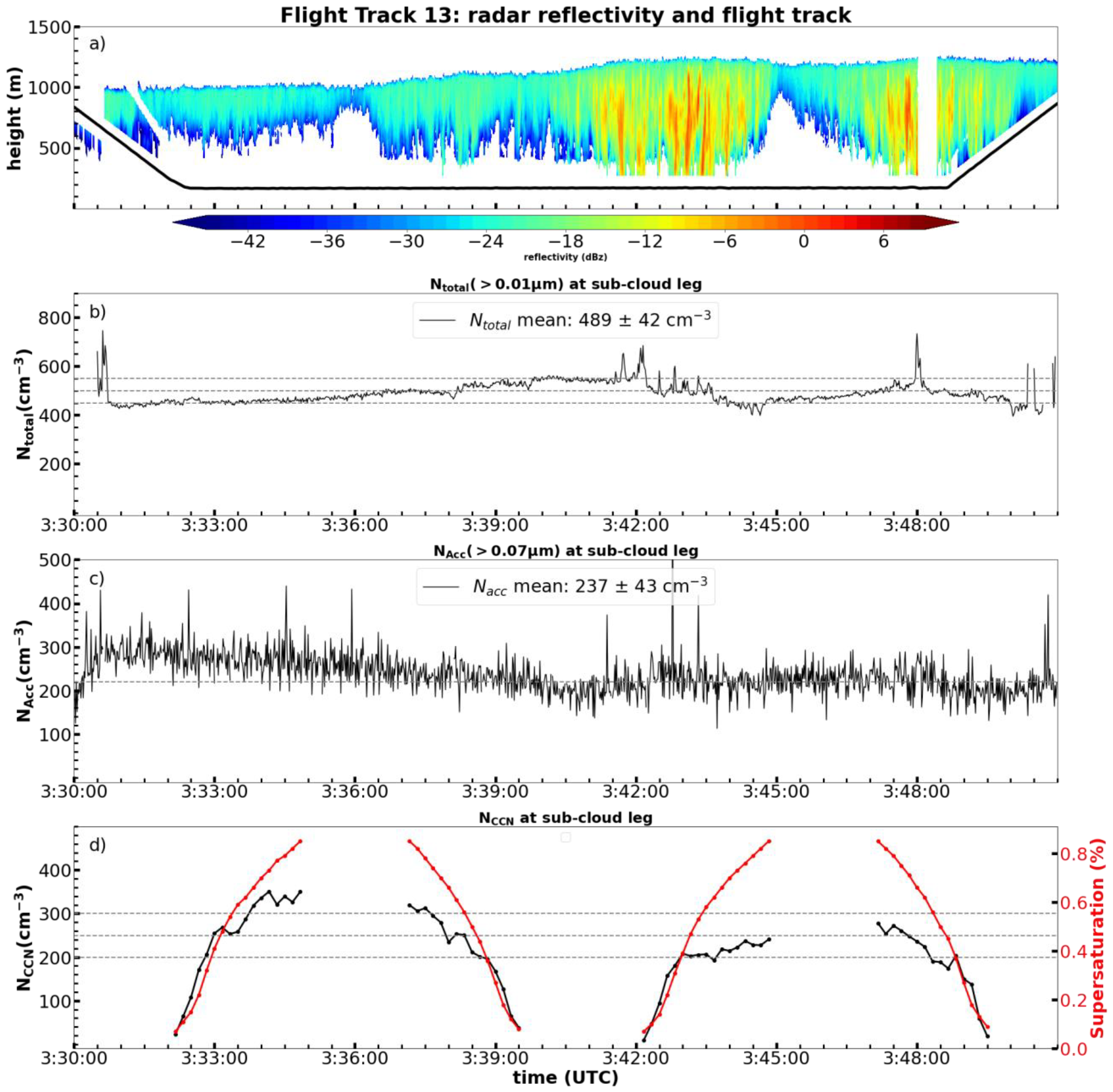
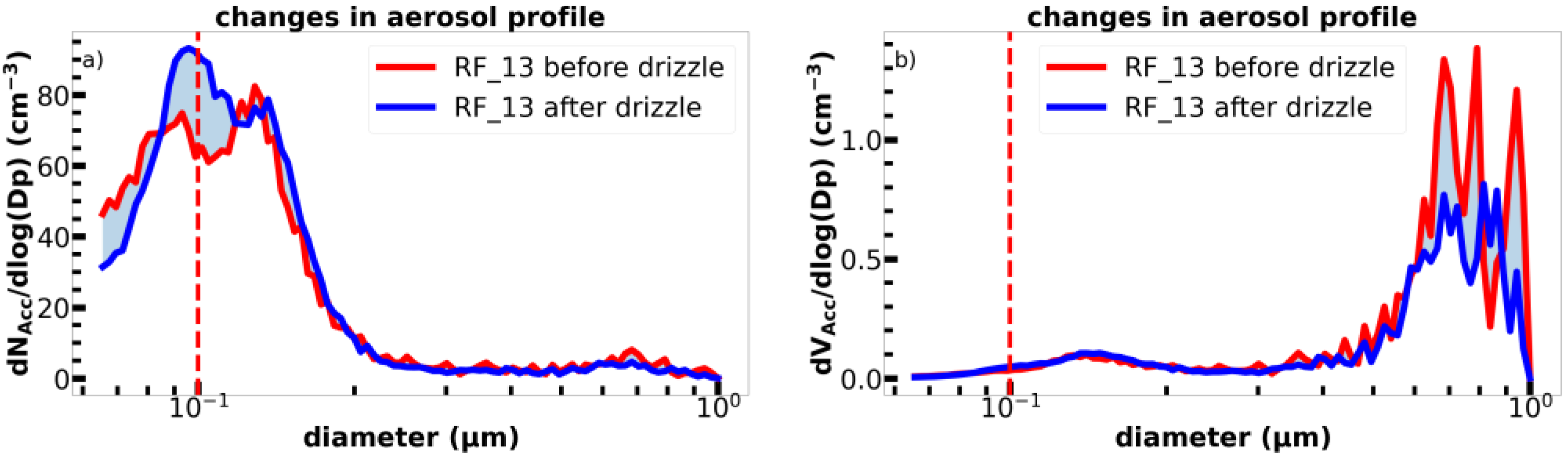
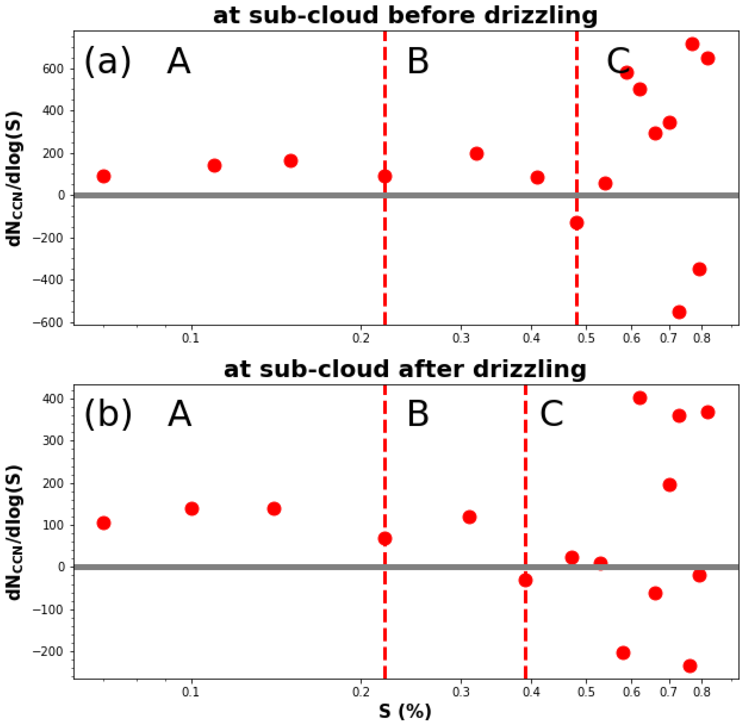
• A research flight case (Research Flight 13) was selected to demonstrate the HCR radar and in situ measurements obtained onboard research aircraft during SOCRATES including two sub-cloud periods: ‘before drizzle’ and ‘after drizzle’. Sub-cloud drizzle impacts are more evident in the presence of Aitken-mode aerosols than accumulation-mode aerosols. There was a nearly linear increase in N_CCN with supersaturation (S) during the ‘before drizzle’ period, but this was not true during the ‘after drizzle’ period, particularly when S > 0.4%, due to the precipitation scavenging effect. The effective S of the sub-cloud aerosols is nearly 0.32%, which is higher than the Hoppel minimum (0.22% S). This suggests that all the accumulation-mode aerosols (80% of the total activated aerosols) and 20% of the sea-spray aerosols presented in the sub-cloud regime can be converted into CCN and, subsequently, cloud droplets.
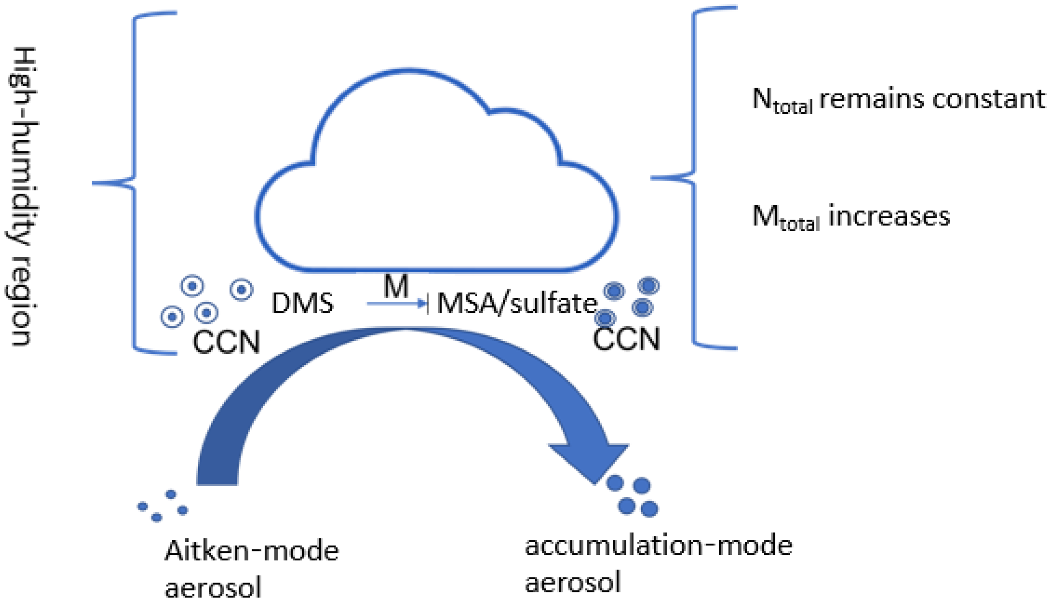
• Physical and chemical cloud processing plays an important role in aerosol size enhancement and cloud formation, especially over the SO. The aqueous-phase oxidation of DMS in the chemical cloud-processing mechanism can lead to the enlargement of the aerosol size but stasis of the aerosol number concentration. The oxidization of sulfate aerosols plays a key role in this process, and this oxidation mechanism generates sulfur species. Using the hygroscopicity parameter (κ) to quantitatively investigate the chemical cloud-processing mechanisms, we found that higher κ values (>0.4) represent cloud-processing aerosols, while lower κ values (0.1–0.2) represent the mixing of sulfate and sea-spray aerosols. The lowest value (<0.1) represents the non-cloud-processed aerosol. When the supersaturation is less than the Hoppel minimum, cloud processing is dominant, whereas sea-spray aerosols are dominant when S is 0.22%–0.32%. While these are non-cloud-processing aerosols, they are large enough to form cloud droplets, and their κ values are normally less than cloud-processed aerosols (κ~0.4) but greater than newly formed aerosols (κ ~ 0.09).
• A schematic diagram (Figure 5) was drawn to illustrate the cloud-processing mechanism where the newly formed aerosols in the FT descend into the sub-cloud layer due to high turbulence and the small particles are convected into the cloud layer and then evaporated to become accumulation-mode aerosols following the experience of physical and chemical cloud processing. Physical processing, such as Brownian scavenging by the clouds, can reduce the N_Ait (N_total − N_Acc) (shown in Figure 1b,c before and after 3:42 UTC), while chemical processing enlarges the aerosol size (shown in Figure 6). The sea-spray aerosol from the sea surface also provides 20% of the accumulation that can form CCN.
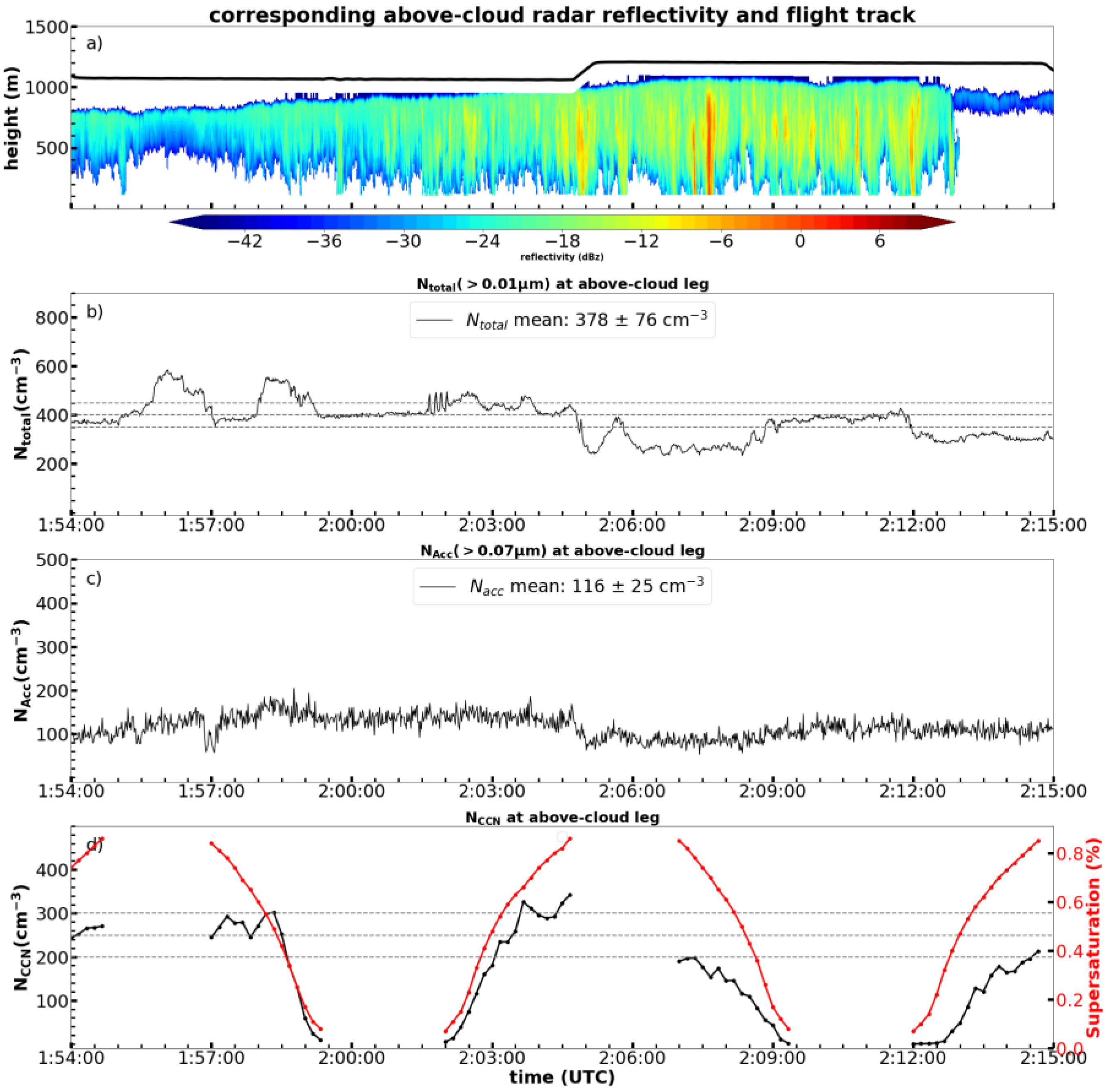
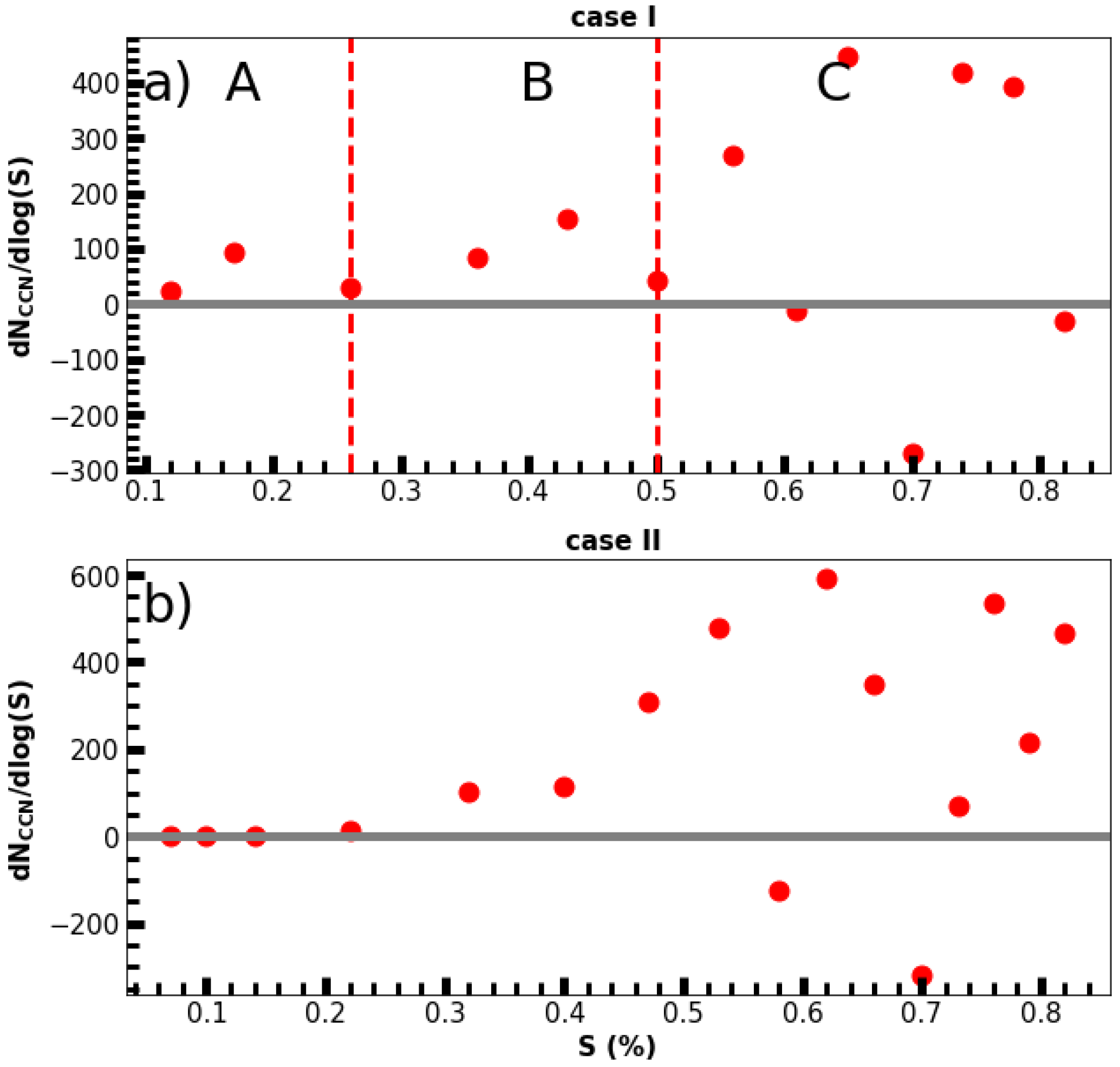
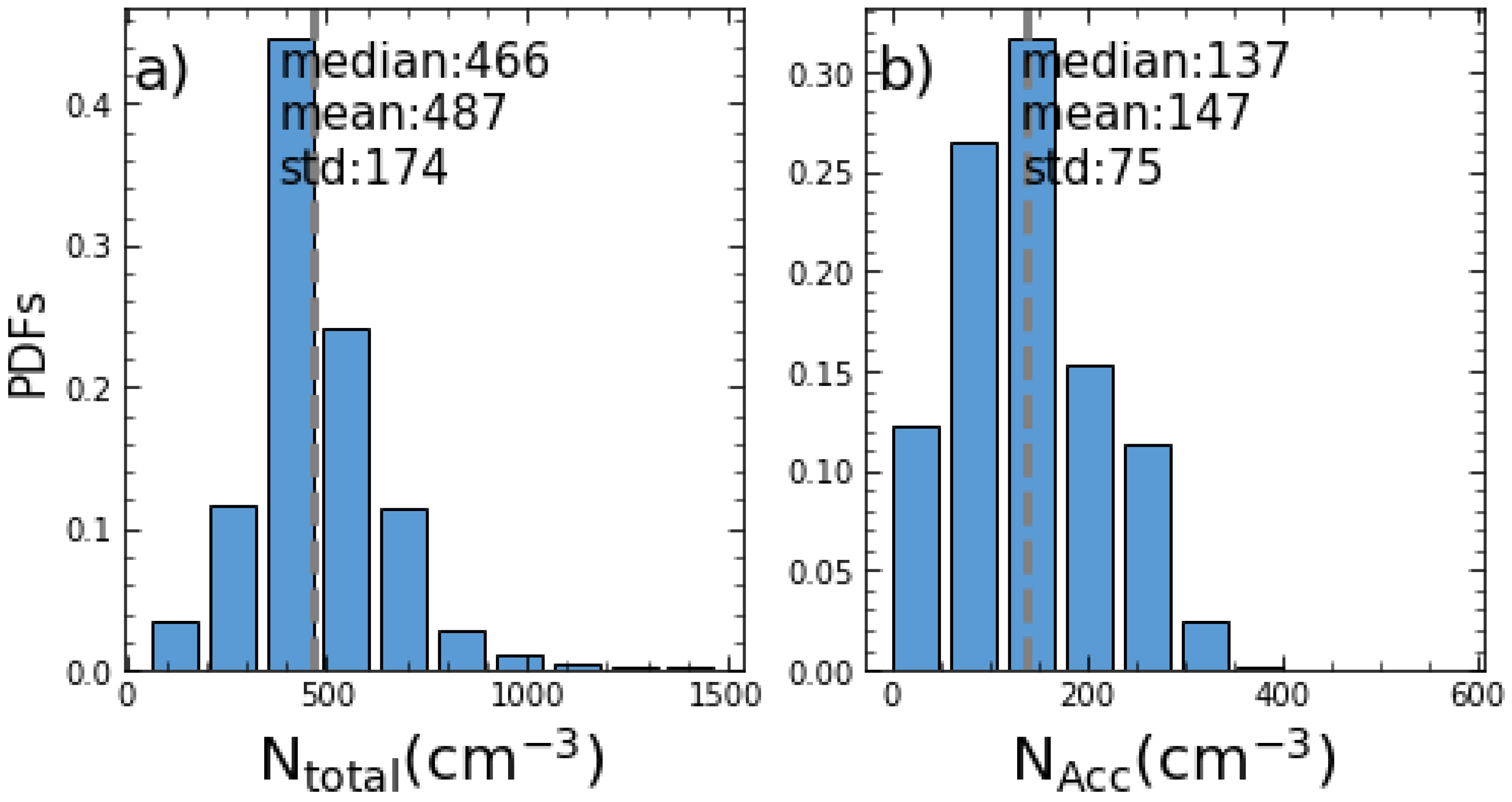
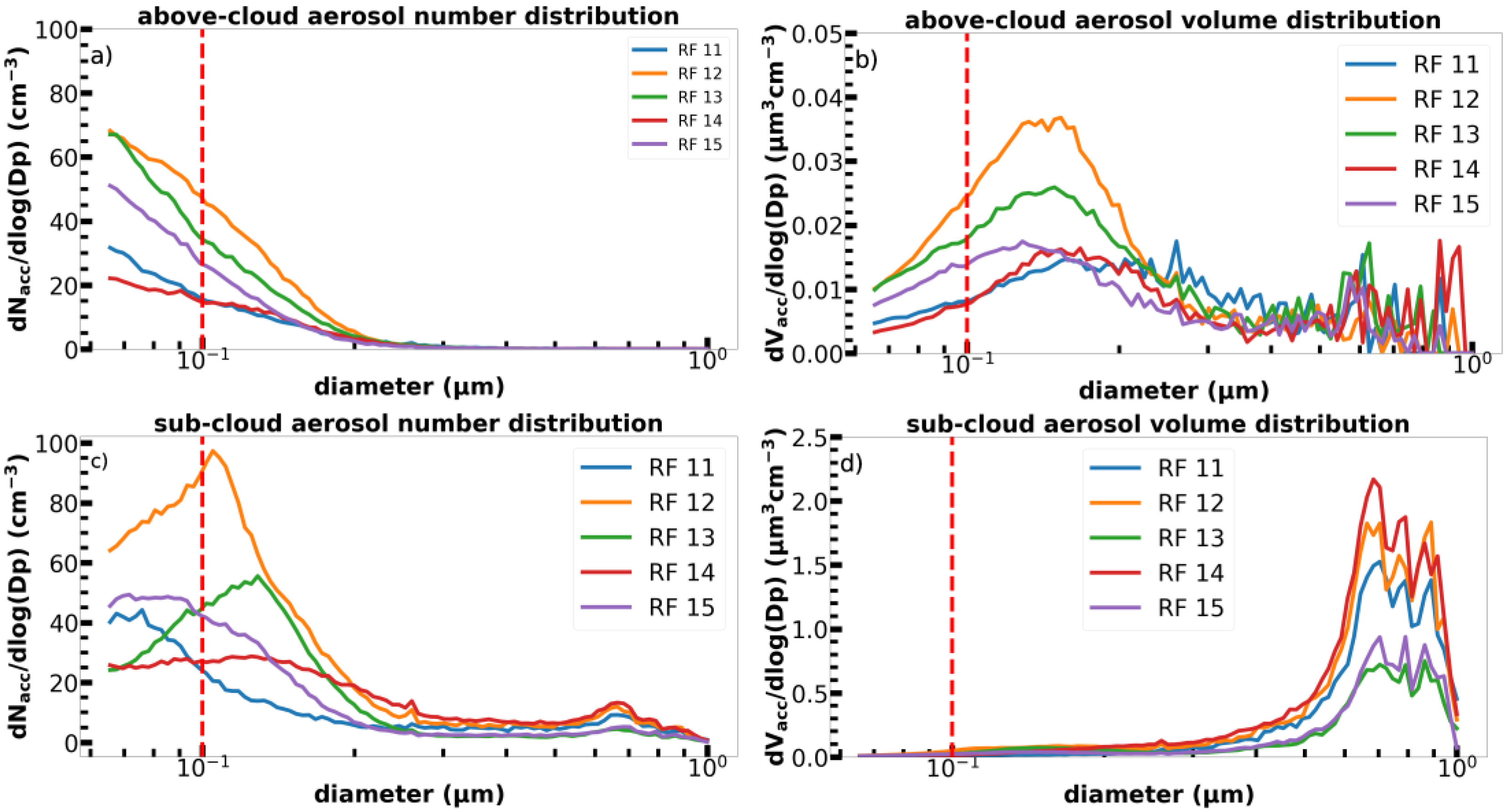
• Five cases were selected that were conducted at or below an altitude of 200 m without precipitation influence during the SOCRATES field campaign. The median and mean of N_total are 466 and 487 cm⁻³, respectively, while those of the N_Acc are 137 and 147 cm⁻³, respectively. The accumulation-mode aerosols contributed approximately 30% of the total aerosols from the five selected cases, indicating that the Aitken-mode aerosols contributed approximately 70% of the total aerosols in this study. The peaks of aerosol number and volume size distribution in the above-cloud regime are at <0.07 μm and 0.12 μm in diameter, respectively. In contrast, those in the sub-cloud regime are at 0.1 μm and 0.9 μm.

This study primarily investigates the aerosol and CCN properties for above- and sub-cloud regimes, ‘before drizzle’ and ‘after drizzle’ periods, and cloud-processing mechanisms over the Southern Ocean using the in situ measurements from five selected cases. These results provide valuable information for the community on MBL aerosols, CCN, and the cloud-processing mechanisms over the SO and have the potential to enhance our understanding and analysis of aerosol and CCN properties, while also offering insights for improving model simulations specifically focused on the Southern Ocean. However, it is important to note that further studies with more cases are necessary to draw more robust conclusions in the future.

References

1. Suzuki, K.; Nakajima, T.Y.; Stephens, G.L. Particle Growth and Drop Collection Efficiency of Warm Clouds as Inferred from Joint CloudSat and MODIS Observations. J. Atmos. Sci. 2010, 67, 3019–3032. [Google Scholar] [CrossRef]
2. Wood, R.; Kubar, T.; Hartmann, D. Understanding the importance of microphysics and macrophysics for warm rain in marine low clouds. Part II: Heuristic models of rain formation. J. Atmos. Sci. 2009, 66, 2973–2990. [Google Scholar] [CrossRef]
3. Nakajima, T.Y.; Suzuki, K.; Stephens, G.L. Droplet growth in warm water clouds observed by the A-Train. Part I: Sensitivity analysis of the MODIS-derived cloud droplet sizes. J. Atmos. Sci. 2010, 67, 1884–1896. [Google Scholar] [CrossRef]
4. Nakajima, T.Y.; Suzuki, K.; Stephens, G.L. Droplet growth in warm water clouds observed by the A-Train. Part II: A multi-sensor view. J. Atmos. Sci. 2010, 67, 1897–1907. [Google Scholar] [CrossRef]
5. Wood, R.; Hartmann, D.L. Spatial variability of liquid water path in marine low cloud: The importance of mesoscale cellular convection. J. Clim. 2006, 19, 1748–1764. [Google Scholar] [CrossRef]
6. Cherian, R.; Quaas, J. Trends in AOD, Clouds, and Cloud Radiative Effects in Satellite Data and CMIP5 and CMIP6 Model Simulations Over Aerosol Source Regions. Geophys. Res. Lett. 2020, 47, e2020GL087132. [Google Scholar] [CrossRef]
7. Jiang, J.H.; Su, H.; Wu, L.; Zhai, C.; Schiro, K.A. Improvements in Cloud and Water Vapor Simulations Over the Tropical Oceans in CMIP6 Compared to CMIP5. Earth Space Sci. 2021, 8, e2020EA001520. [Google Scholar] [CrossRef]
8. Zheng, X.; Tao, C.; Zhang, C.; Xie, S.; Zhang, Y.; Xi, B.; Dong, X. Assessment of CMIP5 and CMIP6 AMIP simulated clouds and surface shortwave radiation using ARM observations over different climate regions. J. Clim. 2023. in review. [Google Scholar]
9. Flato, G.; Marotzke, J.; Abiodun, B.; Braconnot, P.; Chou, S.C.; Collins, W.; Cox, P.; Driouech, F.; Emori, S.; Eyring, V.; et al. Evaluation of Climate Models. In Climate Change 2013: The Physical Science Basis. Contribution of Working Group I to the Fifth Assessment Report of the Intergovernmental Panel on Climate Change; Stocker, T.F., Qin, D., Plattner, G.-K., Tignor, M., Allen, S.K., Boschung, J., Nauels, A., Xia, Y., Bex, V., Midgley, P.M., Eds.; Cambridge University Press: Cambridge, UK; New York, NY, USA, 2013. [Google Scholar]
10. IPCC. Climate Change 2021: The Physical Science Basis; Masson-Delmotte, V., Zhai, P., Pirani, A., Connors, S.L., Péan, C., Chen, Y., Goldfarb, L., Gomis, M.I., Matthews, J.B.R., Berger, S., et al., Eds.; Cambridge University Press: Cambridge, UK, 2021; p. 2391. [Google Scholar]
11. Zhao, L.; Wang, Y.; Zhao, C.; Dong, X.; Yung, Y.L. Compensating Errors in Cloud Radiative and Physical Properties over the Southern Ocean in the CMIP6 Climate Models. Adv. Atmos. Sci. 2022, 39, 2156–2171. [Google Scholar] [CrossRef]
12. Mace, G.G.; Zhang, Q.; Vaughan, M.; Marchand, R.; Stephens, G.; Trepte, C.; Winker, D. A description of hydrometeor layer occurrence statistics derived from the first year of merged Cloudsat and CALIPSO data. J. Geophys. Res. 2009, 114, D00A26. [Google Scholar] [CrossRef]
13. Chubb, T.; Jensen, J.B.; Siems, S.T.; Manton, M.J. In situ observations of supercooled liquid clouds over the Southern Ocean during the HIAPER Pole-to-Pole Observation campaigns. Geophys. Res. Lett. 2013, 40, 5280–5285. [Google Scholar] [CrossRef]
14. Carslaw, K.S.; Lee, L.A.; Reddington, C.L.; Pringle, K.J.; Rap, A.; Forster, P.M.; Mann, G.W.; Spracklen, D.V.; Woodhouse, M.T.; Regayre, L.A.; et al. Large contribution of natural aerosols to uncertainty in indirect forcing. Nature 2013, 503, 67–71. [Google Scholar] [CrossRef]
15. McCoy, D.T.; Burrows, S.M.; Wood, R.; Grosvenor, D.P.; Elliott, S.M.; Ma, P.-L.; Rasch, P.J.; Hartmann, D.L. Natural aerosols explain seasonal and spatial patterns of Southern Ocean cloud albedo. Sci. Adv. 2015, 1, e1500157. [Google Scholar] [CrossRef] [PubMed]
16. Saliba, G.; Chen, C.L.; Lewis, S.; Russell, L.M.; Rivellini, L.H.; Lee, A.K.Y.; Quinn, P.K.; Bates, T.S.; Haëntjens, N.; Boss, E.S.; et al. Factors driving the seasonal and hourly variability of sea-spray aerosol number in the North Atlantic. Proc. Natl. Acad. Sci. USA 2019, 116, 20309–20314. [Google Scholar] [CrossRef] [PubMed]
17. Bates, T.S.; Kapustin, V.N.; Quinn, P.K.; Covert, D.S.; Coffman, D.J.; Mari, C.; Durkee, P.A.; De Bruyn, W.J.; Saltzman, E.S. Processes controlling the distribution of aerosol particles in the lower marine boundary layer during the First Aerosol Characterization Experiment (ACE 1). J. Geophys. Res. 1998, 103, 16369–16383. [Google Scholar] [CrossRef]
18. O’Dowd, C.; Smith, M.; Consterdine, I.; Lowe, J. Marine aerosol, sea-salt, and the marine sulphur cycle: A short review. Atmos. Environ. 1997, 31, 73–80. [Google Scholar] [CrossRef]
19. Almeida, J.; Schobesberger, S.; Kuerten, A.; Ortega, I.K.; Kupiainen-Määttä, O.; Praplan, A.P.; Adamov, A.; Amorim, A.; Bianchi, F.; Breitenlechner, M.; et al. Molecular understanding of sulphuric acid-amine particle nucleation in the atmosphere. Nature 2013, 502, 359. [Google Scholar] [CrossRef]
20. Woodhouse, M.T.; Carslaw, K.S.; Mann, G.W.; Vallina, S.M.; Vogt, M.; Halloran, P.R.; Boucher, O. Low sensitivity of cloud condensation nuclei to changes in the sea-air flux of dimethyl-sulphide. Atmos. Chem. Phys. 2010, 10, 7545–7559. [Google Scholar] [CrossRef]
21. Ayers, G.P.; Gillett, R.W. DMS and its oxidation products in the remote marine atmosphere: Implications for climate and atmospheric chemistry. J. Sea Res. 2000, 43, 275–286. [Google Scholar] [CrossRef]
22. Ayers, G.P.; Gras, J.L. Seasonal relationship between cloud condensation nuclei and aerosol methanesulphonate in marine air. Nature 1991, 353, 834–835. [Google Scholar] [CrossRef]
23. Sanchez, K.J.; Roberts, G.C.; Saliba, G.; Russell, L.M.; Twohy, C.; Reeves, M.J.; Humphries, R.S.; Keywood, M.D.; Ward, J.P.; McRobert, I.M. Measurement report: Cloud processes and the transport of biological emissions affect Southern Ocean particle and cloud condensation nuclei concentrations. Atmos. Chem. Phys. 2021, 21, 3427–3446. [Google Scholar] [CrossRef]
24. McCoy, I.L.; Bretherton, C.S.; Wood, R.; Twohy, C.H.; Gettelman, A.; Bardeen, C.G.; Toohey, D.W. Influences of recent particle formation on southern ocean aerosol variability and low cloud properties. J. Geophys. Res. Atmos. 2021, 126, e2020JD033529. [Google Scholar] [CrossRef]
25. Thornton, D.C.; Bandy, A.R.; Blomquist, B.W.; Bradshaw, J.D.; Blake, D.R. Vertical transport of sulfur dioxide and dimethyl sulfide in deep convection and its role in new particle formation. J. Geophys. Res. 1997, 102, 28501–28509. [Google Scholar] [CrossRef]
26. McFarquhar, G.M.; Bretherton, C.S.; Marchand, R.; Protat, A.; DeMott, P.J.; Alexander, S.P.; Roberts, G.C.; Twohy, C.H.; Toohey, D.; Siems, S.; et al. Observations of Clouds, Aerosols, Precipitation, and Surface Radiation over the Southern Ocean: An Overview of CAPRICORN, MARCUS, MICRE, and SOCRATES. Bull. Am. Meteorol. Soc. 2021, 102, E894–E928. [Google Scholar] [CrossRef]
27. Chen, Q.; Sherwen, T.; Evans, M.; Alexander, B. DMS oxidation and sulfur aerosol formation in the marine troposphere: A focus on reactive halogen and multiphase chemistry. Atmos. Chem. Phys. 2018, 18, 13617–13637. [Google Scholar] [CrossRef]
28. Hoppel, W.A.; Frick, G.M.; Fitzgerald, J.W.; Larson, R.E. Marine boundary layer measurements of new particle formation and the effects nonprecipitating clouds have on aerosol size distribution. J. Geophys. Res. 1994, 99, 14443–14459. [Google Scholar] [CrossRef]
29. Sharon, T.M.; Albrecht, B.A.; Jonsson, H.H.; Minnis, P.; Khaiyer, M.M.; van Reken, T.M.; Seinfeld, J.; Flagan, R. Aerosol and cloud microphysical characteristics of rifts and gradients in maritime stratocumulus clouds. J. Atmos. Sci. 2006, 63, 983–997. [Google Scholar] [CrossRef]
30. Hoppel, W.A.; Fitzgerald, J.W.; Frick, G.M.; Larson, R.E. Aerosol Size Distributions and Optical Properties Found in the Marine Boundary Layer Over the Atlantic Ocean. J. Geophys. Res. 1990, 95, 3659–3686. [Google Scholar] [CrossRef]
31. Hudson, J.G.; Noble, S.; Tabor, S. Cloud supersaturations from CCN spectra Hoppel minima. J. Geophys. Res. Atmos. 2015, 120, 3436–3452. [Google Scholar] [CrossRef]
32. UCAR/NCAR—Earth Observing Laboratory. SOCRATES: Low Rate (LRT—1 sps) Navigation, State Parameter, and Microphysics Flight-Level Data. Version 1.4. UCAR/NCAR—Earth Observing Laboratory. 2022. Available online: https://data.eol.ucar.edu/dataset/552.002 (accessed on 13 July 2023).
33. Sanchez, K.; Roberts, G. SOCRATES CCN measurements. Version 1.1 (Version 1.1) [Data Set]. UCAR/NCAR—Earth Observing Laboratory. 2018. Available online: https://data.eol.ucar.edu/dataset/552.013 (accessed on 13 July 2023).
34. Petters, M.D.; Kreidenweis, S.M. A single parameter representation of hygroscopic growth and cloud condensation nucleus activity. Atmos. Chem. Phys. 2007, 7, 1961–1971. [Google Scholar] [CrossRef]
35. Twohy, C.H.; DeMott, P.J.; Russell, L.M.; Toohey, D.W.; Rainwater, B.; Geiss, R.; Sanchez, K.J.; Lewis, S.; Roberts, G.C.; Humphries, R.S.; et al. Cloud nucleating particles over the Southern Ocean in a changing climate. Earth’s Future 2021, 9, e2020EF001673. [Google Scholar] [CrossRef]
36. Wang, Y.; Zhao, C.; McFarquhar, G.M.; Wu, W.; Reeves, M.; Li, J. Dispersion of droplet size distributions in supercooled non-precipitating stratocumulus from aircraft observations obtained during the Southern Ocean Cloud Radiation Aerosol Transport Experimental Study. J. Geophys. Res. Atmos. 2021, 126, e2020JD033720. [Google Scholar] [CrossRef]
37. McComiskey, A.; Feingold, G.; Frisch, A.S.; Turner, D.D.; Miller, M.A.; Chiu, J.C.; Min, Q.; Ogern, J.A. An assessment of aerosol-cloud interactions in marine stratus clouds based on surface remote sensing. J. Geophys. Res. Atmos. 2009, 114, D09203. [Google Scholar] [CrossRef]
38. Wang, Y.; McFarquhar, G.M.; Rauber, R.M.; Zhao, C.; Wu, W.; Finlon, J.A.; Toohey, D.W. Microphysical properties of generating cells over the Southern Ocean: Results from SOCRATES. J. Geophys. Res. Atmos. 2020, 125, e2019JD032237. [Google Scholar] [CrossRef]
39. Wood, R. Drizzle in Stratiform Boundary Layer Clouds. Part I: Vertical and Horizontal Structure. J. Atmos. Sci. 2005, 62, 3011–3033. [Google Scholar] [CrossRef]
40. Zheng, X.; Dong, X.; Ward, D.M.; Xi, B.; Wu, P.; Wang, Y. Aerosol-Cloud-Precipitation Interactions in a Closed-cell and Non-homogenous MBL Stratocumulus Cloud. Adv. Atmos. Sci. 2023, 39, 2107–2123. [Google Scholar] [CrossRef]
41. Zhao, C.; Zhao, L.; Dong, X. A Case Study of Stratus Cloud Properties Using In Situ Aircraft Observations over Huanghua, China. Atmosphere 2019, 10, 19. [Google Scholar] [CrossRef]
42. NCAR/EOL HCR Team; NCAR/EOL HSRL Team. SOCRATES: NCAR HCR Radar and HSRL Lidar Moments Data. Version 3.1. UCAR/NCAR—Earth Observing Laboratory. 2022. Available online: https://data.eol.ucar.edu/dataset/552.034 (accessed on 13 July 2023).
43. Wu, P.; Dong, X.; Xi, B.; Tian, J.; Ward, D.M. Profiles of MBL Cloud and Drizzle Microphysical Properties Retrieved From Ground-Based Observations and Validated by Aircraft In Situ Measurements Over the Azores. J. Geophys. Res. Atmos. 2020, 125, e2019JD032205. [Google Scholar] [CrossRef]
44. Marcovercchio, A.; Xi, B.; Zheng, X.; Wu, P.; Dong, X.; Behrangi, A. What are the similarities and differences in maritime aerosol, cloud, and drizzle microphysical properties in spring and summer for Boreal and Austral mid-latitude regions? JGR Atmos. 2023. in review. [Google Scholar]
45. Filonchyk, M.; Yan, H.; Zhang, Z.; Yang, S.; Li, W.; Li, Y. Combined use of satellite and surface observations to study aerosol optical depth in different regions of China. Sci. Rep. 2019, 9, 6174. [Google Scholar] [CrossRef]
46. Zhang, J.; Zhou, Q.; Shen, X.; Li, Y. Cloud Detection in High-Resolution Remote Sensing Images Using Multi-features of Ground Objects. J. Geovis. Spat. Anal. 2019, 3, 14. [Google Scholar] [CrossRef]
47. Albrecht, B.; Fang, M.; Ghate, V. Exploring stratocumulus cloud-top entrainment processes and parameterizations by using Doppler cloud radar observations. J. Atmos. Sci. 2016, 73, 729–742. [Google Scholar] [CrossRef]
48. Bretherton, C.S.; Blossey, P.N. Low cloud reduction in a greenhouse-warmed climate: Results from Lagrangian LES of a subtropical marine cloudiness transition. J. Adv. Model. Earth Syst. 2014, 6, 91–114. [Google Scholar] [CrossRef]
49. Modini, R.L.; Frossard, A.A.; Ahlm, L.; Russell, L.M.; Corrigan, C.E.; Roberts, G.C.; Hawkins, L.N.; Schroder, J.C.; Bertram, A.K.; Zhao, R.; et al. Primary marine aerosol-cloud interactions off the coast of California. J. Geophys. Res. Atmos. 2015, 120, 4282–4303. [Google Scholar] [CrossRef]
50. Woodhouse, M.T.; Mann, G.W.; Carslaw, K.S.; Boucher, O. Sensitivity of cloud condensation nuclei to regional changes in dimethyl-sulphide emissions. Atmos. Chem. Phys. 2013, 13, 2723–2733. [Google Scholar] [CrossRef]
51. Saliba, G.; Sanchez, K.J.; Russell, L.M.; Twohy, C.H.; Roberts, G.C.; Lewis, S.; Dedrick, J.; McCluskey, C.S.; Moore, K.; DeMott, P.J.; et al. Organic composition of three different size ranges of aerosol particles over the Southern Ocean. Aerosol Sci. Technol. 2020, 55, 268–288. [Google Scholar] [CrossRef]
52. Bikkina, P.; Kawamura, K.; Bikkina, S.; Kunwar, B.; Tanaka, K.; Suzuki, K. Hydroxy fatty acids in remote marine aerosols over the Pacific Ocean: Impact of biological activity and wind speed. ACS Earth Space Chem. 2019, 3, 366–379. [Google Scholar] [CrossRef]
53. Sullivan, R.C.; Petters, M.D.; Demott, P.J.; Kreidenweis, S.M.; Wex, H.; Niedermeier, D.; Hartmann, S.; Clauss, T.; Stratmann, F.; Reitz, P.; et al. Irreversible loss of ice nucleation active sites in mineral dust particles caused by sulphuric acid condensation. Atmos. Chem. Phys. 2010, 10, 11471–11487. [Google Scholar] [CrossRef]
54. Zieger, P.; Väisänen, O.; Corbin, J.C.; Partridge, D.G.; Bastelberger, S.; Mousavi-Fard, M.; Rosati, B.; Gysel, M.; Krieger, U.K.; Leck, C.; et al. Revising the hygroscopicity of inorganic sea salt particles. Nat. Commun. 2017, 8, 15883. [Google Scholar] [CrossRef]
Figure 1. (a) Cloud radar reflectivity (contour) onboard aircraft and RF13 aircraft flight track (black line) between 3:30 to 3:52 UTC during SOCRATES. Time series of (b) total particle number concentration Ntotal, (c) accumulation-mode aerosol number concentration NAcc, and (d) cloud condensation nuclei concentration NCCN collected at the sub-cloud aircraft horizontal leg.
Atmosphere 14 01246 g001
Figure 2. Himawari-8-satellite-retrieved cloud optical depths (CODs) during different time periods of RF13: (a) 03:20, (b) 03:30, (c) 03:40, and (d) 03:50 UTC. The horizontal flight tracks are overlayed as a solid line and represent the same portion of flight track shown in this figure (red lines represent the first half and blue lines represent the second half). All panels display an area from 51° S to 53° S and 156° E to 158° E, which covers the selected portion of flight path.
Atmosphere 14 01246 g002
Figure 3. (a) Above-cloud aerosol and CCN properties during RF13. Time series of (b) total particle number concentration Ntotal, (c) accumulation-mode aerosol number concentration NAcc, and (d) cloud condensation nuclei concentration NCCN.
Atmosphere 14 01246 g003
Figure 4. DMS mixing ratios from MERRA2 at 03:00 UTC, 18 February 2018. The white color represents the location with DMS mixing ratios < 100 ppt. The larger red rectangle represents the location of the whole SOCRATES field campaign, while the smaller rectangle in the sub-plot represents the location of flight tracks.
Atmosphere 14 01246 g004
Figure 5. A schematic diagram to illustrate the chemical cloud-processing mechanism for large Aitken-mode aerosols to form accumulation-mode aerosols.
Atmosphere 14 01246 g005
Figure 6. The RF13 accumulation-mode aerosol (a) number and (b) volume distributions during the ‘before drizzle’ and ‘after drizzle’ periods. A vertical dash line at 0.1 μm diameter is present.
Atmosphere 14 01246 g006
Figure 7. Differential CCN concentrations ((NCCN(S + ∆S) − NCCN(S))/(log(S + ∆S) − log(S))) against critical supersaturation (S) over (a) sub-cloud ‘before drizzle’ period and (b) sub-cloud ‘after drizzle’ period, same as in Figure 1. The entire supersaturation range is classified into 3 three regimes denoted as A, B, and C based on the local minimum of differential CCN spectra values (dN/dlog(S) at S = S1 is lower than those at adjacent values S = S1 + ∆S and S = S1 − ∆S). Gray solid line marks 0. Vertical red dash lines show the local minimum of CCN spectra values.
Atmosphere 14 01246 g007
Figure 8. Cloud droplet number concentration from the cloud above the flight track during the (a) ‘before drizzle’ and (b) ‘after drizzle’ periods.
Atmosphere 14 01246 g008
Figure 9. Two differential CCN concentrations against critical supersaturation in above-cloud regime. The case (a) was selected from 2:07–2:10 UTC, the case (b) was selected from 2:11–2:15 UTC. Gray solid line marks 0. Vertical red dash lines show the local minimum of CCN spectra values.
Atmosphere 14 01246 g009
Figure 10. (a) Probability density functions (PDFs) and statistical results of the CPC-measured total aerosol number concentration (Ntotal, D > 0.01 µm) and (b) UHSAS-measured accumulation-mode aerosols (NAcc, D > 0.07 µm) for the sub-cloud regimes of the five selected cases (RF11–15, 11,362 1 s samples) during SOCRATES. Gray dashed line marks the median of variables.
Atmosphere 14 01246 g010
Figure 11. The above-cloud accumulation-mode aerosol size distributions by (a) number and (b) volume from five selected cases; (c) and (d) are the same as (a) and (b) except for the sub-cloud aerosol size number and volume distributions. Red dashed line marks 0.1 μm.
Atmosphere 14 01246 g011
Disclaimer/Publisher’s Note: The statements, opinions and data contained in all publications are solely those of the individual author(s) and contributor(s) and not of MDPI and/or the editor(s). MDPI and/or the editor(s) disclaim responsibility for any injury to people or property resulting from any ideas, methods, instructions or products referred to in the content.