Article

Centennial Variation and Mechanism of the Extreme High Temperatures in Summer over China during the Holocene Forced by Total Solar Irradiance

1
Key Laboratory for Virtual Geographic Environment, Ministry of Education, State Key Laboratory Cultivation Base of Geographical Environment Evolution of Jiangsu Province, Jiangsu Center for Collaborative Innovation in Geographical Information Resource Development and Application, School of Geography Science, Nanjing Normal University, Nanjing 210024, China
2
Jiangsu Provincial Key Laboratory for Numerical Simulation of Large Scale Complex Systems, School of Mathematical Science, Nanjing Normal University, Nanjing 210024, China
3
Open Studio for the Simulation of Ocean-Climate-Isotope, Qingdao National Laboratory for Marine Science and Technology, Qingdao 266100, China
4
Frontier Science Center for Deep Ocean Multispheres and Earth System (DOMES), Institute for Advanced Ocean Study (IAOS) and Physical Oceanography Laboratory (POL), Ocean University of China, Qingdao 266100, China
*
Authors to whom correspondence should be addressed.
Atmosphere 2023, 14(8), 1207; https://doi.org/10.3390/atmos14081207
Submission received: 25 June 2023 / Revised: 25 July 2023 / Accepted: 25 July 2023 / Published: 27 July 2023
(This article belongs to the Special Issue Climate Extremes in China)

Abstract

:
Under the background of global warming, the frequency and intensity of extreme climate have increased, especially extreme high temperatures. In order to correctly predict the changes in the extreme high temperatures in summer in China in this century, it is urgent to deepen the understanding of the characteristics and physical mechanisms of the extreme high temperatures in summer on the centennial timescale. Many researchers have explored the mechanism of the influences of the variability of the solar cycle on climate change, while the mechanism of the influences of the centennial variation of solar activity on climate change remains elusive. Here, we use the outputs from the Control (CTRL) experiment, Total solar irradiance and Orbital (TSI_ORB) experiment, and Orbital (ORB) experiment from Nanjing Normal University-Holocene (NNU-Hol) experiments to study the extreme high temperatures in summer in China during the Holocene. On the basis of verifying the consistency of the centennial period between the TSI (TSI_ORB minus ORB plus CTRL) experiment and the reconstructed data, we compared the centennial variation characteristics of the summer extreme high temperature in the CTRL experiment and the TSI experiment. It shows that under the modulation of total solar irradiance, the centennial spatial pattern of the summer extreme high temperatures changed from dipole mode to uniform mode, with 300-year and 500-year periodicity, compared to the influence of only internal variability. On the centennial time scale, the greatest difference is located in northeast China. The subsidence movement and the reduction of cloud cover caused by the anticyclone under the control of high-pressure lead to the increase of downward solar radiation, thus making a positive center is showed in northeast China on the impacts of total solar irradiance. Furthermore, the center of the Rossby wave train in the barotropic structure of the upper circulation related to the summer extreme high temperature significantly moves northward. This barotropic structure is composed of continuous pressure ridges from Eurasia to North America and the North Atlantic, which is conducive to the increase of the summer extreme high temperatures. Furthermore, we investigated the underlying physical mechanisms. Under the influence of total solar irradiance, the Pacific Decadal Oscillation (PDO) with the same centennial cycle as extreme high temperatures lead to obvious subsidence movement and increase of radiation flux, causing an increase in extreme high temperatures over northeast China.

1. Introduction

In recent years, with the increasing impact of extreme weather and extreme climate on the economy, environment, and society, more and more attention has been paid to its research [1,2]. Different from previous assessment reports, the sixth assessment report (AR6) of the Intergovernmental Panel on Climate Change (IPCC) is the first time to conduct a comprehensive and systematic assessment of changes in extreme climate in a separate chapter (i.e., Chapter 11) [3]. The warming of the modern climate is a major global issue of general concern in the international community, which has a far-reaching impact on the global natural ecosystem and human socio-economic development [4]. The IPCC-AR5 further confirmed the fact of global warming in the past century [5]. Compared with AR5, in AR6, with the increase of observation data, the development of climate models, and the deepening of scientific research, the evidence of extreme climate changes has been further strengthened, especially the attribution of human activities on single events, drought, tropical cyclones, and complex events has made new progress, and the reliability of the assessment conclusions has been improved [6]. However, if only human activities are considered, the impact of natural forcing factors on extreme high temperatures is ignored, and the contribution of natural factors and human factors to the change of extreme high temperatures in a century cannot be clarified.
The Holocene is the latest geological age, and its climate change is closely related to the development of human society. The existing global and regional reconstruction sequences have proven that there was a great warm period in the Holocene [7,8,9], and its climate and environmental characteristics and changes may provide a historical reference for modern global warming. Taking the great warm period in the mid-Holocene as a historical similarity for future climate change is of great scientific significance for predicting climate change under future warming scenarios. It is of great practical significance to distinguish the natural and anthropogenic impacts and promote the sustainable development of the social economy [10].
Wang et al. (2000) reconstructed the Holocene temperature series covering the whole Holocene over China [11]. They summarized and analyzed four typical periods of climate change in recent 10,000 years: Great Warm Period, Middle Ages Warm Period, Little Ice Age, and Modern Warm Period. The study found that the Great Warm Period occurred at 8.5–3.0 ka, and the warmest period occurred during the 500-year period of 5.5–6.0 ka. The temperature was more than 2 °C higher than the average in the recent 100 years. Ge et al. (2006) reconstructed the temperature change sequences of 31 sites (regions) in China based on proxy evidence such as pollen, stalagmites, lake sediments, peat, ice cores, and historical documents in the past 2000 years [12]. Using integrated methods, they reconstructed a temperature change series of China with a resolution of 100 years in the past 5000 years. The research shows that, since 5000 years ago, the entire region of China has been divided into two distinct cold and warm periods on the millennium scale, namely, the warm climate period of 3050–250 BC and the cold climate period since 250 BC. In these two millennium-scale cold and warm periods, there are obviously many secondary cold and warm fluctuation stages, such as 2850 BC, 2350 BC, 950 BC, 250 BC, and 550 BC, which are several obvious century-scale cooling stages and 2750 BC, 850 BC, and 650 AD, which are several obvious centennial-scale warming stages. At the same time, Hou et al. (2016) analyzed the characteristics of the Holocene temperature change in China [13] based on the data of the Holocene temperature integrated sequence reconstructed by Fang et al. (2011) [8] and found that the Holocene cold and warm events had significant cycles of 1000 years and 700 years, respectively.
However, the above reconstruction series are mostly average temperature series, and the research on the highest temperature is less. In order to better understand the causes and historical status of the highest temperature, and to scientifically predict the future climate change trend, the development of climate models and climate simulation research came into being. After decades of development, climate models have become an important tool for studying the mechanism of past climate change and predicting future climate change [14,15,16,17].
Ren et al. (2019) analyzed the response of global extreme temperature during the mid-Holocene Warm Period using the data from the Holocene Warm Period Experiment and the preindustrial (PI) experiment in the MPI-ESM-P air–sea coupling model [18]. The results showed that, due to the increased summer orbital solar radiation in the Northern Hemisphere compared to before the PI, the average temperature in the mid-Holocene increased in the polar oceans and the land areas in the middle and high latitudes of the Northern Hemisphere in summer, while the temperature in other regions decreased; In the regions where the average temperature increased, the extreme high and low temperatures also increased, and the frequency of warm events increased; The relative indices of daily maximum temperatures in land areas change more than those of daily minimum temperatures; Compared with the response to extreme high temperature events, the response to extreme low temperature events in polar ocean areas is more significant, the frequency of cold events is significantly reduced, and the number of days higher than 0 °C throughout the year is significantly increased. Yan et al. (2019) studied the temporal characteristics of space and 4.2 ka BP events and determine the possible causes and mechanisms behind the events by using the TraCE-21 ka data (simulating the transient climate evolution in the past 21,000 years [19]) which is a set of transient simulations using the Community Climate System Model version 3 (CCSM3). In order to determine the characteristics of 4.2 ka BP events, the 100-year cold period and two 100-year warm periods exceeding ±0.5 standard deviations were selected. The two 100-year cold periods are 4320 to 4220 BP and 4150 to 4050 BP, respectively, and the two 100-year warm periods are 4710 to 4610 BP and 3980 to 3880 BP, respectively. The Northern Hemisphere (NH) and Southern Hemisphere (SH) modes indicate that the Intertropical Convergence Zone (ITCZ) moves southward, as shown in the reconstruction. These characteristics may also be related to the weakening of the Atlantic Meridional Overturning Circulation (AMOC), which requires further investigation [20].
In terms of physical mechanism analysis, studies of the high-resolution climate records in the tropical Pacific region show that El Niño-like events have occurred and display a cyclical pattern of millennial and centennial changes [21]. This leads to the view of “low-latitude driving”, which holds that the periodic variation of low-latitude monsoon precipitation is not necessarily determined by high-latitude ice sheets. In many paleo-climate studies, the North Atlantic is considered to be one of the driving factors of monsoon change [22,23,24]. The climate change in the North Atlantic that existed throughout the Holocene is usually related to solar anomalies [25]. A detrended, composite reconstruction of North Atlantic Sea Surface Temperature (SST) that emphasizes centennial-scale variability [26] shows cooler SST during the two largest dry periods between 2800 and 2300 BC and the beginning of the prolonged dry period from 1600–400 BC at Ngamring Tso [27]. The stalagmite reconstruction results of Tan et al. (2014) show that there is a significant 127–105-year cycle of monsoon change in southern Shaanxi during 4200–1972 BC, which may be controlled by solar activity and Pacific Decadal Oscillation/Atlantic Multidecadal Oscillation (PDO/AMO) changes, respectively. Solar activity may affect climate change in southern Shaanxi by influencing the Earth’s internal climate system, such as monsoon, PDO, and AMO [28].
Previous studies on the Holocene have mainly focused on the mean state of precipitation and temperature, with few focusing on the centennial variation and the physical mechanisms of the summer extreme temperature. The possibility that solar activity may affect the Earth’s climate system had been discussed as early as in 1801 [29]. Afterwards, numerous studies have indicated statistical correlations between climate change and long-term variation of solar activity [30,31]. Much research has explored the mechanism of the influences of the variability of the solar cycle (solar maximum to solar minimum) on climate change [32,33], while the mechanism of the influences of the long-term variation of solar activity on climate change remains elusive. Solar activity is a crucial component of the natural factors, thus study of the behavior of the climate variability responding to solar irradiation may be instrumental in understanding the effects of more complex external forcing on climate systems during the Holocene.

2. Data and Methods

The simulation results based on reliable models are a good choice to study and recognize the influences of solar activity on the extreme temperature in summer over China during the Holocene on the centennial timescale. Therefore, in this study, we chose the NNU_Hol experiments (Table 1) to explore the centennial variation and physical mechanism. At the NNU_Hol experiments, the Community Earth System Model (CESM, version 1.0.3) was used to simulate the climate that accelerated 10 times during the Holocene. The CESM project is supported primarily by the National Science Foundation (NSF). Administration of the CESM is maintained by the Climate and Global Dynamics Laboratory (CGD) at the National Center for Atmospheric Research (NCAR).
The CESM1.0.3 was launched by the National Center for Atmospheric Research (NCAR) in June 2010. It is an earth system model developed on the basis of CCSM4.0. As of February 2019, the model has been updated to version 2.1.1. The CESM takes oceans, atmosphere, land surface, and the cryosphere as its main research subjects and considers atmospheric chemistry, biogeochemistry, and human development. It is widely used in the study of climate and environment evolution, the interaction between nature and humans, and the research and prediction of climate change [34,35]. The resolution of CESM1.0.3 used in this study is T31_ G37. In the atmospheric module, the horizontal resolution is 96 × 48 (Lon × Lat), with a vertical resolution of 26 layers. In the ocean module, the horizontal resolution is 116 × 100 (Lon × Lat), with a vertical resolution of 60 layers. The horizontal resolution of the ocean model is irregular, which is different from that of the atmospheric circulation model. The NNU_Hol experiments designed seven experiments, and we only used three of them, as shown in Table 1, including the CTRL experiment, the ORB experiment, and the TSI_ORB experiment. In the CTRL experiment, all forcing factors remain unchanged. The ORB experiment only changed the Earth’s orbital parameters. The TSI_ORB experiment changed the total solar irradiance [36] and also changed the Earth’s orbital parameters, making it a double forcing experiment. The TSI experiment is obtained by subtracting the ORB experiment from the TSI_ORB experiment and add CTRL experiment. In this study, we used the monthly maximum temperatures (June, July, and August) from the CTRL and TSI experiments. The highest monthly maximum temperature in June, July, and August was selected as the summer extreme high temperature.
In order to verify the reliability of the model data, the model data were compared with the reanalysis data and reconstruction data. The first analysis data are the maximum temperature data in Reanalysis 1 from the National Center for Environmental Prediction (NCEP) and the National Center for Atmospheric Research (NCAR). The NCEP1 data is the monthly data during 1950 AD to 1990 AD, with a spatial resolution of 2.5° × 2.5°. The second analysis data are the maximum temperature data in 20th Century Reanalysis (20CR) from the National Oceanic and Atmospheric Administration (NOAA) and the Cooperative Institute for Research in Environmental Sciences (CIRES). The 20CR data is the monthly data during 1851 AD to 1990 AD, with a spatial resolution of 2° × 2°. The specific information of the reconstructed data is shown in Table 2. The location information of the reconstructed data is shown in Figure 1. The reconstruction data covering the whole Holocene is marked in red, while the reconstruction data covering only a certain period of Holocene is marked in blue.

3. Results

3.1. Verification of Model Simulation Results

We compared NCEP1 with TSI data to verify the rationality of the spatial distribution of simulated data. Since the time resolution of TSI is 10 years, we processed the time resolution of the NCEP1 into 10 years, calculating the average of 10 years per month. Due to the difference in spatial resolution between TSI and NCEP1 data, we used bilinear interpolation to interpolate the resolution of TSI data to the same spatial resolution as NCEP1 data. At the same time, in order to ensure consistency of the time period, we selected the spatial distribution of the highest temperature in summer from 1950 to 1990 for comparison. The spatial distribution of the extreme high temperatures in summer over China from 1950 to 1990 (Figure 2) shows that the TSI experiment can well reproduce the spatial distribution of the mean climate state of the summer extreme high temperature in NCEP1, with a correlation coefficient of 0.31 at the 95% confidence level. The correlation coefficient here refers to the spatial correlation coefficient. When conducting t-significance testing, as the spatial data is two-dimensional (longitude and latitude), we process it into one-dimensional data (latitude-weighted average) and then subtract two from the number of longitude grid points to determine the degree of freedom. In NCEP1 and TSI, the high value appears in Xinjiang, Inner Mongolia, and Southern China, but the summer extreme high temperatures in Inner Mongolia and Xinjiang in the TSI experiment are significantly higher than that in NCEP1.
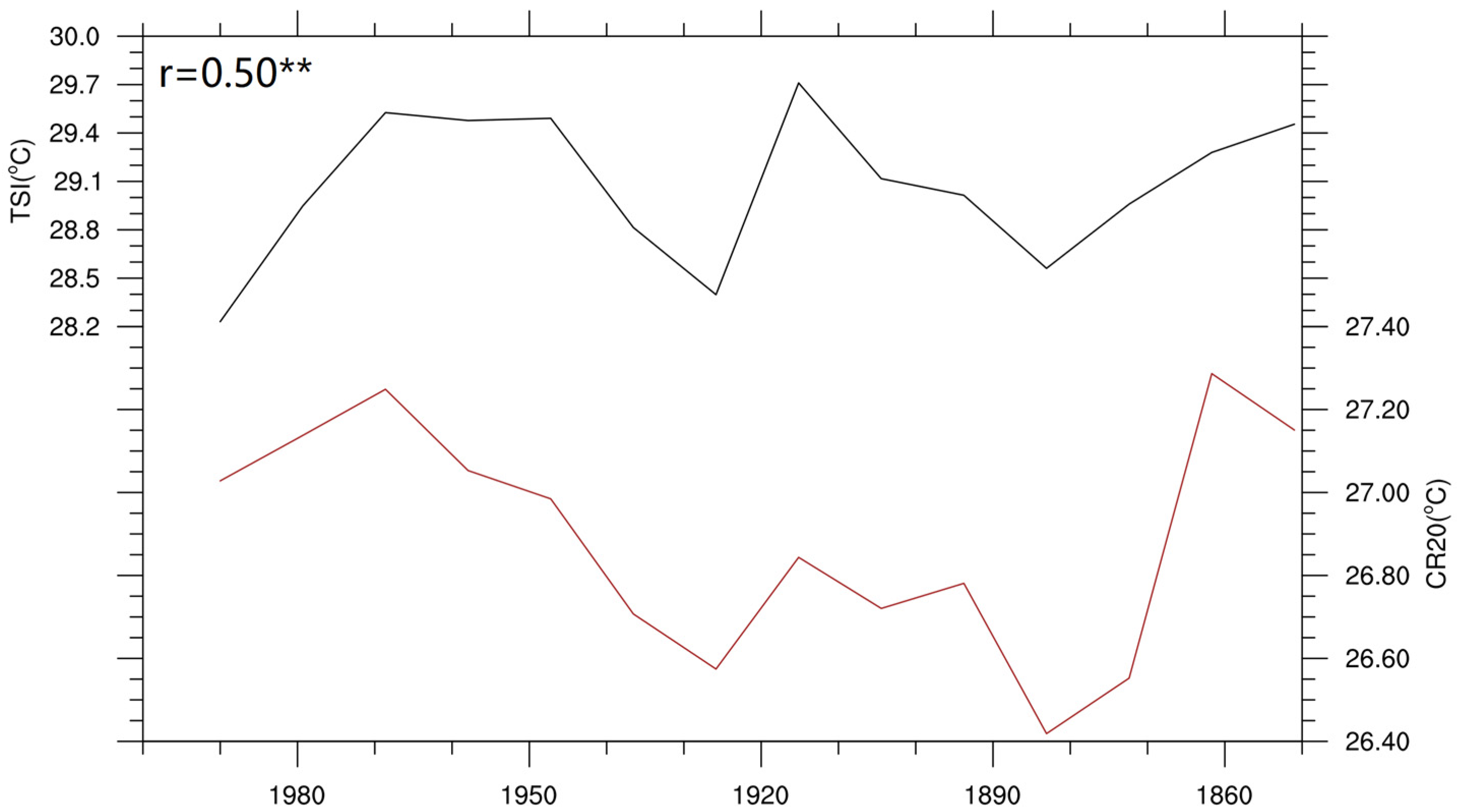
Also, we compared 20CR with TSI data using the same calculation method as NCEP1. The period being compared is from 1851 to 1990. The spatial distribution of the extreme high temperature in summer over China from 1851 to 1990 (Figure 3) shows that the spatial distribution in the TSI experiment can well reproduce the spatial distribution of the mean climate state of the summer extreme high temperature in 20CR, with a correlation coefficient of 0.35 at the 95% confidence level. In 20CR and TSI, the high value also appears in Xinjiang, Inner Mongolia and Southern China, but the summer extreme high temperature in Xinjiang in TSI experiment is also significantly higher than that in 20CR. Meanwhile, we analyzed the time series of the extreme high temperature in summer over China from 1851 to 1990 (Figure 4). Compared to the summer extreme high temperature in 20CR, although there is a numerical overestimation of the summer extreme high temperature in the TSI experiment, there is a significant correlation between the time series of summer extreme high temperature in 20CR and TSI with a correlation coefficient of 0.50 at the 95% confidence level. The correlation coefficient here refers to the temporal correlation coefficient. When conducting t-significance tests, we subtract two from the true length of the sequence to determine the degree of freedom.
In summary, the spatial distribution and time series of summer extreme high temperatures in TSI experiment are similar to them in NCEP1 and 20CR, although there are numerical overestimation in TSI experiment.
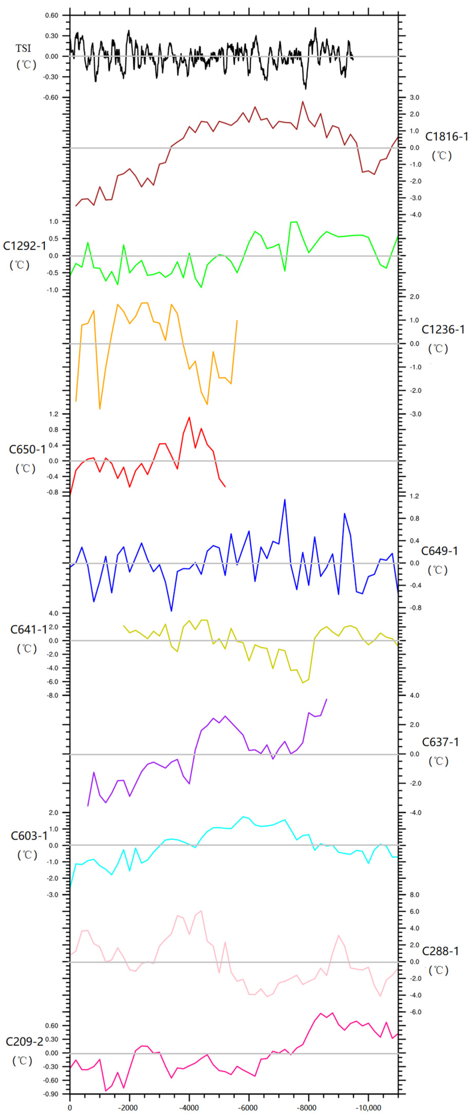
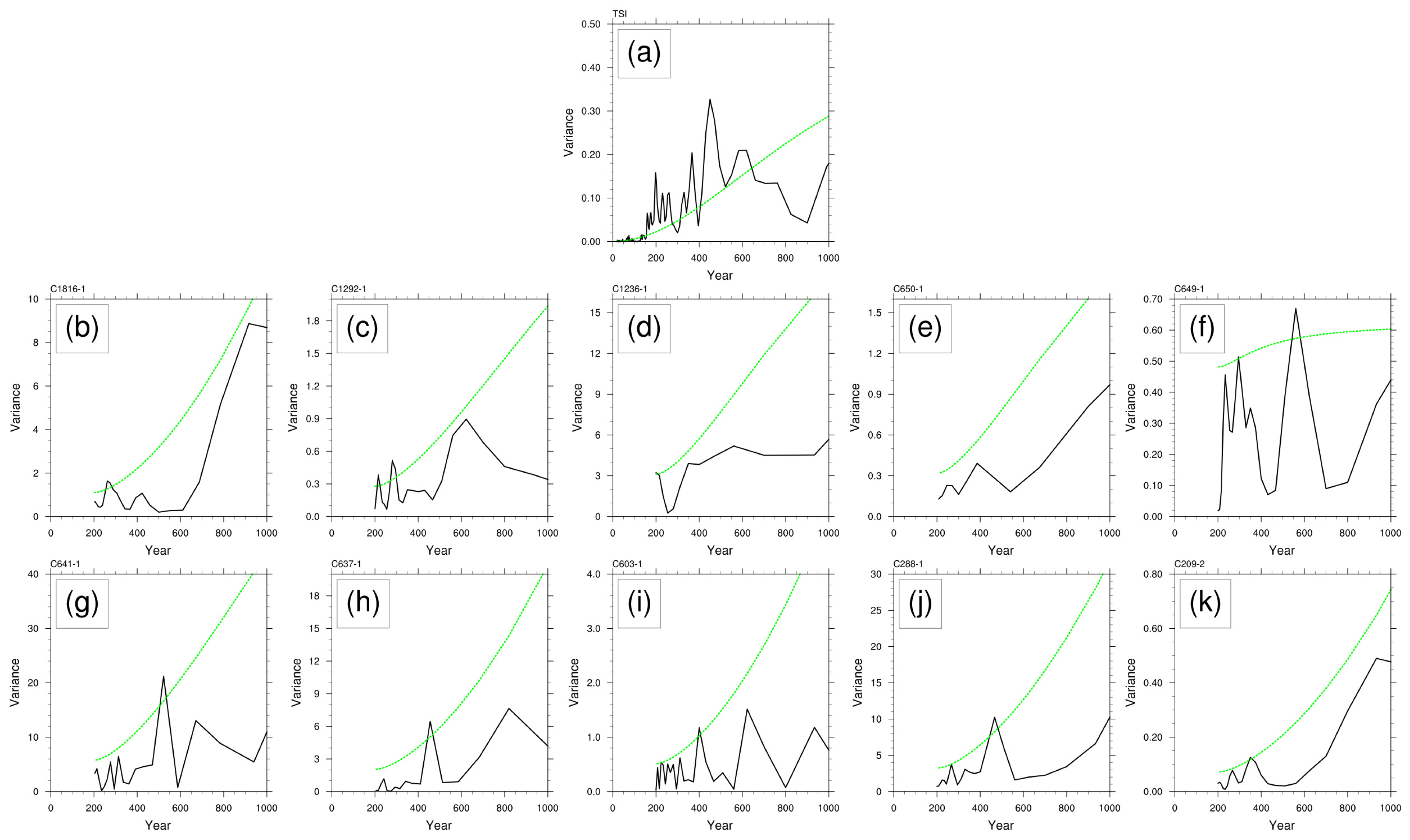
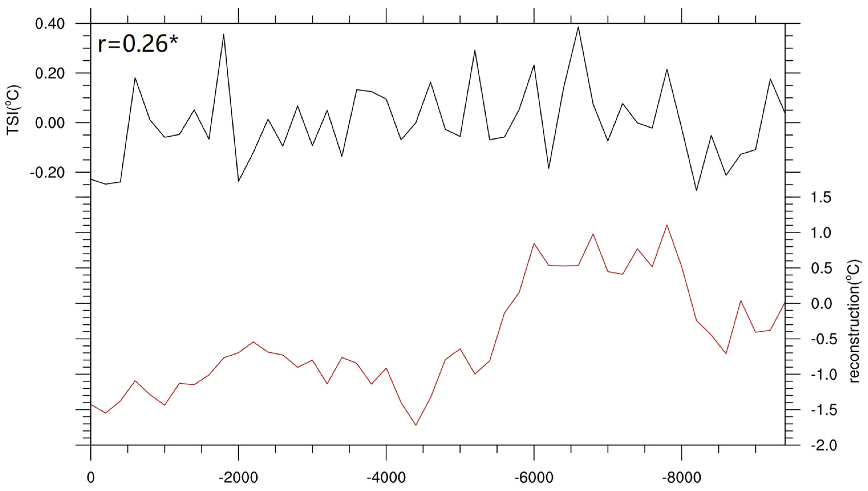
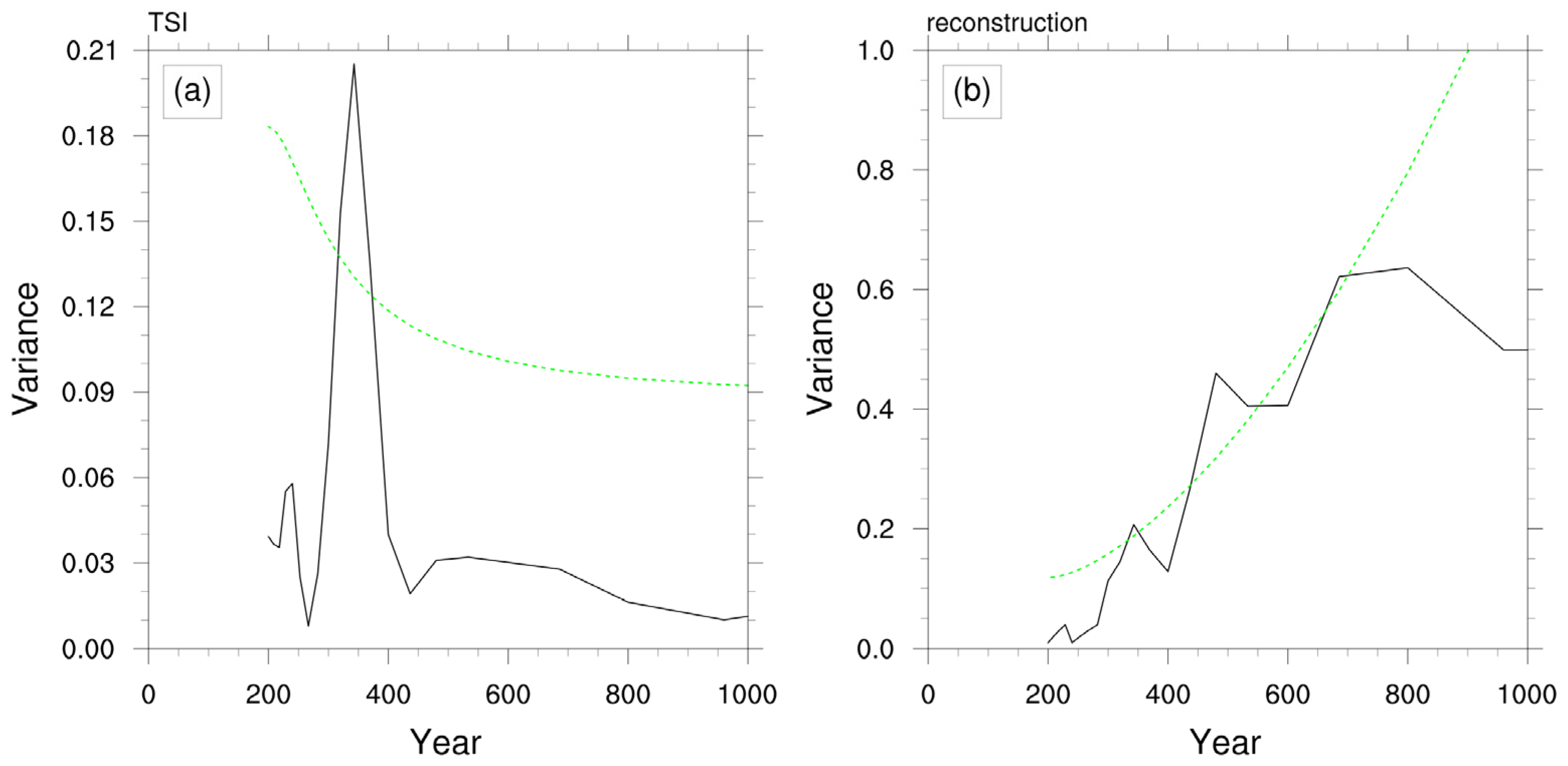
On the one hand, the reconstruction data lacks records of the highest monthly temperature in summer; on the other hand, the time resolution of the reconstruction data is 200 years, so we mainly compared the temporal variation characteristics of summer temperatures on a century scale during the Holocene. To ensure consistency in temporal resolution between TSI and reconstructed data, we conducted an 11-year running average of TSI data. Figure 5 shows the time series of average summer temperature anomaly in China during the Holocene, we found that both in TSI and in reconstructed data, the summer temperatures exhibit significant warm period on centennial time scale. By analyzing the power spectrum (Figure 6), we can find that although no centenary period was found in the C1236-1 and C650-1 data, TSI and other reconstructed data can reflect different centenary periods at a 90% confidence level. Furthermore, in order to better compare TSI data and reconstruction data, we averaged reconstruction data from different regions in China to obtain reconstruction data over the whole China (reconstruction-mean). Due to the time resolution of the reconstruction-mean data is 200 years, there are a total of 48 data in the reconstruction-mean data from 9400 BC to 0 BC. We selected 48 data corresponding to the reconstruction-mean data from the TSI data. The time series (Figure 7) and the power spectrum (Figure 8) of average summer temperature anomalies in China during the Holocene show that there is a significant correlation between the time series of reconstruction-mean and TSI with a correlation coefficient of 0.26 at the 90% confidence level, and these two data can reflect same centenary periods (300–400 years) at a 95% confidence level. In summary, we believe that the TSI data is suitable for studying the spatio-temporal variation of the extreme high temperatures in summer over China.

3.2. Characteristics

The CTRL experiment is driven by the real situation of 1850 AD as a fixed external force which can reflect the internal variability process of the climate system. By comparing the TSI experiment and CTRL experiment, the modulation effect of total solar irradiance forces on climate can be reflected. In this chapter, the EOF1 of the summer extreme temperature over China during the Holocene in the TSI experiment is compared with the EOF1 in the CTRL experiment, respectively, in order to analyze the modulation effect of total solar irradiance forces on the centennial spatial and temporal variation. In order to focus on the centennial time scale, we conducted an 11-year running average of the CTRL and TSI data.
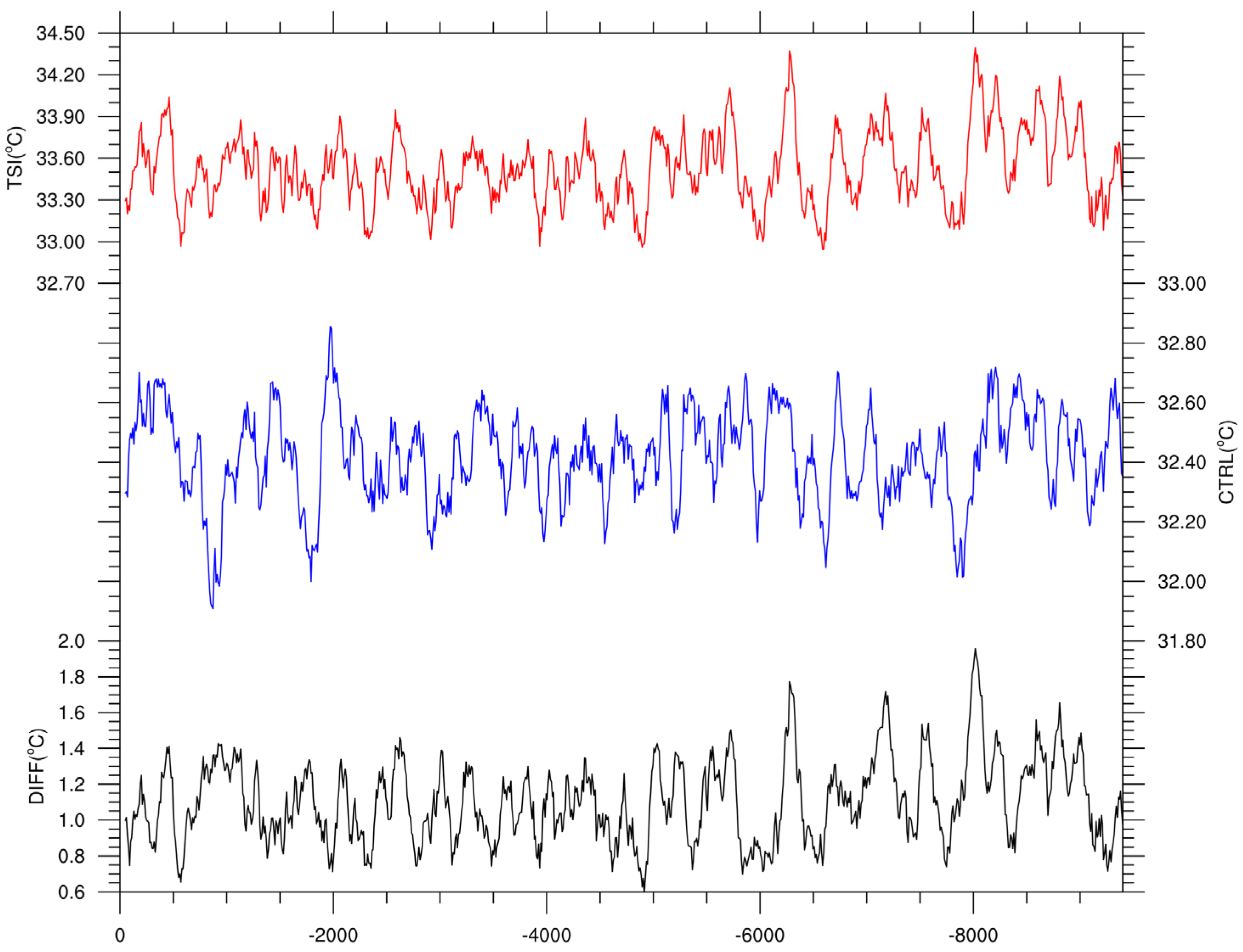
First, we quantitatively distinguished the spatial-temporal distribution characteristics of the average extreme high temperatures in summer over China during Holocene on the centennial time scale. From the spatial distribution of summer extreme high-temperature differences (Figure 9c), we found that compared with the summer extreme high temperatures in the CTRL experiment, the summer extreme high temperatures in the TSI experiment over northeast China is significantly enhanced, with an increase of about 1 °C. Therefore, we believe that under the influence of total solar irradiance, the summer extreme high temperature in northeast China is significantly enhanced. Summer extreme high temperature after the regional average also shows that under the influence of total solar irradiance, the summer extreme high temperature over China is significantly enhanced, with an increase of about 0.6–2.0 °C (Figure 10).
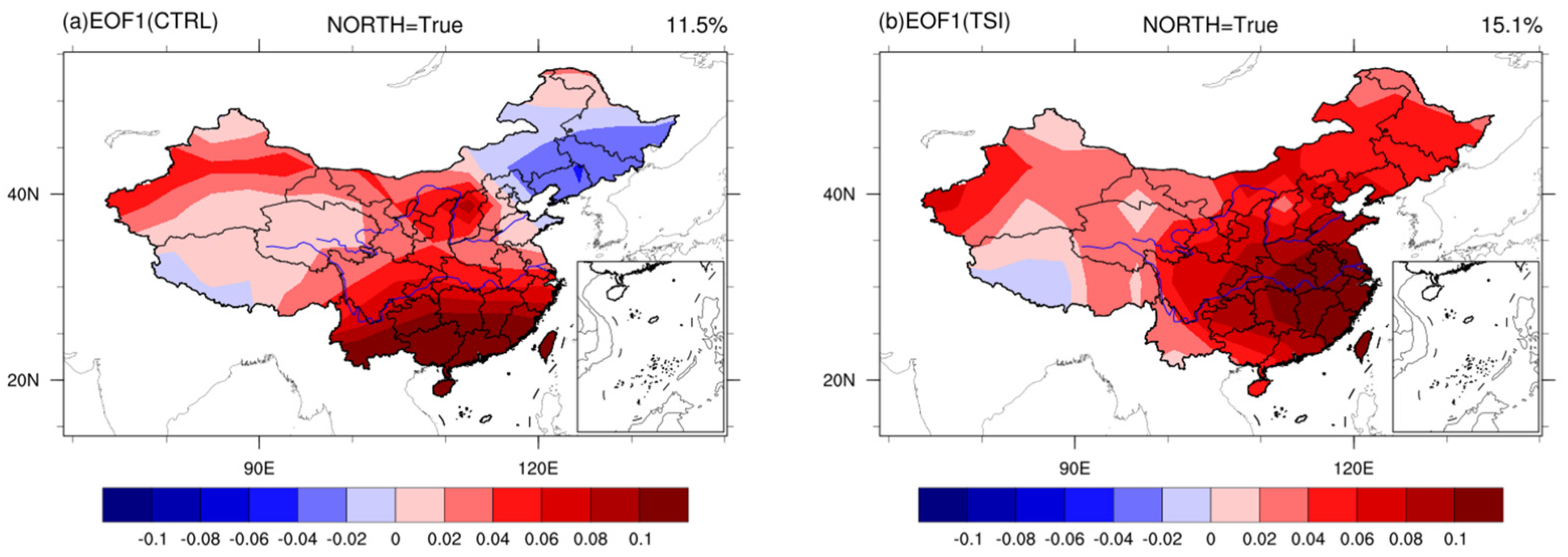
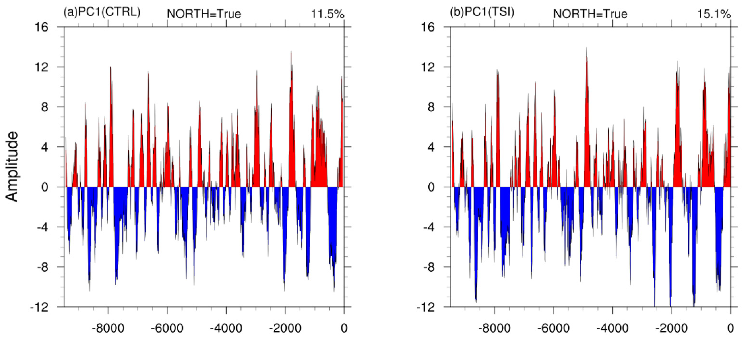
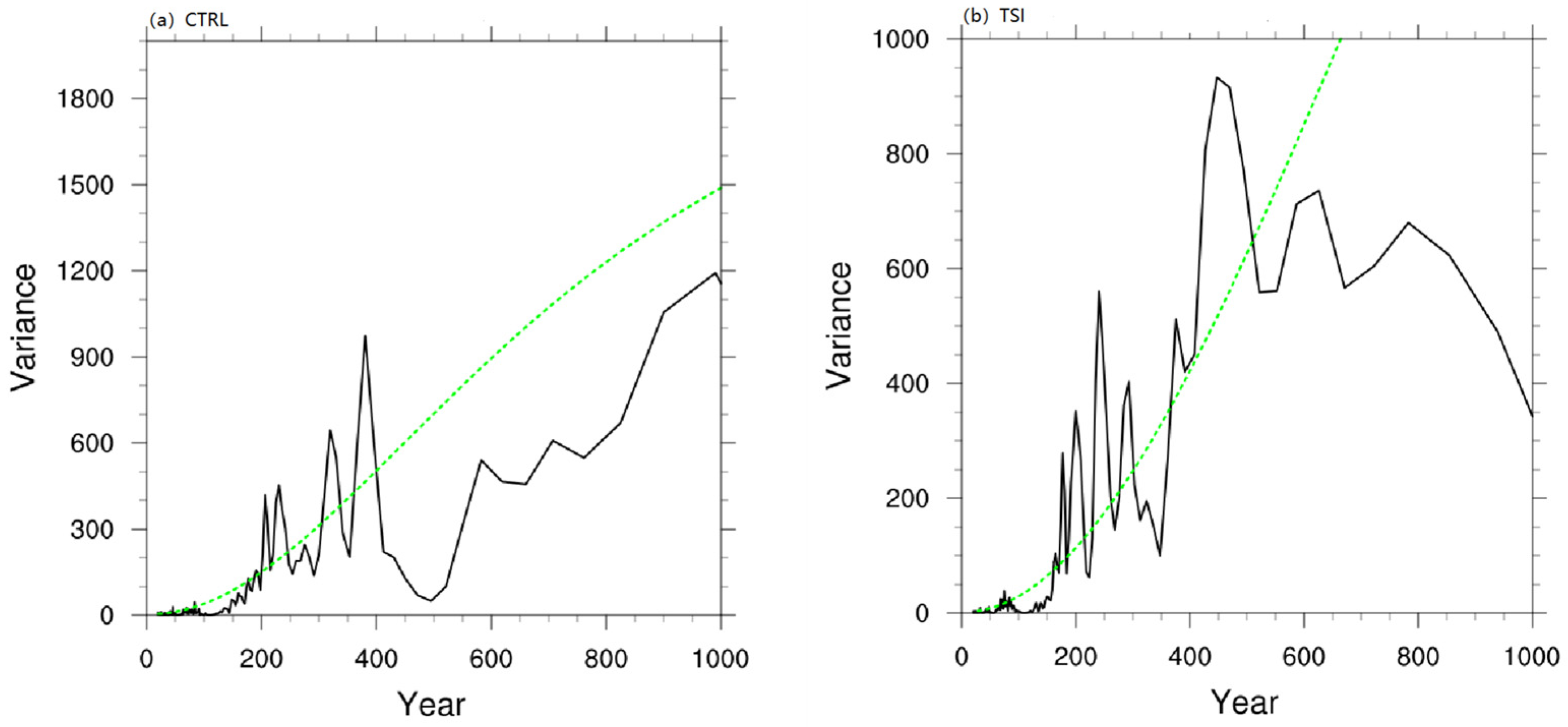
The EOF1, PC1, and power spectrum of PC1 about the extreme high temperatures in summer over China in CTRL during the Holocene are shown in Figure 11a, Figure 12a and Figure 13a. Figure 11a shows the EOF1, with 11.5% of the explained variance and the true result about the North test. It can be seen from EOF1 that the summer extreme high temperature in Northeast China and other regions showed a negative–positive dipole distribution mode. Figure 13a shows the power spectrum of the PC1. It has a clear 200-year and 400-year periodicity at the 95%. However, the summer extreme high temperatures showed different characteristics in TSI experiments (Figure 11b, Figure 12b and Figure 13b). From Figure 11b, it can be seen that in the TSI, the summer extreme high temperature over the whole of China showed a positive distribution mode. Under the regulation of total solar irradiance, there are not only 200-year and 400-year periodicity but also significant 300-year and 500-year periodicity (p < 0.05) (Figure 13b). The result of the North test of EOF1 is true. At the same time, the result of the North test of EOF2 is False. So, we believe that the EOF1 can represent the variation characteristics of extreme high temperatures, although the explained variance of EOF1 is only about 15%.

3.3. Physical Mechanisms

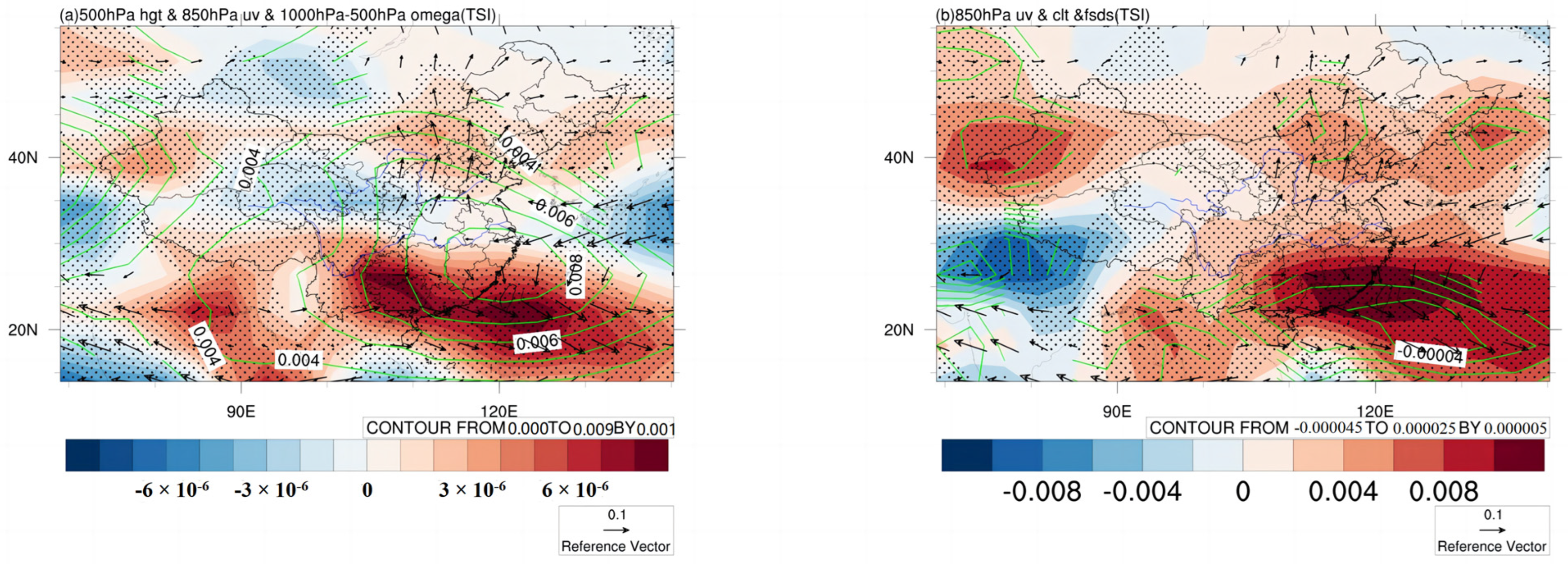
By using the regression analysis method, the physical mechanisms of the spatial and temporal variation characteristics of the extreme high temperatures in summer over China during the Holocene in the CTRL experiment and TSI experiment were discussed through the analysis of 500 hPa geopotential height, 1000–500 hPa vertical velocity, 850 hPa wind, total cloud cover, and downward solar flux.
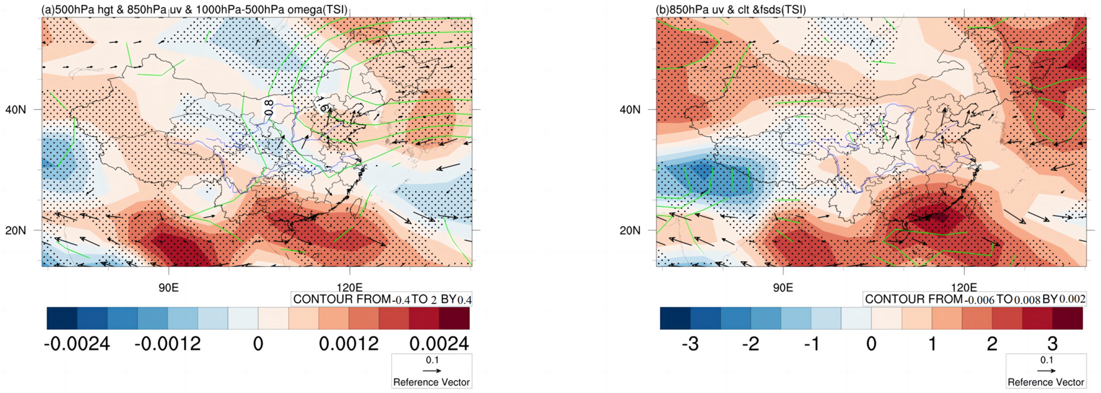
Figure 14 shows the regression coefficient of 500 hPa geopotential height (Figure 14a), 850 hPa wind (Figure 14a), 1000–500 hPa vertical velocity (Figure 14a), total cloud cover (Figure 14b), and downward solar flux (Figure 14b) of the extreme high temperature in summer over China during the Holocene in the TSI experiment to PC1 (TSI). The regression coefficient distribution shows that there is an obvious high geopotential height anomaly over Northeast China, which is conducive to the summer extreme high temperatures. The regression distribution of wind shows that there are obvious anticyclones in Northeast China, which is conducive to the rise of local temperatures. The regression distribution of vertical velocity indicates that there are positive values in Northeast China, representing downward movement. The downward movement of vertical velocity is conducive to an increase in temperature. The regression distribution of total cloud cover indicates that there are negative values in Northeast China, representing a decrease in total cloud cover. A decrease in total cloud cover is conducive to an increase in temperature. The regression distribution of downward solar flux indicates that in Northeast China, the values are positive, indicating an increase in downward solar flux. An increase in downward solar flux is conducive to an increase in temperature. In summary, the results show that all regions of China, including Northeast China, have shown significant high pressure. The anticyclone under high pressure will lead to obvious subsidence movement and a decrease of the total cloud layer, which will lead to the increase of downward solar radiant flux and further increase of the highest temperature in summer. To sum up, we found that under the influence of solar radiation, there was a circulation field in northeast China that was conducive to the occurrence of the extreme high temperature in summer during the Holocene.
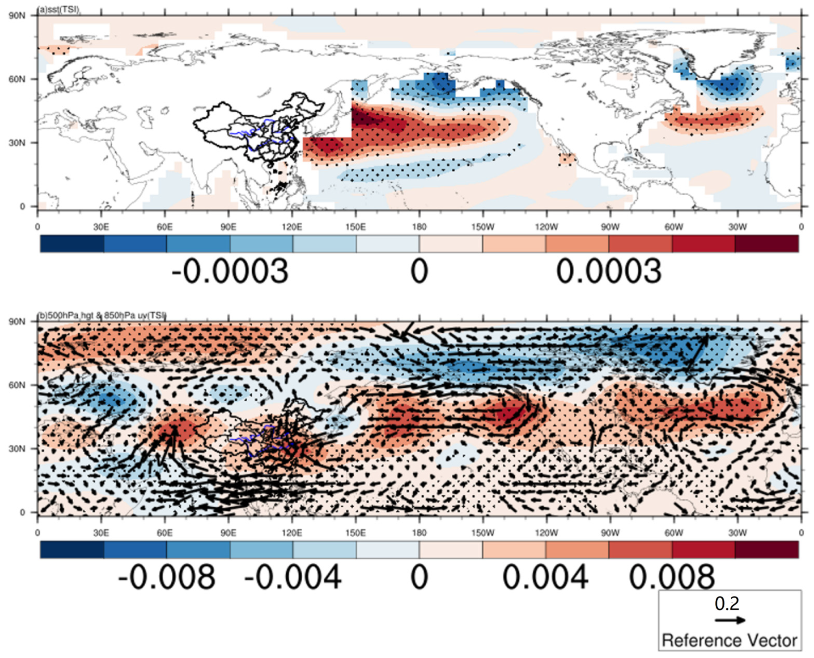
In TSI, the formation of this anticyclonic anomaly over Northeast China could be further attributed to the SST anomalies over the Northwest Pacific and an upper-tropospheric wave train in the mid-to-high latitudes (Figure 15). On one hand, associated with the summer extreme high temperature, the SST anomaly over the Northwest Pacific feature a PDO pattern, which could enhance the anticyclone in the northwest Pacific and influence the Northeast China (Figure 15b). On the other hand, the most prominent characteristic of the summer extreme high-temperature-related upper-level circulation is a Rossby wave train with a barotropic structure consisting of successive pressure ridges from Eurasia to North America and the North Atlantic, which is similar to the circum-global teleconnection found by Ding and Wang (2005) [47] (Figure 15b). The positive centers of this wave train are located over West Asia, East Asia, the North Pacific, North America, and the North Atlantic, contributing to the formation of a low-level anticyclonic anomaly over the Northeast China.
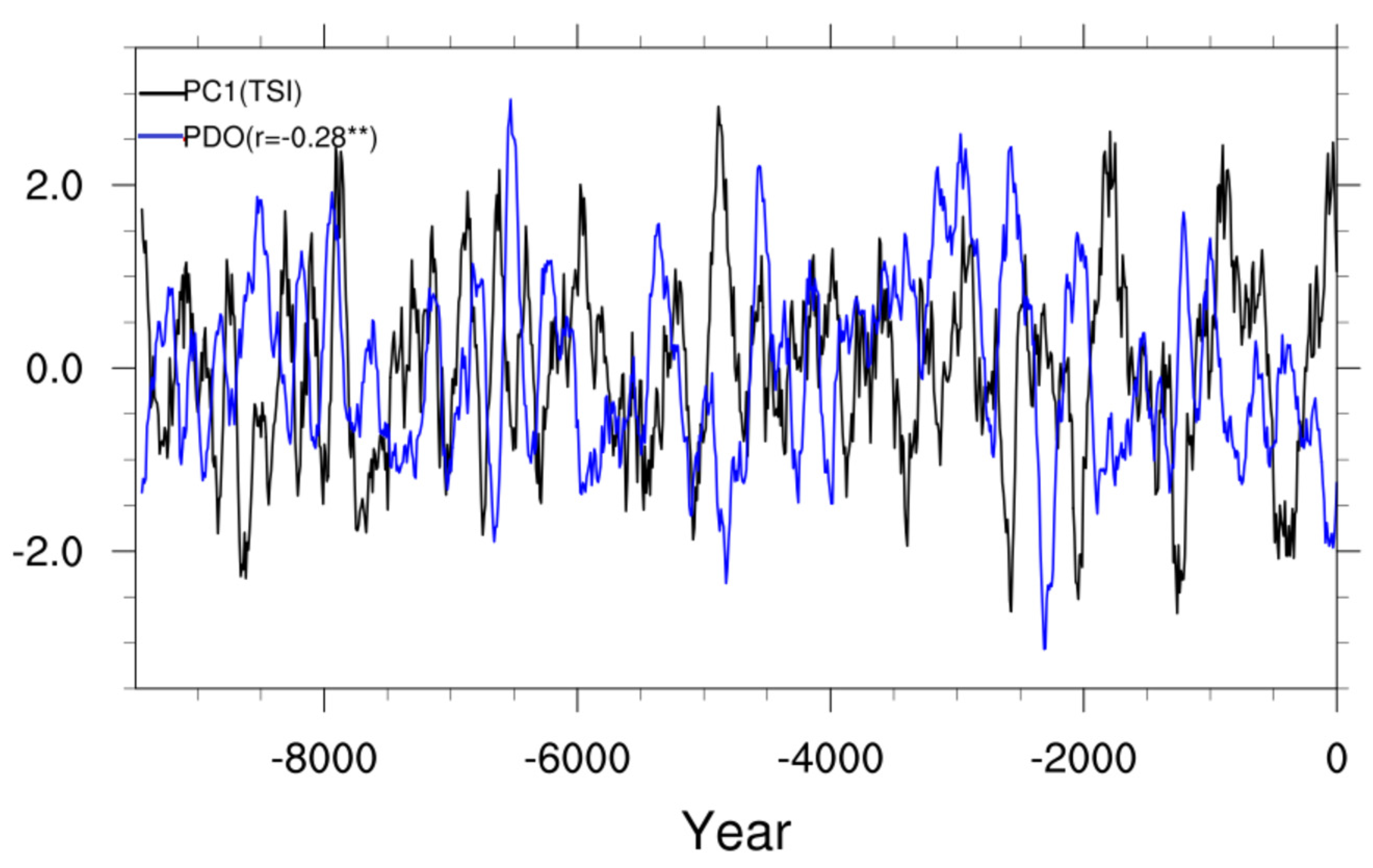
Finally, we preliminarily explored the underlying physical mechanism through which total solar irradiance variation on affects the atmospheric circulation pattern and their impact on regional summer extreme high temperatures. From Figure 15a, we can find that the SST anomaly over the Northwest Pacific feature a PDO pattern, so we calculated the correlation between PCI and PDO in the TSI experiment (Figure 16). Not only did we find that there is a clear correlation between PCI and PDO with a correlation coefficient of 0.28 at the 95% confidence level, but also we found that PDO appear centennial cycles of 200 years, 300 years, 400 years, and 500 years, similar to PC1 (Figure 17b). Like that, does the external forcing sequence used in TSI experiments also have the same centennial cycles? The power spectrum analysis result (Figure 17a) shows that the same centennial cycles can be found in the external forcing sequence. Therefore, we conjecture that the centennial variation of total solar irradiance leads to the centennial variation of PDO, and further affects the centennial variation of summer extreme high temperatures in northeast China.
Figure 18 shows the regression coefficient of 500 hPa geopotential height (Figure 18a), 850 hPa wind (Figure 18a), 1000–500 hPa vertical velocity (Figure 18a), total cloud cover (Figure 18b), and downward solar flux (Figure 14b) of the extreme high temperatures in summer over China during the Holocene in TSI experiment to PDO (TSI). The regression coefficient distribution shows that there is an obvious high geopotential height anomaly, obvious anticyclones, downward movement, a decrease in total cloud cover, and an increase in downward solar flux in northeast China. To sum up, under the influence of PDO, the obvious subsidence movement and the increase of downward solar radiant flux further increase the summer extreme highest temperature in northeast China.

4. Discussion

There are still some problems in this research:
1. Comparison with reconstruction data. Because there is no integrated reconstruction data of the highest temperature in summer over China during the Holocene at present, only the reconstruction data of summer average temperatures were compared when the model simulation capability was verified, so the comparison between simulation and reconstruction data needs to be further strengthened;
2. Uncertainty of simulation analysis. Although several experiments are used for comparison, each experiment is only run once, which may have some uncertainty. Therefore, averaging the results of multiple experiments and integrating the results of multiple models need to be further developed. Including outputs from multiple climate models could help to assess the robustness and consistency of the results;
3. In this paper, we only focus on the impact of total solar irradiance on the centennial variation of extreme high temperatures. Exploring the influence of other factors such as greenhouse gas emissions, land-use changes, and aerosol effects could provide a more comprehensive understanding of the drivers of extreme temperature variations;
4. We only focus on the centennial variation of extreme high temperatures, Expanding the temporal scope beyond the Holocene period, such as examining longer geological timescales, may offer valuable insights into the long-term trends and variability associated with solar forcing.

5. Conclusions

In this paper, the variation and mechanism of the extreme high temperatures in summer over China during the Holocene on the centennial scale experiment forced by total solar irradiance are analyzed. The results show that:
1. The TSI experiment is relatively reliable in simulating the summer extreme high temperature over China during the Holocene. Under the modulation of total solar irradiance, the centennial spatial pattern changed from dipole mode to uniform mode, the difference being that the mode in northeast China changed from negative to positive. At the same time, there were obvious periodicity of 300-year and 500-year;
2. Under the influence of total solar irradiance, it shows significant high pressure in northeast China. The anticyclone under high pressure will lead to obvious subsidence movement and a decrease of the total cloud layer, which will lead to the increase of downward solar radiant flux and further increase of the summer extreme high temperatures;
3. Under the influence of total solar irradiance, the center of the Rossby wave train in the barotropic structure of the upper circulation related to the summer extreme high temperatures significantly moves northward. This barotropic structure is composed of continuous pressure ridges from Eurasia to North America and the North Atlantic, which is conducive to the increase of the summer extreme high temperature in Northeast China;
4. We conjecture that the centennial variation of total solar irradiance leads to the centennial variation of PDO, and further affects the centennial variation of summer extreme high temperatures in northeast China. PDO leads to obvious subsidence movement and an increase in radiation flux, causing an increase in extreme high temperatures over northeast China.
This study examines the characteristics and physical mechanisms of extreme high temperatures in summer in China during the Holocene period. Present research sheds light on the important influence of solar activity on these temperature variations and provides valuable insights for predicting future extreme climate events. The shift from a dipole mode to a uniform mode, along with the observed periodicities of 300 years and 500 years, highlights the significance of solar irradiance in shaping the centennial-scale characteristics of extremely high temperatures. This discovery enhances our understanding of the complex interplay between solar activity and climate dynamics.

Author Contributions

Conceptualization, L.L., W.S. and J.L.; methodology, L.L., W.S. and J.L.; formal analysis, L.L.; data curation, L.L., J.L. and L.W.; writing—original draft preparation, L.L.; writing—review and editing, W.S., J.L. and L.W.; visualization, L.L.; supervision, W.S. and J.L.; funding acquisition, J.L. All authors have read and agreed to the published version of the manuscript.

Funding

This research was funded by the National Natural Science Foundation of China (Grant Nos. 42130604, 42105044, 41971108, and 42111530182), the Priority Academic Development Program of Jiangsu Higher Education Institutions (Grant No. 164320H116), and the Fundamental Research Funds for the Central Universities (202362001, 202072010).

Data Availability Statement

The data presented in this study are available on request from the corresponding author.

Conflicts of Interest

The authors declare no conflict of interest.

References

  1. Easterling, D.R.; Meehl, G.A.; Parmesan, C.; Changnon, S.A.; Karl, T.R.; Mearns, L.O. Climate extremes: Observations, modeling, and impacts. Science 2000, 289, 2068–2074. [Google Scholar] [PubMed] [Green Version]
  2. Meehl, G.A.; Tebaldi, C. More intense, more frequent, and longer lasting heat waves in the 21st century. Science 2004, 305, 994. [Google Scholar] [CrossRef] [PubMed] [Green Version]
  3. IPCC. Climate Change 2021: The Physical Science Basis [M/OL]. 2021. Available online: https://www.ipcc.ch/report/ar6/wg1/downloads/report/IPCC_AR6_WGI_Full_Report.pdf (accessed on 24 June 2023).
  4. Ge, Q.; Liu, J.; Fang, X.; Yang, B.; Hao, Z.; Shao, X.; Zheng, J. General characteristics of temperature change and centennial warm periods during the past 2000 years. Acta Geogr. Sin. 2013, 68, 579–592. [Google Scholar]
  5. IPCC. Climate Change 2013: The Physical Science Basis [M/OL]; In Press; Cambridge University Press: Cambridge, UK, 2013; Available online: https://www.ipcc.ch/report/ar5/wg1/ (accessed on 24 June 2023).
  6. Dahe, Q.; Stocker, T. Highlights of the IPCC Working Group I Fifth Assessment Report. Clim. Chang. Res. 2014, 10, 1. [Google Scholar]
  7. Marcott, S.A.; Shakun, J.D.; Clark, P.U.; Mix, A.C. A reconstruction of regional and global temperature for the past 11,300 years. Science 2013, 399, 1198–1201. [Google Scholar] [CrossRef] [Green Version]
  8. Fang, X.; Hou, G. Synthetically reconstructed Holocene temperature change in China. Sci. Geogr. Sin. 2011, 31, 385–393. [Google Scholar]
  9. Wu, H.; Li, Q.; Yu, Y.; Jiang, W.; Lin, Y.; Sun, A.; Luo, Y. Quantitative climate reconstruction in China during the mid-Holocene. Quat. Sci. 2017, 37, 982–998. [Google Scholar] [CrossRef]
  10. Xiaoying, P.; Wei, Z.; Yinjuan, Z. Preliminary research in the Holocene Hypsithermal climate change. J. S. China Norm. Univ. Nat. Sci. Ed. 2005, 2, 52–60. [Google Scholar]
  11. Wang, S.; Gong, D. The temperature of China in several characteristic periods of the Holocene. Prog. Nat. Sci. 2000, 10, 325–332. (In Chinese) [Google Scholar]
  12. Ge, Q.; Wang, S.; Zheng, J. Reconstruction of China’s temperature change sequence in the past 5000 years. Prog. Nat. Sci. 2006, 16, 689–696. (In Chinese) [Google Scholar]
  13. Hou, G.; Fang, X. Characteristics of Holocene Temperature Change in China. Prog. Geogr. 2011, 30, 1075–1080. [Google Scholar]
  14. Chen, X.; Xu, Y.; Xu, C.; Yao, Y. Assessment of Precipitation Simulations in China by CMIP5 Multi-models. Clim. Chang. Res. 2014, 10, 217–225. [Google Scholar]
  15. Taylor, K.E.; Stouffer, R.J.; Meehl, G.A. An overview of CMIP5 and the experiment design. Bull. Am. Meteorol. Soc. 2012, 93, 485–498. [Google Scholar] [CrossRef] [Green Version]
  16. Jiang, D.; Tian, Z. Last Glacial Maximum and mid-Holocene water vapor transport over East Asia: A modeling study. Quat. Sci. 2017, 37, 999–1008. [Google Scholar] [CrossRef]
  17. Wang, Z.; Wang, J.; Zhang, S.; Li, K.; Zuo, R.; Liu, J. Impact of different timescales on the characteristics and mechanisms of the Northern Hemisphere Summer Monsoon: Based on the CESM results. Quat. Sci. 2018, 38, 1494–1506. [Google Scholar] [CrossRef]
  18. Ren, X.; Shi, Z.G. Response of global temperature extremes in mid-Holocene: Results from MPI-ESM-P experiments. J. Earth Environ. 2019, 10, 465–478. [Google Scholar]
  19. He, F. Simulating Transient Climate Evolution of the Last deglaciation with CCSM3, Doctor of Philosophy, Atmospheric and Oceanic Sciences; University of Wisconsin: Madison, WI, USA, 2011; p. 161. [Google Scholar]
  20. Yan, M.; Liu, J. Physical processes of cooling and mega-drought during the 4.2 ka bp event: Results from trace-21 ka simulations. Clim. Past 2019, 15, 265–277. [Google Scholar] [CrossRef] [Green Version]
  21. Morrill, C.; Overpeck, J.T.; Cole, J.E. A synthesis of abrupt changes in the Asian summer monsoon since the last deglaciation. Holocene 2003, 13, 465–476. [Google Scholar] [CrossRef]
  22. Berkelhammer, M.; Sinha, A.; Mudelsee, M.; Cheng, G.D.; Edwards, R.L.; Cannariato, K. Persistent multidecadal power of the Indian Summer Monsoon. Earth Planet. Sci. Lett. 2010, 290, 166–172. [Google Scholar] [CrossRef]
  23. Fleitmann, D.; Burns, S.J.; Mudelsee, M.; Neff, U.; Kramers, J.; Mangini, A.; Matter, A. Holocene forcing of the Indian monsoon recorded in a stalagmite from Southern Oman. Science 2003, 300, 1737–1739. [Google Scholar] [CrossRef] [Green Version]
  24. Wang, Y.J.; Cheng, H.; Edwards, R.L.; He, Y.Q.; Kong, X.G.; An, Z.S.; Wu, J.Y.; Kelly, M.J.; Dykoski, C.A.; Li, X.D. The Holocene Asian monsoon: Links to solar changes and North Atlantic climate. Science 2005, 308, 854–857. [Google Scholar] [CrossRef]
  25. Knudsen, M.F.; Seidenkrantz, M.-S.; Jacobsen, B.H.; Kuijpers, A. Tracking the Atlantic Multidecadal Oscillation through the last 8000 years. Nat. Commun. 2011, 2, 178. [Google Scholar] [CrossRef] [Green Version]
  26. Feng, S.; Hu, Q.; Oglesby, R.J. AMO-like variations of Holocene sea surface temperatures in the North Atlantic Ocean. Clim. Past Discuss. 2009, 5, 2465–2496. [Google Scholar]
  27. Conroy, J.L.; Hudson, A.M.; Overpeck, J.T.; Liu, K.B. The primacy of multidecadal to centennial variability over late-Holocene forced change of the Asian Monsoon on the southern Tibetan Plateau. Earth Planet. Sci. Lett. 2017, 458, 337–348. [Google Scholar] [CrossRef] [Green Version]
  28. Tan, L.; Cai, Y.; An, Z.; Cheng, H.; Yi, L.; Lawrence Edwards, R. High-resolution monsoon precipitation variations in southern Shaanxi, Central China during 4200~2000 a B.P. as revealed by speleothem δ18O and Sr/Ca records. Quat. Sci. 2014, 34, 1238–1245. [Google Scholar] [CrossRef]
  29. Herschel, W. Observations tending to investigate the nature of the sun, in order to find the causes or symptoms of its variable emission of light and heat; with remarks on the use that may possibly be drawn from solar observations. Proc. R. Soc. Lond. 1801, 91, 265–318. [Google Scholar]
  30. Laut, P.; Gundermann, J. Solar cycle length hypothesis appears to support the ipcc on global warming. J. Atmos. Sol. Terr. Phys. 1999, 60, 1719–1728. [Google Scholar] [CrossRef]
  31. Tung, K.K.; Camp, C.D. Solar cycle warming at the Earth’s surface in NCEP and ERA-40 data: A linear discriminant analysis. J. Geophys. Res. Atmos. 2008, 113, 1–11. [Google Scholar] [CrossRef] [Green Version]
  32. Haigh, J.D. The Impact of Solar Variability on Climate. Science 1996, 272, 981–984. [Google Scholar] [CrossRef]
  33. Meehl, G.A.; Arblaster, J.M.; Matthes, K.; Sassi, F.; van Loon, H. Amplifying the Pacific climate system response to a small 11-year solar cycle forcing. Science 2009, 325, 1114–1118. [Google Scholar] [CrossRef] [Green Version]
  34. Wang, B.; Zhou, T.; Yu, Y. A perspective on Earth system model development. Acta Meteorol. Sin. 2008, 66, 857–869. [Google Scholar] [CrossRef]
  35. Zheng, P.; Song, J.; Zhang, F.; Bao, X. Common instruction of some OGCM. Mar. Forecast. 2008, 25, 108–120. [Google Scholar] [CrossRef]
  36. Vieira LE, A.; Solanki, S.K.; Krivova, N.A.; Usoskin, I. Evolution of the solar irradiance during the Holocene. Astron. Astrophys. 2011, 531, A6. [Google Scholar] [CrossRef] [Green Version]
  37. Stebich, M.; Rehfeld, K.; Schlütz, F.; Tarasov, P.E. Corrigendum to “Holocene vegetation and climate dynamics of NE China based on the pollen record from Sihailongwan Maar Lake”. Quat. Sci. Rev. 2015, 124, 275–289. [Google Scholar] [CrossRef] [Green Version]
  38. Herzschuh, U.; Kramer, A.; Mischke, S.; Zhang, C. Quantitative climate and vegetation trends since the late glacial on the northeastern Tibetan Plateau deduced from Koucha Lake pollen spectra. Quat. Res. 2009, 71, 162–171. [Google Scholar] [CrossRef]
  39. Yu, S.-Y. Quantitative reconstruction of mid- to late-Holocene climate in NE China from peat cellulose stable oxygen and carbon isotope records and mechanistic models. Holocene 2013, 11, 1507–1516. [Google Scholar] [CrossRef]
  40. Chang, J.; Zhang, E.L.; Liu, E.F.; Shulmeister, J. Summer temperature variability inferred from subfossil chironomid assemblages from the south-east margin of the Qinghai-Tibetan Plateau for the last 5000 years. Holocene 2017, 27, 1876–1884. [Google Scholar] [CrossRef]
  41. Zhang, E.; Chang, J.; Cao, Y.; Sun, W.; Shulmeister, J. Holocene high-resolution quantitative summer temperature reconstruction based on subfossil chironomids from the southeast margin of the Qinghai-Tibetan Plateau. Quat. Sci. Rev. 2017, 165, 1–12. [Google Scholar] [CrossRef]
  42. Zhao, J.; An, C.B.; Huang, Y.; Morrill, C.; Chen, F.H. Contrasting early Holocene temperature variations between monsoonal East Asia and westerly dominated Central Asia. Quat. Sci. Rev. 2017, 178, 14–23. [Google Scholar]
  43. Zhao, C.; Liu, Z.; Rohling, E.J.; Yu, Z.; Liu, W.; He, Y.; Zhao, Y.; Chen, F. Holocene temperature fluctuations in the northern Tibetan Plateau. Quat. Res. 2013, 80, 55–65. [Google Scholar] [CrossRef]
  44. Wu, D.; Chen, X.; Lv, F.; Brenner, M.; Curtis, J.; Zhou, A. Decoupled early Holocene summer temperature and monsoon precipitation in southwest China. Quat. Sci. Rev. 2018, 193, 54–67. [Google Scholar] [CrossRef]
  45. Hou, J.H.J.; Huang, Y.H.Y.; Zhao, J.Z.J.; Liu, Z.; Colman, S.; An, Z. Large Holocene summer temperature oscillations and impact on the peopling of the northeastern Tibetan Plateau. Geophys. Res. Lett. 2016, 43, 1323–1330. [Google Scholar] [CrossRef] [Green Version]
  46. Wen, R.L.; Xiao, J.L.; Chang, Z.G.; Zhai, D.Y.; Xu, Q.H.; Li, Y.C.; Itoh, S. Holocene precipitation and temperature variations in the East Asian monsoonal margin from pollen data from Hulun Lake in northeastern Inner Mongolia, China. Boreas 2010, 39, 262–272. [Google Scholar] [CrossRef]
  47. Ding, Q.H.; Wang, B. Circumglobal teleconnection in the Northern Hemisphere summer. J. Clim. 2005, 18, 3483–3505. [Google Scholar] [CrossRef]
Figure 1. The location of the reconstruction data. Red point: whole Holocene. Blue point: a certain period of Holocene.
Atmosphere 14 01207 g001
Figure 2. Spatial distribution of the extreme high temperature in summer over China from 1950 to 1990. (a) NCEP1 (b) TSI unit: °C. ** 95% confidence level. r-spatial correlation coefficient. The degree of freedom is 27.
Atmosphere 14 01207 g002
Figure 3. Spatial distribution of the extreme high temperatures in summer over China from 1851 to 1990. (a) 20CR (b) TSI unit: °C. ** 95% confidence level. r-spatial correlation coefficient. The degree of freedom is 36.
Atmosphere 14 01207 g003
Figure 4. Time series of the extreme high temperatures in summer over China from 1851 to 1990. Red line: 20CR. Black line: TSI. unit: °C. ** 95% confidence level. r-temporal correlation coefficient. The degree of freedom is 13.
Atmosphere 14 01207 g004
Figure 5. Time series of average summer temperature anomaly over China during the Holocene. unit: °C. Black line: TSI. Brown line:C1816-1. Green line: C1292-1. Orange line: C1236-1. Red line: C650-1. Blue line: C649-1. Yellow Line: C641-1. Purple line: C637-1. Cyan line: C603-1. Pink line: C288-1. Deep pink line: C209-2. Grey line: average.
Atmosphere 14 01207 g005
Figure 6. The power spectrum of average summer temperature anomaly over China during the Holocene. (a) TSI (bk) Reconstruction. Green line: 90% confidence level.
Atmosphere 14 01207 g006
Figure 7. Time series of average summer temperature anomaly over China during the Holocene. Red line: Reconstruction. Black line: TSI. Unit: °C. * 90% confidence level. r-temporal correlation coefficient. The degree of freedom is 46.
Atmosphere 14 01207 g007
Figure 8. The power spectrum of average summer temperature anomaly over China during the Holocene. (a) TSI (b) Reconstruction. Green line: 95% confidence level.
Atmosphere 14 01207 g008
Figure 9. The spatial distribution characteristics of the average extreme high temperatures in summer over China during Holocene. (a) CTRL (b) TSI (c) TSI-CTRL. Unit: °C. The different anomalies are significant at the 95% confidence level are shown.
Atmosphere 14 01207 g009
Figure 10. The time series of the average extreme high temperatures in summer over China during Holocene. Red line: TSI. Blue line: CTRL. Black line: TSI-CTRL. Unit: °C.
Atmosphere 14 01207 g010
Figure 11. The EOF1 of the extreme high temperatures in summer over China during the Holocene in CTRL and TSI. (a) CTRL (b) TSI.
Atmosphere 14 01207 g011
Figure 12. The PC1 of the extreme high temperatures in summer in China during the Holocene in CTRL and TSI. (a) CTRL (b) TSI.
Atmosphere 14 01207 g012
Figure 13. The power spectrum of the extreme high temperatures in summer in China during the Holocene in CTRL and TSI. (a) CTRL (b) TSI. Green line: 95% confidence level.
Atmosphere 14 01207 g013
Figure 14. Regression coefficients of 500 hPa geopotential height (a, contour), 850 hPa wind (a, vctor), 1000–500 hPa vertical velocity (a, shading), total cloud cover (b, contour), and downward solar flux (b, shading) to PC1 (TSI) of the extreme high temperatures in summer over China during the Holocene in TSI. The winds anomalies significant at the 95% confidence level are shown. The 500 hPa geopotential height and total cloud cover anomalies significant at the 95% confidence level are shown. Dots indicate the 1000–500 hPa vertical velocity and downward solar flux anomalies significant at the 95% confidence level.
Atmosphere 14 01207 g014
Figure 15. Figure 15. Regression coefficients of sea surface temperature (a), 500 hPa geopotential height (b, shading), and 850 hPa wind (b, vector) to PC1 (TSI) of the highest temperature in summer over China during the Holocene in TSI. The winds anomalies significant at the 95% confidence level are shown. Dots indicate the 500 hPa geopotential height anomalies significant at the 95% confidence level.
Atmosphere 14 01207 g015
Figure 16. Time series of the PC1 of the extreme high temperatures in summer over China during the Holocene and the PDO in TSI. Black line: PC1. Blue line: PDO. ** 95% confidence level. r-temporal correlation coefficient. The degree of freedom is 93.
Atmosphere 14 01207 g016
Figure 17. The power spectrum of the total solar irradiance and PDO in TSI. (a) total solar irradiance (b) PDO. Green line: 95% confidence level.
Atmosphere 14 01207 g017
Figure 18. Regression coefficients of 500 hPa geopotential height (a, contour), 850 hPa wind (a, vctor), 1000–500 hPa vertical velocity (a, shading), total cloud cover (b, contour), and downward solar flux (b, shading) to PDO (TSI) of the extreme high temperatures in summer over China during the Holocene in TSI. The wind anomalies significant at the 95% confidence level are shown. The 500 hPa geopotential height and total cloud cover anomalies significant at the 95% confidence level are shown. Dots indicate the 1000–500 hPa vertical velocity and downward solar flux anomalies significant at the 95% confidence level.
Atmosphere 14 01207 g018
Table 1. NNU_Hol experiments.
Experiment NameAbbreviationSpatial ResolutionTime ResolutionTime
Control experimentCTRL3.75° × 3.75°10a10,000 BC–1990 AD
Orbital experimentORB3.75° × 3.75°10a10,000 BC–1990 AD
Total solar irradiance and Orbital experimentTSI_ORB3.75° × 3.75°10a9490 BC–1990 AD
Table 2. Reconstruction data.
IDLon & LatTime ResolutionSeasonTimeReference
C1816-1E 126.6, N 42.28200asummer11,000 BC–200 BCStebich M et al. (2015) [37]
C1292-1E 97.2, N 34200asummer11,000 BC–0 BCHerzschuh U et al. (2009) [38]
C1236-1E 126.37, N 42.33200asummer5600 BC–200 BCShi-Yong Yu, (2013) [39]
C650-1E 100.07, N 27.36200asummer5200 BC–0 BCJie Chang et al. (2017) [40]
C649-1E 99.72, N 26.63200asummer11,000 BC–0 BCZhang E et al. (2017) [41]
C641-1 E 92.8, N 43.66200asummer11,000 BC–1800 BCJiaju Zhao et al. (2017) [42]
C637-1E 96.91, N 37.28200asummer8600 BC–600 BCCheng Zhao et al. (2013) [43]
C603-1E 102.79, N 24.34200asummer11,000 BC–0 BCWu D et al. (2018) [44]
C288-1E 100.14, N 36.81200asummer11,000 BC–0 BCJuzhi Hou et al. (2016) [45]
C209-2E 117.5, N 49.13200asummer11,000 BC–0 BCWen R.L. et al. (2010) [46]
Disclaimer/Publisher’s Note: The statements, opinions and data contained in all publications are solely those of the individual author(s) and contributor(s) and not of MDPI and/or the editor(s). MDPI and/or the editor(s) disclaim responsibility for any injury to people or property resulting from any ideas, methods, instructions or products referred to in the content.