PM_2.5 Concentration Forecasting Using Weighted Bi-LSTM and Random Forest Feature Importance-Based Feature Selection

Abstract

Particulate matter (PM) in the air can cause various health problems and diseases in humans. In particular, the smaller size of PM${}_{2.5}$ enable them to penetrate deep into the lungs, causing severe health impacts. Exposure to PM${}_{2.5}$ can result in respiratory, cardiovascular, and allergic diseases, and prolonged exposure has also been linked to an increased risk of cancer, including lung cancer. Therefore, forecasting the PM${}_{2.5}$ concentration in the surrounding is crucial for preventing these adverse health effects. This paper proposes a method for forecasting the PM${}_{2.5}$ concentration after 1 h using bidirectional long short-term memory (Bi-LSTM). The proposed method involves selecting input variables based on the feature importance calculated by random forest, classifying the data to assign weight variables to reduce bias, and forecasting the PM${}_{2.5}$ concentration using Bi-LSTM. To compare the performance of the proposed method, two case studies were conducted. First, a comparison of forecasting performance according to preprocessing. Second, forecasting performance between deep learning (long short-term memory, gated recurrent unit, and Bi-LSTM) and conventional machine learning models (multi-layer perceptron, support vector machine, decision tree, and random forest). In case study 1, The proposed method shows that the performance indices (RMSE: 3.98%p, MAE: 5.87%p, RRMSE: 3.96%p, and R${}^2$:0.72%p) are improved because weights are given according to the input variables before the forecasting is performed. In case study 2, we show that Bi-LSTM, which considers both directions (forward and backward), can effectively forecast when compared to conventional models (RMSE: 2.70, MAE: 0.84, RRMSE: 1.97, R${}^2$: 0.16). Therefore, it is shown that the proposed method can effectively forecast PM${}_{2.5}$ even if the data in the high-concentration section is insufficient.

1. Introduction

Particulate matter (PM) refers to materials scattered throughout the atmosphere. PM with diameter 2.5 micrometers or less is defined as PM${}_{2.5}$ [1]. PM${}_{2.5}$ is readily absorbed during breathing owing to their small size and lightweight. PM${}_{2.5}$ absorbed into the body can cause bronchitis, pneumonia, chronic obstructive pulmonary disease, heart disease, stroke, and respiratory diseases [2,3,4]. Therefore, many industrialized countries have made significant efforts to reduce the risk of PM exposure. The U.S. Environmental Protection Agency defines daily average PM${}_{2.5}$ concentrations of 35 $\mathsf{\mu }$g/m${}^3$ or more as high-concentrations and regulates daily average concentrations that do not exceed 12 $\mathsf{\mu }$g/m${}^3$. The European Environment Agency regulates PM${}_{2.5}$ emissions when the daily average PM${}_{2.5}$ concentration exceeds 25 $\mathsf{\mu }$g/m${}^3$. The South Korean Government defines high concentrations of PM${}_{2.5}$ as 36 $\mathsf{\mu }$g/m${}^3$ or more. When the PM${}_{2.5}$ concentration is 75 $\mathsf{\mu }$g/m${}^3$ or higher and lasts for 2 h, the government issues a PM${}_{2.5}$ alert and implements air pollution reduction measures. PM${}_{2.5}$ management requires continuous monitoring and accurate forecasting of PM${}_{2.5}$ concentrations. In particular, high-concentration PM${}_{2.5}$ is difficult to accurately predict due to natural sources, such as yellow dust and wildfire ash, as well as non-natural sources, such as emissions from fossil fuel-powered power plants and factories and automobile exhaust. Much research is underway to address these issues.

PM${}_{2.5}$ forecast models are categorized into numerical modeling and data-driven forecasting based on a methodology [5,6,7]. Numerical modeling entails numerically converting meteorological conditions, air pollution emissions, and traffic volumes to a model for forecasting. The numerical modeling method includes chemical transport models [8], weather research and forecasting models [9], weather research and forecasting models coupled with chemistry [10], weather research, and forecasting community multi-scale air quality models [11]. The numerical method is powerful for modeling air quality with detailed spatial and temporal resolution and complex chemical and physical modeling. However, these methods require large amounts of meteorological information, air pollution emissions, and traffic data. Moreover, they have low forecasting performance owing to the enormous computational complexity of the process and uncertainty of the meteorological factors owing to complex pollutant diffusion mechanisms [12]. Data-driven modeling analyses patterns and trends in time-series data to make forecasts. Traditional time-series forecasting methods include the autoregressive moving average (ARMA) model [13], autoregressive integrated moving average (ARIMA) model [14], and multiple linear regression (MLR) [15]. These methods are relatively simple and more intuitive than the numerical model. However, the performance of these methods is limited in PM${}_{2.5}$ forecasting because of the non-linearity between meteorological factors and air quality pollutants [16,17]. To overcome these shortcomings, models have been implemented using machine learning techniques, such as multi-layer perceptron [18], recurrent neural network [19], decision trees [20], random forests [21], and support vector machines [22]. Following recent developments in hardware, convolutional neural networks [23,24], long short-term memory (LSTM) [7,24], gated recurrent unit (GRU) [24,25], and bidirectional long short-term memory (Bi-LSTM) [26] have been widely used to forecast PM${}_{2.5}$. In contrast to the models mentioned above, LSTM, GRU, and Bi-LSTM can leverage the learning results from the hidden layers and incorporate them into the current forecast. This characteristic has led to their widespread adoption in time-series data forecasting.

Forecasting the PM${}_{2.5}$ concentration involves the selection of an appropriate model and careful consideration of which input variables to include in the analysis [27]. The input variable selection is categorized into filter methods, wrapped methods, and embedded methods [28]. The filter methods select variables according to statistical criteria to analyse the features between the input and forecaster variables. Filter methods such as the correlation coefficient [29] and chi-square test [30] are employed for input variable selection. Filter methods are typically applied to large datasets because they involve simple calculations and can quickly obtain results. However, the forecasting performance of the model could be improved because it only considers linear relationships with forecasters. The wrapped methods generate subsets of input variables, train a prediction model, and then evaluate the model performance for the generated subsets used to select the best subset. Wrapped methods include recursive feature elimination [31] and stepwise regression [32]. These methods directly affect the performance of the forecasting model. Thus, the input variables are likely to increase the accuracy of the forecasting model. However, they are computationally more expensive than the other methods. Consequently, the methods are difficult to use when there are too many variables because the model performance can vary significantly for different subsets of input variables. The embedded method calculates variable importance to only select helpful variables for training a model. Unlike wrapped methods, the embedded methods have a relatively low computational cost. Moreover, they can be applied to both linear and non-linear models because the relationship of data is not assumed.

The effectiveness of PM${}_{2.5}$ forecasting models heavily relies on the distribution of the training data. When training a model with imbalanced data, the problem arises that the model is trained biased towards the data of the majority class. Training on data from minority classes is insufficient, resulting in incorrect predictions for minority classes. Furthermore, since the model is trained biased toward the majority class, its generalization ability may suffer. These data imbalance issues can limit the model’s performance and reduce its reliability. Various methods have been proposed to solve this data imbalance problem. Solving imbalanced data requires sampling-based methods and cost-sensitive learning methods [33]. Sampling-based methods adjust the proportion of the data via data sampling. The sampling-based methods are divided into undersampling and oversampling. Undersampling only uses a portion of the data from a large number of classes to balance the ratio of data from a large number of classes to a small number of classes, such as Tomek links and cluster centroids. These methods are more accessible to scale than oversampling; however, they result in data loss because they reduce the existing data. Oversampling addresses data imbalance by augmenting the minority class data and includes synthetic minority oversampling, adaptive synthetic sampling, borderline synthetic minority oversampling techniques, and Kriging [34]. Unlike undersampling, oversampling does not result in data loss. However, because it replicates the data from fewer classes, it may overfit the training data and degrade the performance of the test data. Moreover, the replicated data for minority classes may not resemble the existing data. When this occurs, the newly generated data can be considered as noise, which may negatively affect the overall forecasting performance of the model. Cost-sensitive learning allocates greater weight to minority classes to improve the classification performance of minority classes in imbalanced data. The advantage of this method is that it preserves existing data and does not result in information loss. Additionally, it avoids the problem of reducing the generalization ability of the model owing to duplicate data. The contributions of this study are summarized as follows:

• Traditional time-series forecasting methods, such as ARMA, ARIMA, and MLR, often have limited capabilities in accounting for non-linear relationships. Meanwhile, machine learning models, such as SVM and decision trees, cannot incorporate past time points during the forecasting process. In contrast, Bi-LSTM, a recursive model that uses past output values as inputs to the hidden layer, can effectively solve the above-mentioned limitations. When comparing recursive methods, LSTM and GRU, which are unidirectional models that consider past output values in the hidden layer, have concerns that prediction performance deteriorates as the forecast time point becomes longer. On the other hand, Bi-LSTM, which is trained bidirectionally, can reflect more information than unidirectional-based models.
• Selection of input variables is necessary to accurately forecast PM${}_{2.5}$. In general, the wrapping method, in which input variables are selected depending on experience, is time-consuming and requires a lot of computational costs. RF can select variables that are effective for prediction by calculating the importance of each variable. In particular, RF can reduce the time cost compared to heuristically reliant wrapping methods. In addition, unlike the filter method, it is effective when implementing a PM${}_{2.5}$ concentration forecast model considering non-linearity.
• To address the data imbalance problem, the proposed method utilizes the weighting method, which is a cost-learning method used during model training. Unlike the sampling method, which adjusts the proportion of data, the weighting method does not result in information loss. Accordingly, the approach prevents any bias towards the main class data during model training, which is a common problem with imbalanced datasets.

The remainder of this paper is organized as follows. In Section 2, we provide detailed descriptions of the study site, data used in this study, and the proposed method for forecasting PM${}_{2.5}$ concentration. The experimental results are presented in Section 3, where the performance of the proposed method is evaluated using various performance index. Finally, Section 4 discusses the results and their implications, as well as conclusions drawn from this study.

2. Methodology

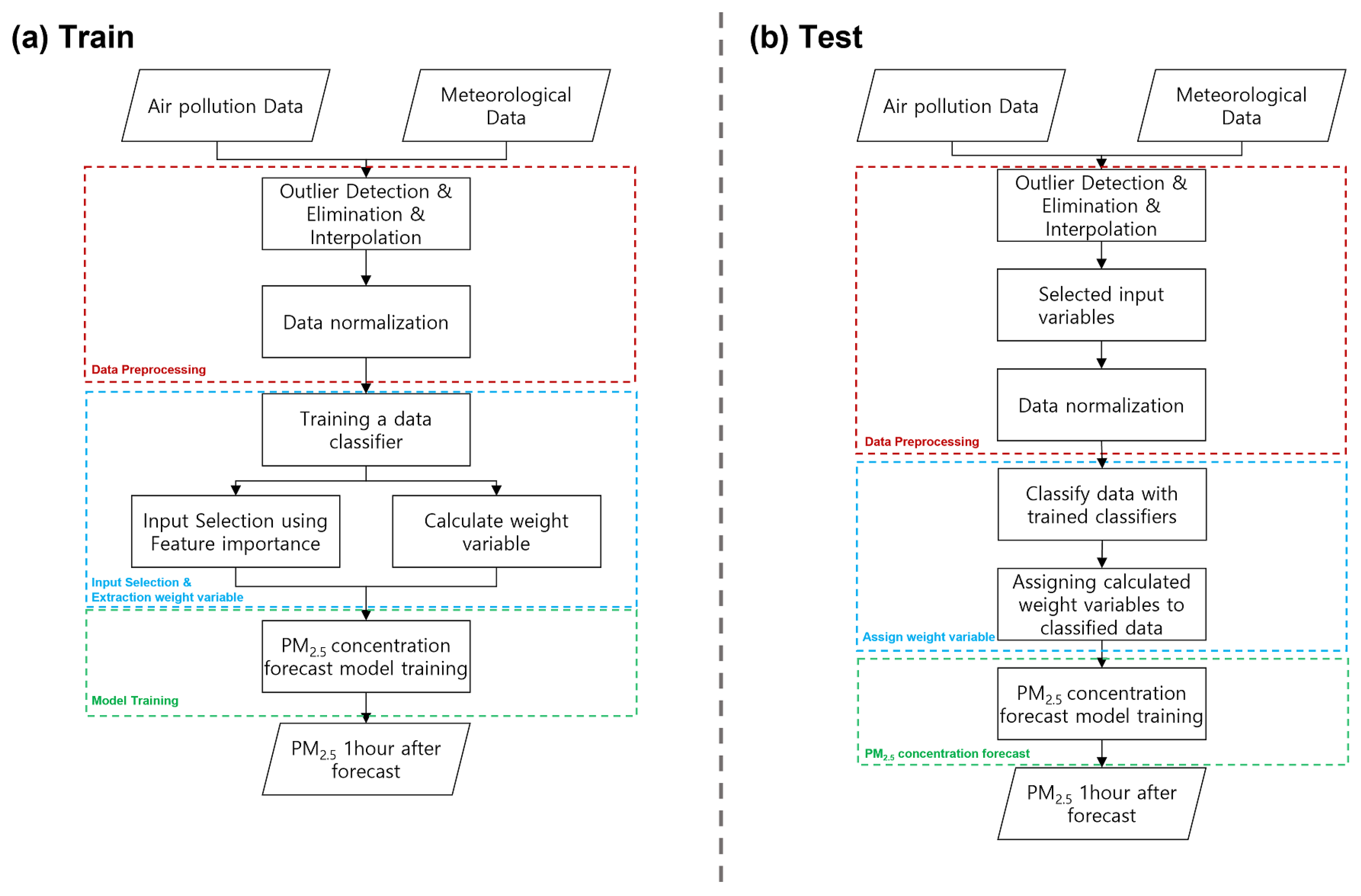
Figure 1 shows a flowchart of the PM${}_{2.5}$ concentration forecast method proposed in this study. Figure 1a shows a flowchart for training a model to forecast PM${}_{2.5}$ concentrations, and Figure 1b shows a flowchart for testing the trained models to forecast PM${}_{2.5}$ concentrations. In the preprocessing step, the outliers were removed from the air pollution and meteorological datasets. Any missing values in the data were obtained using linear interpolation. The preprocessed data were then normalized using the min–max normalization method. To select the input variables for the PM${}_{2.5}$ concentration forecast model and generate weight variables to handle the data imbalance problem, we employed a random forest model to classify the data into four grades (Good, Normal, Bad, and Worst). Classified data were assigned weight variables, and a Bi-LSTM model was applied to the selected input variables to train the PM${}_{2.5}$ concentration forecast model.

2.1. Study Sites and Data

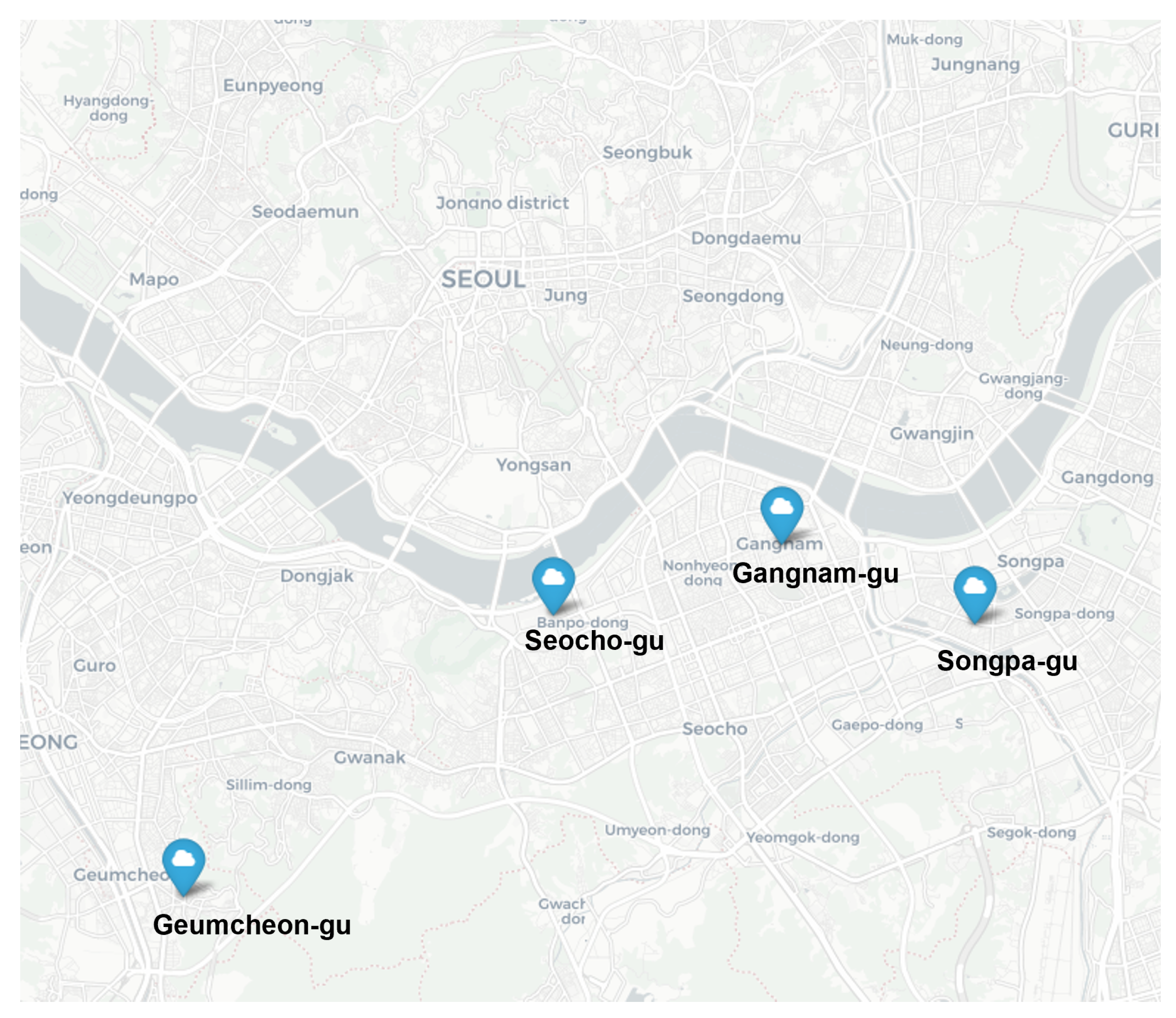
In South Korea, air quality monitoring stations operated by the South Korean Ministry of Environment are used to measure the average air quality concentrations in urban areas. This helps understand the air pollution status, changes, and whether air quality standards are met. In this study, we used air quality monitoring stations operated by the Korean Ministry of Environment in Seoul’s Gangnam-gu, Geumcheon-gu, Seocho-gu, and Songpa-gu neighbourhoods. The station locations are shown in Figure 2, and information on their locations are listed in

Table 1. Information on the air quality monitoring stations.

Monitoring Station	Address	Latitude	Longitude
Gangnam-gu	426, Hakdong-ro	37.5176${}^{\circ }$	127.0475${}^{\circ }$
Geumcheon-gu	20 Geumha-ro 21-gil	37.4524${}^{\circ }$	126.9083${}^{\circ }$
Seocho-gu	16 Sinbanpo-ro 15-gil	37.5045${}^{\circ }$	126.9944${}^{\circ }$
Songpa-gu	236, Baekjegobun-ro	37.5028${}^{\circ }$	127.0925${}^{\circ }$

. The stations represent the air quality in the southern region of Seoul, specifically in the area located south of the Han River.

Table 2. Sampling time and units for data variables.

Data	Variable	Unit	Sampling Time
Meteorological data	Precipitation type	code	1 h
	Relative humidity	%	1 h
	Precipitation	mm	1 h
	Sky condition	code	1 h
	Temperature	°C	1 h
	Thunderbolt	code	1 h
	Wind direction	degree	1 h
	Wind speed	m/s	1 h
Air pollution data	PM${}_{10}$	$\mathsf{\mu }$g/m${}^3$	1 h
	PM${}_{2.5}$	$\mathsf{\mu }$g/m${}^3$	1 h
	O${}_3$	ppm	1 h
	SO${}_2$	ppm	1 h
	NO${}_2$	ppm	1 h
	CO	ppm	1 h

presents the sampling times and data units used in this study. Meteorological data were provided by the Republic of Korea Meteorological Administration [35], which provides eight variables (precipitation type, relative humidity, precipitation, sky condition, temperature, thunderbolt, wind direction, and wind speed) at 1 h intervals for each region. Three of the eight variables included in the dataset (precipitation type, sky condition, and thunderbolts) are graded on a scale. Precipitation type is indexed from 0 to 3, where 0 indicates clear skies, 1 represents rain, 2 represents sleet, and 3 represents snow. The sky condition is indicated by an index ranging from 1 to 4, which represents sky visibility index. A value closer to 1 indicates clearer skies, whereas a value closer to 4 indicates flowing weather conditions. Thunderbolt is represented by a Boolean, which indicates the presence or absence of thunder. Air pollution data were provided by Airkorea [36], a service of the Korean Ministry of Environment, which measures the concentration of six pollutants (PM${}_{2.5}$, PM${}_{10}$, sulphur dioxide (SO${}_2$), ozone (O${}_3$), nitrogen dioxide (NO${}_2$), and carbon monoxide (CO)) at monitoring stations every hour. Air pollution data are used in both data and meteorological data, except for thunderbolts.

Table 3. Data range by monitoring station.

Type	Variable	Range
		Monitoring Station
		Gangnam-gu	Geumcheon-gu	Seocho-gu	Songpa-gu
Meteorological data	Precipitation type	0∼3	0∼3	0∼3	0∼3
	Relative humidity	10∼100	9∼100	11∼100	13∼100
	Precipitation	0∼31.8	0∼37.1	0∼48	0∼63.4
	Sky condition	1∼4	1∼4	1∼4	1∼4
	temperature	−17.3∼40.6	−17.2∼38.4	−17.4∼39.6	−16.6∼40
	Thunderbolt	0∼1	0∼1	0∼1	0∼1
	Wind direction	0∼360	0∼360	0∼360	0∼360
	Wind speed	0∼11.6	0∼7.1	0∼11.3	0∼11
Air pollution data	PM${}_{10}$	1∼926	1∼329	1∼926	1∼858
	PM${}_{2.5}$	1∼175	1∼158	1∼169	1∼140
	O${}_3$	0.001∼0.145	0.001∼0.155	0.001∼0.145	0.001∼0.114
	SO${}_2$	0.004∼0.114	0.001∼0.118	0∼0.104	0.001∼0.114
	NO${}_2$	0.1∼1.6	0.1∼1.9	0.1∼3.4	0∼2.7
	CO	0.002∼0.024	0.001∼0.028	0.001∼0.21	0.001∼0.025

presents the range of data observed at each monitoring station. Precipitation type, sky conditions, and wind direction exhibit ranges of 0–3, 1–4, and 0–360 across all stations. Relative humidity ranges from 9 to 100, while temperature and precipitation range from −17.4–40.6 and 0–63.4, respectively. Gangnam-gu exhibits the lowest maximum of precipitation values among all stations, whereas Songpa-gu has the highest. The wind speed ranges from 0 to 11.6, with Geumcheon-gu and Gangnam-gu reporting the lowest and highest values, respectively, at 7.1 and 11.6. Regarding air pollution data, PM${}_{10}$ ranges from 1 to 993, with the lowest maximum value observed in Geumcheon-gu at 329 and the highest in Seocho-gu at 993, exhibiting a significant difference of 664. PM${}_{2.5}$, ranged from 1 to 175, and the maximum value varied across stations, with the lowest reported in Songpa-gu at 140 and the highest in Gangnam-gu at 175. The range for O${}_2$ is 0.001–0.169, while the range for NO${}_2$ is 0–0.169. CO ranges from 0.1 to 3.4, and SO${}_2$ ranges from 0.001 to 0.028. Owing to the variability in the data range across monitoring stations, individual forecast models are required to provide accurate forecasts. In this study, min-max normalization was applied to the data from each monitoring station to normalize the data. The normalization equation used in this study is expressed in Equation (1), where y${}_{max}$ and y${}_{min}$ represent the maximum and minimum values of the normalization range, respectively, which were set to 1 and −1, respectively. Moreover, max(X) and min(X) represent the maximum and minimum values of the variable X, respectively.

$$X_{normalization}=y_{min}+\frac{(X-min\left(X\right))(y_{max}-y_{min})}{max\left(X\right)-min\left(X\right)}.$$

(1)

2.2. Input Selection

To achieve an accurate forecasting of PM${}_{2.5}$ concentrations, it is crucial to carefully select the influential input variables. Including unnecessary input variables in the model can increase the complexity and reduce forecasting performance. Thus, selecting appropriate input variables is essential for implementing the forecast model. In this study, the feature importance is calculated as shown in Equation (2) [37] to select the necessary input variables when classifying data labels. This is an embedded method that selects the input variables by calculating their importance when learning a model. In Equation (2), FI${}_j$ indicates the j-th feature importance and T${}_m$ indicates the m-th decision tree. I indicates the indicator function. Δp${}_m$ represents the weight difference when splitting the t-th node in the m-th decision tree. Equation (3) is used to find Δp${}_m$. In Equation (3), p${}_{left,m}$(t), p${}_{right,m}$(t), and p${}_{parent,m}$(t) represent the weight ratios of the left, right, and parent of the t-th node, respectively, of the m-th decision tree. Moreover, i${}_{left,m}$(t), i${}_{right,m}$(t), and i${}_{parent,m}$(t) represent the impurity for the left, right, and parent of the t-th node, respectively, of the m-th decision tree.

$$F{I}_j=\frac{1}{M}\sum _{m=1}^M\sum _{t=1}^{T_m}I(j_t=j)▵p_m\left(t\right),$$

(2)

$$▵p_m\left(t\right)=p_{left,m}\left(t\right)i_{left,m}\left(t\right)+p_{right,m}\left(t\right)i_{right,m}\left(t\right)-p_{parent,m}\left(t\right)i_{parent,m}\left(t\right).$$

(3)

2.3. Imbalanced Data

In South Korea, PM${}_{2.5}$ levels are managed through classification based on concentration. The concentration range for each grade is presented in

Table 4. Grade range of particulate matter concentration.

Grade	Range
Good	0 ≤ PM${}_{2.5}$ ≤ 15
Normal	16 ≤ PM${}_{2.5}$ ≤ 35
Bad	36 ≤ PM${}_{2.5}$ ≤ 75
Worst	76 ≤ PM${}_{2.5}$

, where “Good” corresponds to a concentration greater than 0 and less than 15, “Normal” corresponds to a concentration greater than 16 and less than 35, “Bad” corresponds to a concentration greater than 36 and less than 75, and “Worst” corresponds to a concentration greater than 76.

Table 5. Ratio of data grade by station.

Station	Number of Data
	Gangnam-gu	Geumcheon-gu	Seocho-gu	Songpa-gu
Good	6900 (30.2%)	6239 (26.66%)	7764 (33.08%)	8236 (34.59%)
Normal	11,324 (49.56%)	11,863 (50.7%)	11,744 (50.03%)	11,664 (48.45%)
Bad	4269 (18.68%)	4934 (21.09%)	3714 (15.82%)	3884 (16.13%)
Worst	355 (1.55%)	364 (1.56%)	250 (1.07%)	198 (0.82%)
Total	22,848 (100%)	23,400 (100%)	23,472 (100%)	24,072 (100%)

presents the number of data points and the percentage of data in each grade for each of the stations. The proportion of data classified as ‘normal’ was the highest among all stations. The proportion of low-concentration data (PM${}_{2.5}$≤ 35; Good, Normal) is consistently higher than that of high-concentration data (PM${}_{2.5}$≥ 36; Bad, Worst) across all stations. Training a model with such a proportion of data will lead to a low-concentration bias. We used the weighting method, which is cost sensitive, to solve the data imbalance problem. The weighting method assigns weights to a small number of classes to learn unbiasedly from a large amount of data. In addition, unlike the sampling method, it does not lose information about the data and is not affected by the problem of generalization ability deterioration owing to the generation of redundant data. To assign weights, we categorized it into four grades (Good, Normal, Bad, and Worst). The random forest method was used for data classification. Random forest [38] is a supervised ensemble learning method that uses multiple decision trees to select many outcomes that can be used for classification and regressions. Since this method combines multiple decision trees to make forecasts, it reduces the bias and variance of the model to solve the overfitting problem, resulting in a relatively high forecast performance. Additionally, the importance of a variable can be calculated using this model. Since the data distribution and range of each station differs, the models were trained separately for each station and for Bayesian optimization [39].

Table 6. Parameters of the random forest by station.

Monitoring Station	Optimum Value
	Number of Trees	Learning Rate	Criterion
Gangnam-gu	52	0.9853	Gini diversity index
Geumcheon-gu	10	0.5267	Gini diversity index
Seocho-gu	16	0.7445	Gini diversity index
Songpa-gu	17	0.7364	Gini diversity index

lists the parameters of the model used in each station to train the random forest.

To assign weight variables to the data classified into four grades (Good: 1, Normal: 2, Bad: 3, Worst: 4), the probability of each class was calculated by computing the proportion of data in each class. We then used Equation (4), where c denotes a class, Nc denotes the number of data points in the c-th class, and k represents the total number of data classes. Equation (4) is simple to calculate and is an intuitive method. The resulting value of Equation (4) is highly weighted towards prime number data, which can lead to better learning. By applying Equation (4) we obtained the weight variable value (cw${}_c$) for the c-th class.

$$c{w}_c=\frac{\frac{1}{N_c}}{{\sum }_{c=1}^k\frac{1}{N_c}}.$$

(4)

2.4. Bidirectional Long Short-Term Memory

To address the challenge of long-term dependence in traditional recurrent neural networks (RNNs), which arises owing to the vanishing or exploding gradient problem when processing long sequence data, Hochreiter and Schmidhuber proposed LSTM [40]. LSTM consists of a forget gate (f${}_t$), input gate (i${}_t$), update gate (g${}_t$), output gate (o${}_t$) and a cell state (c${}_t$). Equations (5)–(9) compute each gate and cell state of the LSTM at time t. In each equations, $\sigma$ represents a sigmoid function, and tanh is the hyperbolic tangent function. x${}_t$ represents the input vector at time t, and h${}_{t-1}$ represents the hidden layer output at time $t-1$. W and b denote the weight and bias of the equations, respectively. Equation (5) expresses the forget gate operation, which determines which information to retain from the previous time point.

$$f_t=\sigma (W_f[x_t,h_{t-1}]+b_f),$$

(5)

The input gate is calculated using Equation (6) and is responsible for determining which of the new information should be stored in the cell state.

$$i_t=\sigma (W_i[x_t,h_{t-1}]+b_i),$$

(6)

The update gate is a function that determines the amount of information to store in the current cell state, calculated using Equation (7).

$$g_t=tanh(W_i[x_t,h_{t-1}]+b_c),$$

(7)

The output gate is calculated using Equation (8) and is the gate that determines what information to output.

$$o_t=\sigma (W_o[x_t,h_{t-1}]+b_o),$$

(8)

The cell state is calculated by multiplying the cell state of the previous time by a value of the forget gate, as shown in Equation (9), and then adding the product of the outputs of the input gate and value of the update gate to add new information. The cell state contains information from the previous time to the current time.

$$c_t=f_t\odot c_{t-1}+i_t\odot g_t,$$

(9)

Calculate h${}_t$ at time t using the calculated cell state and output gate. Equation (10) is used to calculate h${}_t$.

$$h_t=o_t\odot tahn\left(c_t\right).$$

(10)

LSTM was proposed to address the long-term dependence encountered by traditional RNNs when processing long sequence data, they are still constrained by their unidirectional processing. To overcome this limitation, Bi-LSTM was introduced [41]. Bi-LSTM performs operations on the forward LSTM and on the backward LSTM. Figure 3 shows backward LSTM in Bi-LSTM.

In Figure 3, the backward layer consists of the same four gates (forget gate, input gate, update gate, and output gate) and cell state as the forward layer. Unlike the gate operation of the forward layer, the backward layer uses the output value of the hiding layer at t + 1 as the input of each gate. The output values of the forward and backward layers are then combined to determine the output value of the hidden layer. Since the Bi-LSTM can consider both the forward and backward directions of the data, it can better reflect the information generated at both ends. It can also utilize a large amount of information because it uses the input data once again.

The Bi-LSTM is a type of neural network where the performance varies depending on the number of nodes in the hidden layer. To select the appropriate number of hidden nodes, we performed forecasts by increasing the number of nodes in the hidden layer from 16 (2${}^4$) to 128 (2${}^7$) in a doubling fashion [42,43]. The optimal number of hidden nodes was determined as the one that resulted in the lowest root mean square error (RMSE). Each model was optimized using the Adam (adaptive moment estimation) method [44].

Table 7. RMSE results based on the number of hidden layer nodes for stations of Gangnam-gu and Geumcheon-gu.

Number of Nodes in the 1st Hidden Layer	Number of Nodes in the 2nd Hidden Layer
	Gangnam-gu				Geumcheon-gu
	16	32	64	128	16	32	64	128
16	6.027	5.971	6.006	5.991	3.606	3.611	3.602	3.600
32	6.028	6.015	6.010	6.024	3.577	3.626	3.622	3.647
64	5.969	5.926	6.000	6.003	3.629	3.592	3.569	3.598
128	5.998	6.017	5.958	5.970	3.590	3.582	3.625	3.605

and

Table 8. RMSE results based on the number of hidden layer nodes for stations of Seocho-gu and Songpa-gu.

Number of Nodes in the 1st Hidden Layer	Number of Nodes in the 2nd Hidden Layer
	Seocho-gu				Songpa-gu
	16	32	64	128	16	32	64	128
16	5.654	5.776	5.658	5.764	5.345	5.419	5.321	5.337
32	5.730	5.642	5.723	5.727	5.326	5.359	5.389	5.354
64	5.667	5.683	5.646	5.719	5.314	5.383	5.406	5.361
128	5.717	5.736	5.684	5.733	5.419	5.396	5.395	5.353

shows the RMSE calculation results by the number of covert layer nodes for each station. Where RMSE represents the RMSE of the training data, and bold indicates the lowest RMSE per station.

Table 9. Training options of the forecast model for selecting the number of hidden nodes.

Training Option	Training Option Value
minibatchsize	32
maxEpoch	1000
Initial Learning Rate	0.001
EarlyStopping	15

shows the training options for the model used to select the number of hidden layer nodes.

Table 10. Structure of the hidden layer for each monitoring station.

Station	Attribution	Layer
		1st	2nd	3rd	4th
Gangnam-gu	Layer type	Bi-LSTM	Bi-LSTM	FC	FC
	Number of nodes	64	32	24	1
Geumcheon-gu	Layer type	Bi-LSTM	Bi-LSTM	FC	FC
	Number of nodes	64	64	24	1
Seocho-gu	Layer type	Bi-LSTM	Bi-LSTM	FC	FC
	Number of nodes	32	32	24	1
Songpa-gu	Layer type	Bi-LSTM	Bi-LSTM	FC	FC
	Number of nodes	64	16	24	1

presents the number of nodes for each hidden layer, where FC denotes a fully connected layer.

3. Experiments and Results

Air pollution data and meteorological data were used to forecast the PM${}_{2.5}$ concentration. Data from four years (2015–2018) were used in the forecasting, and the training data were from three years (2015–2017), and the test data was from 2018. To compare the performance of the proposed model, we performed experiments for two cases. In case study 1, we selected input variables to reduce the complexity of the model and increase its comprehensibility and added weighting variables to solve the data imbalance problem and compared the results of forecasting the model without doing so. Case study 2 compares the performances of three deep learning models (LSTM, Bi-LSTM, and GRU) and conventional machine learning models (MLP, SVM, decision tree, random forest) by the station to compare the performances of the forecast models in the proposed method. In both experiments (case study 1 and 2), in order to consider the past time points and that from the current time point (t) to 23 h before the past time, point (t $- 23$) was used as the input to forecast one hour (t $+ 1$) later.

3.1. Performance Index

To numerically compare the experimental results of the case study, we used three performance indices used in regression: RMSE, mean absolute error (MAE), relative root mean square error (RRMSE), and R${}^2$. The RMSE was obtained by averaging the squares of the error difference between the forecast and actual values and taking the square root of the result. The MAE was calculated as the mean of the absolute errors. The RRMSE is the relative value of the RMSE between the forecasted and actual values divided by the average of the actual values. The lower the values of RMSE, MAE, and RRMSE, the better the forecasting performance. R${}^2$ is an index that evaluates the extent to which the forecast describes its true value. R${}^2$ has a value between 0 and 1. The closer it is to 1, the better the model describes the data. Equations (11)–(14) are used to determine RMSE, MAE, RRMSE, and R${}^2$. In each of these formulas, ${\widehat{y}}_i$ refers to the i-th forecasted value, and y${}_i$ refers to the i-th observed value, where $\overline{y}$ denotes the mean of the observed values.

$$RMSE=\sqrt{\frac{1}{n}\sum _{i=1}^n{(y_i-{\widehat{y}}_i)}^2}.$$

(11)

$$MAE=\frac{1}{n}\sum _{i=1}^n\left|(y_i-{\widehat{y}}_i)\right|.$$

(12)

$$RRMSE=\frac{\sqrt{\frac{1}{n}{\sum }_{i=1}^n{(y_i-{\widehat{y}}_i)}^2}}{\overline{y}}.$$

(13)

$$R^2=r^2=1-\frac{{\sum }_{i=1}^n{(y_i-{\widehat{y}}_i)}^2}{{\sum }_{i=1}^n{(y_i-{\overline{y}}_i)}^2}.$$

(14)

3.2. Case Study 1: Comparing the Conventional Method with the Proposed Method

Case study 1 compares the proposed method with the conventional method. The conventional method forecasts using all the variables in the data. The proposed method uses a random forest to select the input variables and a weight variable to solve the unbalanced data and uses Bi-LSTM to forecast the PM${}_{2.5}$ concentration. The results of calculating the feature importance using a random forest to select the input variables are shown in

Table 11. Feature importance value by station.

Data	Variable	Monitoring Station
		Gangnam-gu	Geumcheon-gu	Seocho-gu	Songpa-gu
Meteorological data	Precipitation type	0	0	0	0
	Relative humidity	0	0.0001	0	0
	Precipitation	0	0	0	0
	Sky condition	0	0	0	0
	temperature	0.0001	0.0001	0.0001	0
	Wind direction	0	0.0001	0	0
	Wind speed	0	0	0	0
Air pollution data	PM${}_{10}$	0.0006	0.0001	0.0003	0.0005
	PM${}_{2.5}$	0.0132	0.0179	0.0132	0.0133
	O${}_3$	0.0001	0.0001	0.0001	0.0001
	SO${}_2$	0.0001	0.0001	0.0001	0.0003
	NO${}_2$	0.0002	0.0001	0.0002	0
	CO	0	0.0001	0	0

. In Table 11, PM${}_{2.5}$ has the highest value for all monitoring stations. PM${}_{10}$ is the second highest at all stations except Geumcheon-gu. Among the meteorological variables, the temperature had the highest value at all stations except Songpa-gu. Among the values calculated in Table 11, non-zero and weight variables were used as input variables for the forecasting model.

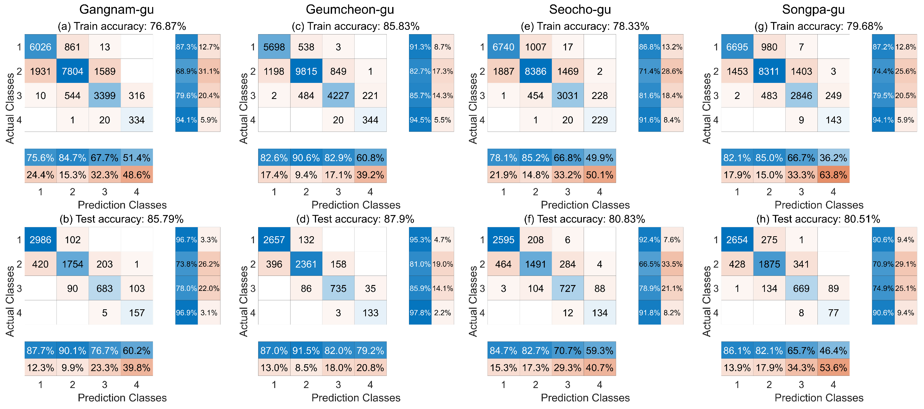
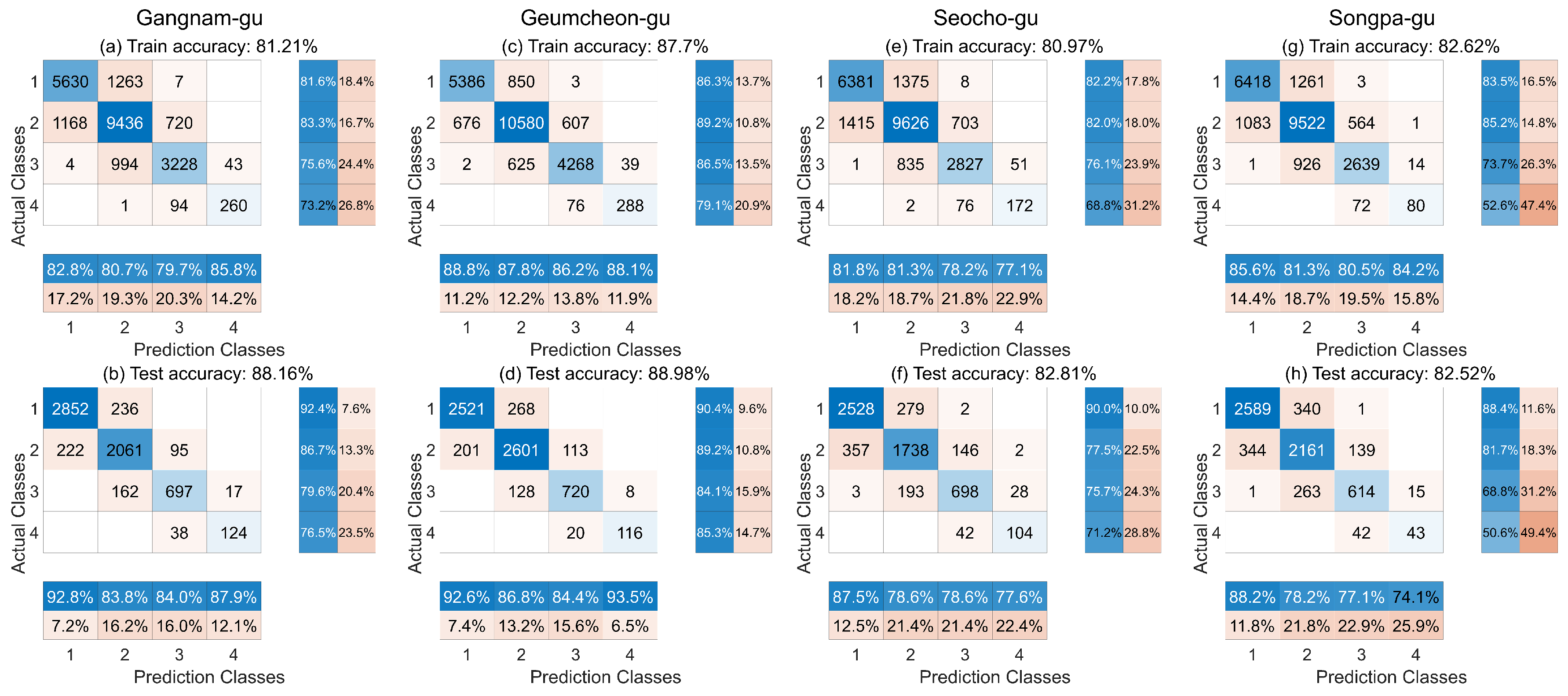
In addition, to assign weighting variables, the data must be classified by thePM${}_{2.5}$ class. Therefore, this paper performs the classification using a random forest. The input variables are the same as those of the forecasting model selected earlier. Since each monitoring station has a different data range and distribution, they were trained separately, and the input variables at time t were used to classify the PM${}_{2.5}$ class at time t$+1$. To compare the classification accuracy according to the selection of input variables, we conducted experiments before and after the selection of input variables. Figure 4 and Figure 5 show the confusion matrix before and after the selection, respectively. In each figure, (a) and (b) show the confusion matrices for Gangnam-gu, (c) and (d) for Geumcheon-gu, (e) and (f) for Seocho-gu, and (g) and (h) for Songpa-gu. Using input selection for data classification improved the training and test data classification accuracy. The most considerable improvement was observed for Gangnam-gu, where the accuracy increased by 4.34%p in the training data and 2.37%p in the test data.

The results of calculating the weighting variables are shown in

Table 12. Values of the weighing variables by station.

Grade	Monitoring Station
	Gangnam-gu	Geumcheon-gu	Seocho-gu	Songpa-gu
Good	0.0441	0.0502	0.0287	0.0184
Normal	0.0269	0.0264	0.0190	0.0126
Bad	0.0713	0.0634	0.0601	0.0395
Worst	0.8577	0.8600	0.8922	0.9295
Total	1	1	1	1

. In Table 12, ’Worst’ has the smallest data percentage and the highest weighting variable.

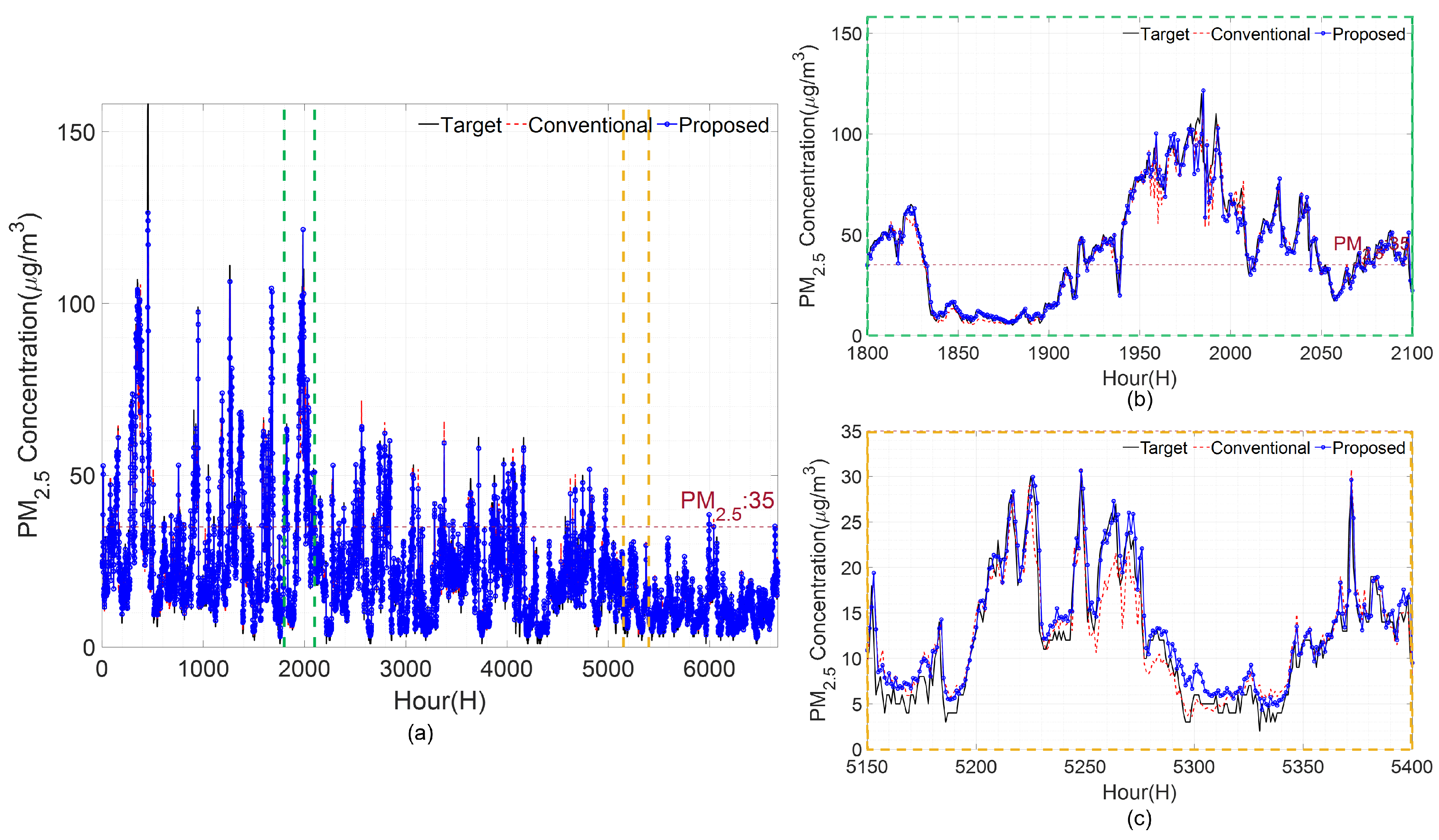
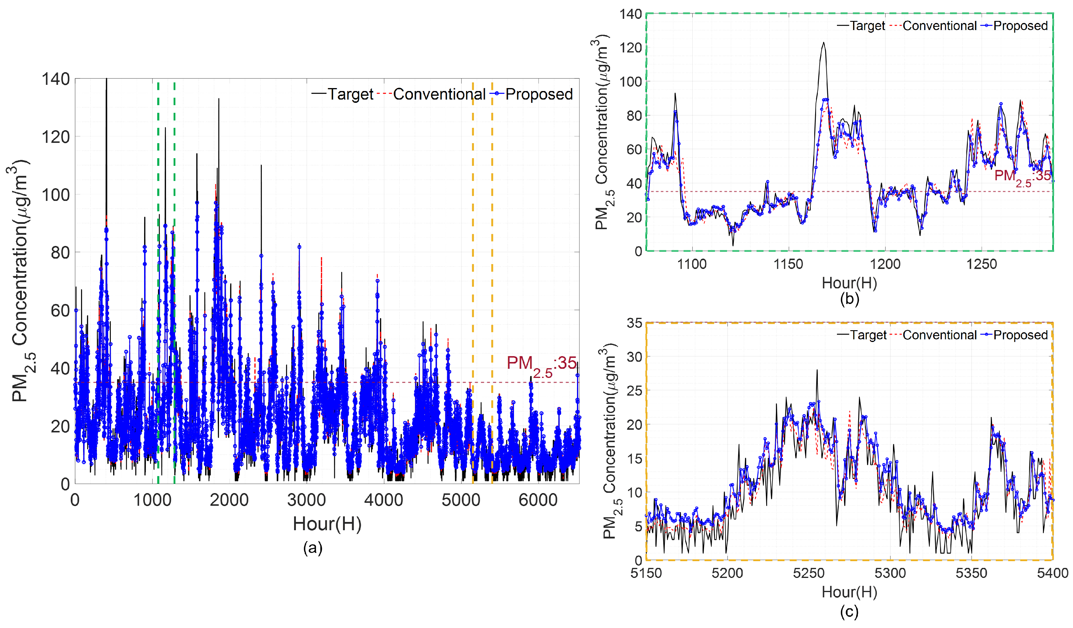
Figure 6, Figure 7, Figure 8 and Figure 9 show the forecast results of each station using the conventional and proposed methods. In the figures shown in Figure 6, Figure 7, Figure 8 and Figure 9, (a) shows the test period; (b) shows the period between the two green dashed lines, which is a section of active high-concentration; while (c) shows the period between the two yellow dashed lines, which corresponds to a low-concentration section. The x-axis in the figure represents time, and the y-axis represents the concentration. The black solid line represents the actual PM${}_{2.5}$ concentration measured at each monitoring station, while the red dashed line represents the forecasted value using the conventional method. The blue circled line represent the forecasted values obtained using the proposed method. The magenta dotted line indicates the threshold value of the PM${}_{2.5}$ concentration at 35, which is the standard for high concentration. The proposed and conventional methods are under forecasting when forecasting the PM${}_{2.5}$ concentration in Gangnam-gu. Between 445 and 450 h, the target value continues to increase, and the forecast value of the conventional method decreases. However, the proposed method exhibits a lower error in forecasting by increasingly following the target value. In the low-concentration period (Figure 6c), the forecast result of the conventional method is under forecast, and it is evident that the forecast performance is lower than that of the proposed method in the 5250–5300 h. In the high-concentration section of Geumcheon-gu (Figure 7b), which spans from 1950 to 1980 h, the conventional method shows a sharp decrease in forecasted values, while the proposed method forecasts the target PM${}_{2.5}$ concentrations. In Figure 7c, which shows the forecast result of the low-concentration section, the proposed method forecasts better than the conventional method. In the high-concentration section of Seocho-gu, the conventional and proposed methods are primarily under forecasting. The proposed method has a better forecast performance from 330 to 380 h, where the concentration is above 75 and changes rapidly. For the low-concentration section, the conventional method over forecasts compared with the proposed method and has a lower forecast performance than the proposed method. For the high-concentration section of Songpa-gu, between 1090 and 1095 h, the conventional method does not forecast more than 60, while the proposed method forecasts up to 80, exhibiting a lower error. However, from 1165 to 1170 h, where the concentration is above 100, both methods have errors due to under forecasting.

In Figure 6, Figure 7, Figure 8 and Figure 9b, the high-concentration range of each station, it can be seen that the conventional method under forecasts the proposed method because it is trained with a bias towards low-concentration, which is the major class data.

Table 13. RMSE for the forecast results of the conventional method and the proposed method.

	Test Period		High-Concentration Section		Low-Concentration Section
Station	Conventional Method	Proposed Method	Conventional Method	Proposed Method	Conventional Method	Proposed Method
Gangnam-gu	4.7384	4.4122	8.3142	7.7802	3.6736	3.4035
Geumchoen-gu	3.9179	3.8180	7.3199	7.1371	2.9432	2.8867
Seocho-gu	6.5666	6.2922	11.0503	10.9497	5.1178	4.7378
Songpa-gu	5.8446	5.7073	10.8168	10.4297	4.4210	4.3750
Average	5.2669	5.0574	9.3753	9.0724	4.0389	3.8458

,

Table 14. MAE for the forecast results of the conventional method and the proposed method.

	Test Period		High-Concentration Section		Low-Concentration Section
Station	Conventional Method	Proposed Method	Conventional Method	Proposed Method	Conventional Method	Proposed Method
Gangnam-gu	3.4142	3.0561	6.4705	5.9106	2.8313	2.5116
Geumchoen-gu	2.5575	2.4637	5.1476	4.9232	2.1051	2.0341
Seocho-gu	4.6788	4.3381	8.1944	8.1732	3.9321	3.5235
Songpa-gu	4.0299	3.9606	7.8609	7.4588	3.3556	3.3449
Average	3.6701	3.4546	6.9184	6.6165	3.0560	2.8535

,

Table 15. RRMSE for the forecast results of the conventional method and the proposed method.

	Test Period		High-Concentration Section		Low-Concentration Section
Station	Conventional Method	Proposed Method	Conventional Method	Proposed Method	Conventional Method	Proposed Method
Gangnam-gu	0.2203	0.2052	0.1486	0.1390	0.2460	0.2279
Geumchoen-gu	0.1777	0.1732	0.1349	0.1315	0.1792	0.1758
Seocho-gu	0.3053	0.2926	0.2019	0.2000	0.3543	0.3280
Songpa-gu	0.2775	0.2710	0.2118	0.2043	0.2801	0.2772
Average	0.2452	0.2355	0.1743	0.1687	0.2648	0.2522

and

Table 16. R${}^2$ for the forecast results of the conventional method and the proposed method.

	Test Period		High-Concentration Section		Low-Concentration Section
Station	Conventional Method	Proposed Method	Conventional Method	Proposed Method	Conventional Method	Proposed Method
Gangnam-gu	0.9366	0.9451	0.9928	0.9937	0.8463	0.8680
Geumchoen-gu	0.9476	0.9502	0.9940	0.9943	0.8828	0.8888
Seocho-gu	0.8861	0.8955	0.9855	0.9858	0.7233	0.7631
Songpa-gu	0.8748	0.8806	0.9850	0.9861	0.7760	0.7806
Average	0.9113	0.9179	0.9893	0.9900	0.8071	0.8251

list the RMSE, MAE, RRMSE and R${}^2$ values of the conventional and proposed methods, respectively. The values in each table are the averages of the results of 10 iteration experiments. As listed in Table 10, the proposed method has an average RMSE of 0.2095 (3.98%p), which is lower than that of the conventional method. Specifically, in the high-concentration section, the proposed method is 0.3011 (3.21%p) lower than the conventional method. Notably, the Gangnam-gu forecast model shows the most significant difference, with the proposed method differing from the conventional method by 0.3262 (6.88%p) for the overall RMSE and 0.534 (6.42%p) for the RMSE of the high-concentration section. Furthermore, even in the low-concentration section, the proposed method shows an average RMSE of 0.1931 (4.78%p), which is lower than that of the conventional method, with the smallest difference of 0.38 (7.43%p) observed for Songpa-gu. Additionally, the performance improvement of the proposed method is more significant in the high concentration range for Geumcheon-gu and Seocho-gu stations. Table 14 indicates that the proposed method has, on average, a 5.87% lower MAE than the conventional method. In the high-concentration section, the proposed method outperforms the conventional method by 4.36% for all stations. Moreover, the proposed method exhibits a 6.63% lower MAE than the conventional method in the low-concentration section. The largest differences in MAE between the proposed and conventional methods are observed for the stations in Gangnam-gu, with reductions of 10.49, 8.65, and 11.29%, respectively, for the entire test period, high-concentration, and low-concentration sections, respectively. Among the high-concentration sections, the station in Songpa-gu shows the largest difference of 0.0011 (0.11%p). Table 15 shows that the proposed method is, on average, 0.0097 (3.96%p) lower than the conventional method. In the high-concentration range, the proposed method is lower on average by 0.0056 (3.21%p), with the largest difference (0.0096, 6.46%p) in Gangnam-gu. In the low-concentration range, the proposed method is also lower than the conventional method by 0.013 (4.76%p), with the most significant difference (0.0263, 7.42%p) in Seocho-gu. Table 16 shows that the R${}^2$ value of the proposed method is 0.0066 (0.72%p) higher than the conventional method. In the high-concentration range, the proposed method is higher by 0.0007 (0.07%p). Especially in the high-concentration range, Songpa-gu shows the most significant difference of 0.0011 (0.11%p). In the low-concentration range, the proposed method is also higher than the conventional method by 0.018 (2.23%p). Especially in Seocho-gu, the proposed method is higher than the conventional method by 0.0094 (1.06%p) and 0.0398 (5.50%p) in the test period and low-concentration range.

3.3. Case Study 2: Comparing the Deep Learning Model and Conventional Machine Learning

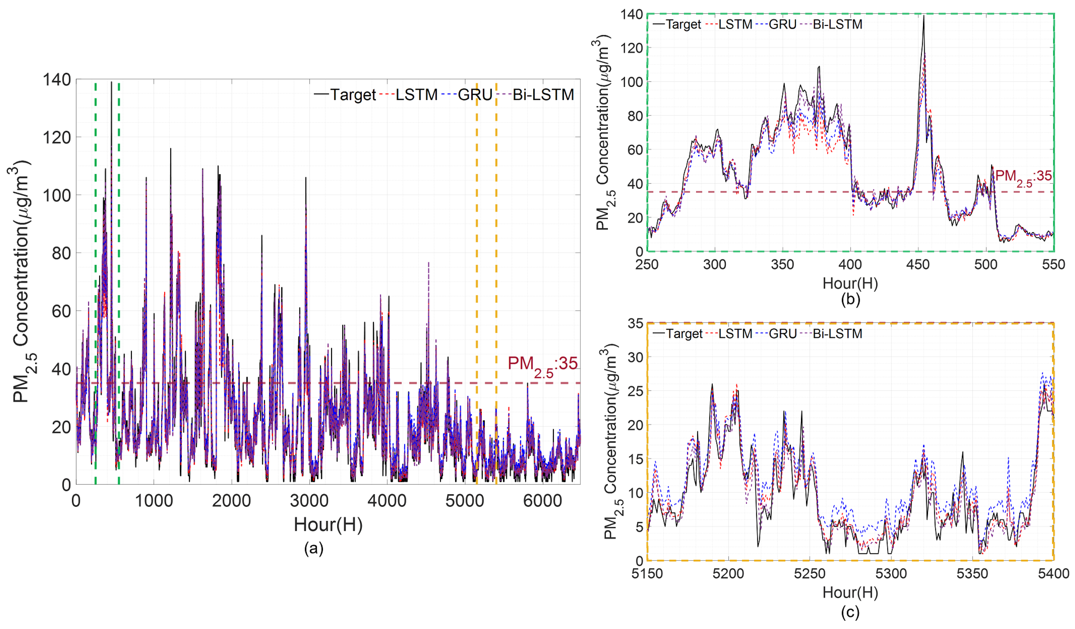
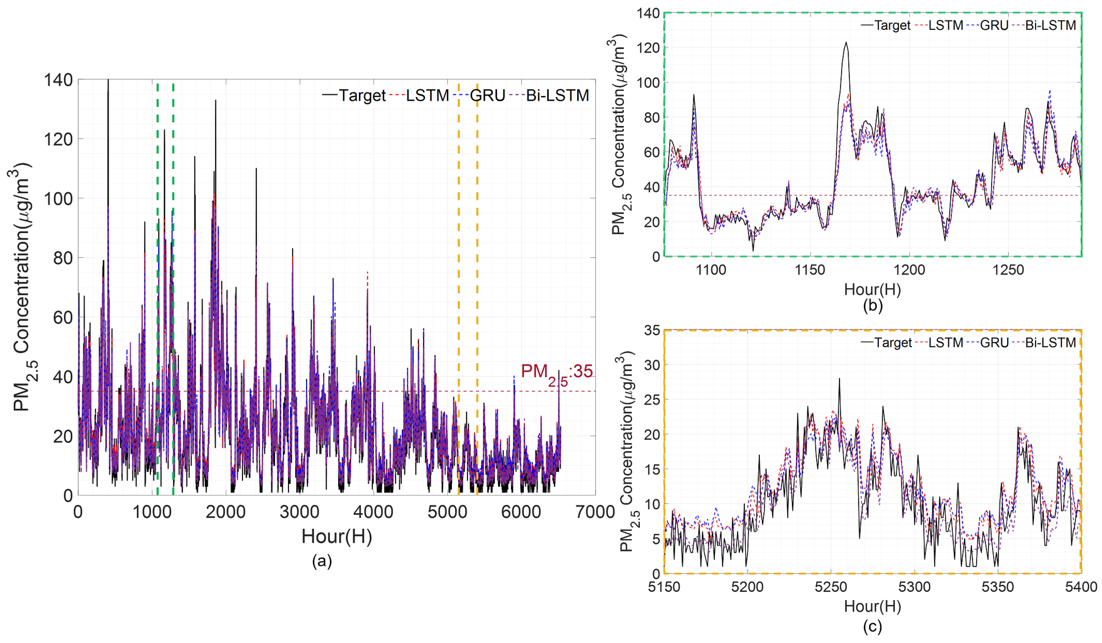
In case study 2, we evaluate the forecasting accuracy of PM${}_{2.5}$ concentrations using deep learning models (LSTM, GRU, and Bi-LSTM) with superior forecasting performance and conventional used machine learning models (MLP, SVM, DT, and RF). The input variables of the models are those proposed in case study 1. The forecast results of the LSTM, GRU, and Bi-LSTM models for each station are illustrated in Figure 10, Figure 11, Figure 12 and Figure 13. The x-axis represents time, and the y-axis represents the PM${}_{2.5}$ concentration. The black line represents the actual values of each station, while the red and blue dashed lines indicate the forecasting results of the LSTM and GRU models. The forecast result of Bi-LSTM is indicated by the purple dashed line. The magenta-coloured dotted line represents the point where the PM${}_{2.5}$ concentration value is 35. In each figure, (a) represents test periods; (b) represents the period between the two green dashed lines, which are sections of high-concentration; while (c) shows the period between the two yellow dashed lines, which is the low-concentration section.

Regarding comparing forecast performance among different models in case study 2, it can be observed that all models underestimate the actual PM${}_{2.5}$ concentration in the high-concentration section of Gangnam-gu shown in Figure 10b. However, the Bi-LSTM model provides the best forecasting performance among the areas with a concentration above 75, particularly between 350 and 390 h. In the low-concentration section, all models over forecast. For the high-concentration section of Geumcheon-gu, the Bi-LSTM model performs better than the other two models during 1940–2010 h, where the concentration changes rapidly. On average, in the low-concentration section, the Bi-LSTM over forecasted, while LSTM and GRU under forecasted. The Bi-LSTM exhibits better forecasting performance in the normal range of 15 and above and 35 and below. Within the PM${}_{2.5}$ concentrations between 0 and 15, LSTM exhibits the most accurate forecasting performance.

In the high-concentration section of Seocho-gu, all models under forecast on average, and Bi-LSTM outperforms LSTM and GRU in the range of 330–400 h. All models over forecast in the low-concentration section, and the GRU exhibits the best performance in the range of 0–10, followed by Bi-LSTM. For Songpa-gu, GRU exhibits the best forecasting performance in the high-concentration section of 1080–1095 h, and LSTM exhibits the best forecast performance in the increasing section of 1240–1285 h, followed by Bi-LSTM with the second best forecasting performance. In the low-concentration section, LSTM and GRU over forecast on average, while Bi-LSTM under forecasts. Therefore, it exhibits the best overall forecasting performance in this section.

Table 17. RMSE and MAE values for the deep learning models.

	RMSE			MAE
Station	LSTM	GRU	Bi-LSTM	LSTM	GRU	Bi-LSTM
Gangnam-gu	4.7690	4.7380	4.4122	3.1017	3.2853	3.0561
Geumchoen-gu	3.8340	3.9400	3.8180	2.4833	2.6173	2.4894
Seocho-gu	6.3340	6.4560	6.2992	4.3589	4.4671	4.3381
Songpa-gu	5.8930	5.7340	5.7073	4.0181	3.9954	3.9606
Average	5.2075	5.2170	5.0591	3.4905	3.5913	3.4610

and

Table 18. RRMSE and R${}^2$ values for the deep learning models.

	RRMSE			R${}^2$
Station	LSTM	GRU	Bi-LSTM	LSTM	GRU	Bi-LSTM
Gangnam-gu	0.2218	0.2203	0.2052	0.9341	0.9366	0.9451
Geumchoen-gu	0.1739	0.1787	0.1732	0.9497	0.9469	0.9502
Seocho-gu	0.2945	0.3002	0.2926	0.8940	0.8899	0.8955
Songpa-gu	0.2798	0.2722	0.2710	0.8808	0.8794	0.8806
Average	0.2425	0.2429	0.2355	0.9146	0.9132	0.9179

list the performance indices for the PM${}_{2.5}$ concentration forecast results using the deep learning model. The numbers in Table 17 and Table 18 are the averages of the results from 10 replicates. In the case of RMSE, MAE, and RRMSE, Bi-LSTM performs better at all stations except for Geumcheon-gu. Comparing the average RMSE, Bi-LSTM outperforms LSTM and GRU by 0.1405 (2.6977%p) and 0.15 (2.8748%p), respectively. Comparing the average MAE of the models, the performance of Bi-LSTM is higher than LTSM and GRU by 0.0295 (0.844%p) and 0.1302 (3.6264%p), respectively. When using Bi-LSTM, we can see that the RRMSE is lower than LSTM and GRU by 0.0070 (2.8866%p) and 0.0074 (3.0266p%), respectively. For R${}^2$, the LSTM performance is best for the Geumcheon-gu and Songpa-gu stations, whereas the Bi-LSTM performance is best for the Gangnam-gu and Seocho-gu stations. With respect to the average R${}^2$, Bi-LSTM outperforms LSTM and GRU by 0.0029 (0.3196%p) and 0.0044 (0.4759%p), respectively.

Table 19. RMSE and MAE values for the machine learning models.

	RMSE				MAE
Station	MLP	SVM	DT	RF	MLP	SVM	DT	RF
Gangnam-gu	6.3755	6.6377	7.1953	6.0420	4.5595	4.3955	5.0105	4.0118
Geumchoen-gu	6.1839	5.7206	5.4665	4.5156	4.3120	3.3895	3.7392	3.0054
Seocho-gu	9.0127	9.3729	8.3952	7.9718	6.2222	6.2260	6.0515	5.4270
Songpa-gu	6.1787	7.2686	8.2504	6.9803	4.3435	4.8768	5.7261	4.7145
Average	6.9377	7.2686	7.3269	6.3775	4.9598	4.7219	5.1318	4.3009

and

Table 20. RRMSE and R${}^2$ values for the machine learning models.

	RRMSE				R${}^2$
Station	MLP	SVM	DT	RF	MLP	SVM	DT	RF
Gangnam-gu	0.2962	0.3084	0.3343	0.2807	0.8847	0.8751	0.8532	0.8965
Geumchoen-gu	0.2805	0.2595	0.2480	0.2048	0.8691	0.8879	0.8976	0.9301
Seocho-gu	0.4260	0.4431	0.3968	0.3768	0.7785	0.7604	0.8080	0.8270
Songpa-gu	0.2899	0.3445	0.3871	0.3275	0.8688	0.8147	0.7660	0.8325
Average	0.3232	0.3389	0.3415	0.2975	0.8503	0.8312	0.8312	0.8715

show the performance index values of conventional machine learning. Among the machine learning methods, the performance index shows the best performance when forecasting is performed using RF. Compared to Bi-LSTM, the best performer in deep learning, Bi-LSTM was better than RF by RMSE: 26.96%, MAE: 32.56%, R${}_2$: 5.02%, and RRMSE: 20.83%. To summarize case study 2, Bi-LSTM has the best performance regarding RMSE, MAE, RRMSE, and R${}^2$ compared to other deep learning and machine learning methods because it considers bi-directionality to make a forecast.

3.4. Discussion

This study aims to forecast the concentration after 1 h of PM${}_{2.5}$ that can harm the human body. The proposed method is conducted in two steps; (1) selection of appropriate input variables and weight assignment using random forest, and (2) forecasting of PM${}_{2.5}$ using Bi-LSTM. Appropriate input variables for forecasting were selected by calculating the importance of each variable using RF. However, the data usually consists of imbalanced data where the categories are not proportioned. Imbalanced data can lead to bias problems and degrade predictive performance. To improve this problem, a weight variable was added according to the grade classified through RF and used as an input variable for the forecast. Finally, the PM${}_{2.5}$ concentration was forecasted by applying Bi-LSTM to the input and weight variables selected through RF. To validate the proposed method, two case studies were applied to monitoring stations in South Korea. Case study 1 (Section 3.2) compares the prediction performance according to the selection of the input variables. Case study 2 (Section 3.3) compares the forecast performance between the deep learning and conventional machine learning methods. Experimental results confirm that the proposed method is improved compared to conventional methods, such as LSTM, GRU, MLP, SVM, DT, and RF. In particular, it is shown that the prediction can be effectively performed even if there is a data imbalance problem by assigning weights using RF. In future work, we will discuss various multi-step forward forecasting strategies such as recursive, direct, and multi-input multi-output to perform long-term forecasting.

4. Conclusions

As the incidence of disease caused by PM${}_{2.5}$ exposure increases, it is essential to forecast PM${}_{2.5}$ concentrations to prevent PM${}_{2.5}$ exposure. In this study, we proposed a method for forecasting PM${}_{2.5}$ after 1 h from PM${}_{2.5}$ data with imbalanced data. Appropriate input variables were selected through RF and then used to add weight variables to improve the prediction performance. Consequently, using RF reduces model complexity and improves the forecasting performance. Then, PM${}_{2.5}$ forecasting was performed using Bi-LSTM, one of the deep learning models. For the number of nodes in the hidden layer, the node with the smallest RMSE was selected as an appropriate node through trial and error. The performance of the proposed method was verified through two case studies at four monitoring stations in Korea: Forecasting performance according to preprocessing of input variables and forecasting performance between deep learning and machine learning. The experimental results showed that the proposed method improved RMSE: 3.98%, MAE: 5.87%, RRMSE: 3.96%, and R${}^2$: 0.72% when comparing the conventional method and the proposed method. In particular, at high concentrations, the proposed method outperformed each of the performances indicated by RMSE: 3.21%, MAE: 4.36%, R${}^2$: 0.07%, and RRMSE: 3.21%. In addition, the proposed method outperforms other deep learning models on average with RMSE:2.79%, MAE: 2.25%, RRMSE: 2.96%, and R${}^2$: 0.40%. Furthermore, compared to machine learning, the proposed method outperformed RMSE:27.38%, MAE: 27.57%, RRMSE: 27.60%, and R${}^2$: 7.71%.

References

1. Wang, C.; Tu, Y.; Yu, Z.; Lu, R. PM2.5 and cardiovascular diseases in the elderly: An overview. Int. J. Environ. Res. Public Health 2015, 12, 8187–8197. [Google Scholar] [CrossRef] [PubMed]
2. Alexeeff, S.E.; Liao, N.S.; Liu, X.; Van Den Eeden, S.K.; Sidney, S. Long-term PM2.5 exposure and risks of ischemic heart disease and stroke events: Review and meta-analysis. J. Am. Heart Assoc. 2021, 10, e016890. [Google Scholar] [CrossRef] [PubMed]
3. Hayes, R.B.; Lim, C.; Zhang, Y.; Cromar, K.; Shao, Y.; Reynolds, H.R.; Silverman, D.T.; Jones, R.R.; Park, Y.; Jerrett, M.; et al. PM2.5 air pollution and cause-specific cardiovascular disease mortality. Int. J. Epidemiol. 2020, 49, 25–35. [Google Scholar] [CrossRef] [PubMed]
4. Slawsky, E.; Ward-Caviness, C.K.; Neas, L.; Devlin, R.B.; Cascio, W.E.; Russell, A.G.; Huang, R.; Kraus, W.E.; Hauser, E.; Diaz-Sanchez, D.; et al. Evaluation of PM2.5 air pollution sources and cardiovascular health. Environ. Epidemiol. 2021, 5, e157. [Google Scholar] [CrossRef]
5. Jiang, X.; Wei, P.; Luo, Y.; Li, Y. Air pollutant concentration prediction based on a CEEMDAN-FE-BiLSTM model. Atmosphere 2021, 12, 1452. [Google Scholar] [CrossRef]
6. Karimian, H.; Li, Q.; Wu, C.; Qi, Y.; Mo, Y.; Chen, G.; Zhang, X.; Sachdeva, S. Evaluation of different machine learning approaches to forecasting PM2. 5 mass concentrations. Aerosol Air Qual. Res. 2019, 19, 1400–1410. [Google Scholar] [CrossRef]
7. Qadeer, K.; Rehman, W.U.; Sheri, A.M.; Park, I.; Kim, H.K.; Jeon, M. A long short-term memory (LSTM) network for hourly estimation of PM2. 5 concentration in two cities of South Korea. Appl. Sci. 2020, 10, 3984. [Google Scholar] [CrossRef]
8. Ballesteros-González, K.; Sullivan, A.P.; Morales-Betancourt, R. Estimating the air quality and health impacts of biomass burning in northern South America using a chemical transport model. Sci. Total. Environ. 2020, 739, 139755. [Google Scholar] [CrossRef]
9. Minh, V.T.T.; Tin, T.T.; Hien, T.T. PM2.5 forecast system by using machine learning and WRF model, a case study: Ho Chi Minh City, Vietnam. Aerosol Air Qual. Res. 2021, 21, 210108. [Google Scholar] [CrossRef]
10. Hong, J.; Mao, F.; Min, Q.; Pan, Z.; Wang, W.; Zhang, T.; Gong, W. Improved PM2.5 predictions of WRF-Chem via the integration of Himawari-8 satellite data and ground observations. Environ. Pollut. 2020, 263, 114451. [Google Scholar] [CrossRef]
11. Jiang, X.; Yoo, E.h. The importance of spatial resolutions of Community Multiscale Air Quality (CMAQ) models on health impact assessment. Sci. Total. Environ. 2018, 627, 1528–1543. [Google Scholar] [CrossRef]
12. Mao, W.; Wang, W.; Jiao, L.; Zhao, S.; Liu, A. Modeling air quality prediction using a deep learning approach: Method optimization and evaluation. Sustain. Cities Soc. 2021, 65, 102567. [Google Scholar] [CrossRef]
13. Zhu, H.; Lu, X. The prediction of PM2.5 value based on ARMA and improved BP neural network model. In Proceedings of the 2016 International Conference on Intelligent Networking and Collaborative Systems (INCoS), Ostrava, Czech Republic, 7–9 September 2016; IEEE: Piscataway, NJ, USA, 2016; pp. 515–517. [Google Scholar]
14. Wang, W.; Guo, Y. Air pollution PM2.5 data analysis in Los Angeles long beach with seasonal ARIMA model. In Proceedings of the 2009 International Conference on Energy and Environment Technology, Washington, DC, USA, 16–18 October 2009; IEEE: Piscataway, NJ, USA, 2009; Volume 3, pp. 7–10. [Google Scholar]
15. Ausati, S.; Amanollahi, J. Assessing the accuracy of ANFIS, EEMD-GRNN, PCR, and MLR models in predicting PM2.5. Atmos. Environ. 2016, 142, 465–474. [Google Scholar] [CrossRef]
16. Kshirsagar, A.; Shah, M. Anatomization of air quality prediction using neural networks, regression and hybrid models. J. Clean. Prod. 2022, 369, 133383. [Google Scholar] [CrossRef]
17. Xu, X.; Ren, W. Prediction of air pollution concentration based on mRMR and echo state network. Appl. Sci. 2019, 9, 1811. [Google Scholar] [CrossRef]
18. Feng, R.; Gao, H.; Luo, K.; Fan, J.r. Analysis and accurate prediction of ambient PM2.5 in China using Multi-layer Perceptron. Atmos. Environ. 2020, 232, 117534. [Google Scholar] [CrossRef]
19. Tsai, Y.T.; Zeng, Y.R.; Chang, Y.S. Air pollution forecasting using RNN with LSTM. In Proceedings of the 2018 IEEE 16th Intl Conf on Dependable, Autonomic and Secure Computing, 16th Intl Conf on Pervasive Intelligence and Computing, 4th Intl Conf on Big Data Intelligence and Computing and Cyber Science and Technology Congress (DASC/PiCom/DataCom/CyberSciTech), Athens, Greece, 12–15 August 2018; IEEE: Piscataway, NJ, USA, 2018; pp. 1074–1079. [Google Scholar]
20. Lu, X.; Zhou, W.; Qi, C.; Luo, H.; Zhang, D.; Pham, B.T. Prediction into the future: A novel intelligent approach for PM2.5 forecasting in the ambient air of open-pit mining. Atmos. Pollut. Res. 2021, 12, 101084. [Google Scholar] [CrossRef]
21. Guo, B.; Zhang, D.; Pei, L.; Su, Y.; Wang, X.; Bian, Y.; Zhang, D.; Yao, W.; Zhou, Z.; Guo, L. Estimating PM2.5 concentrations via random forest method using satellite, auxiliary, and ground-level station dataset at multiple temporal scales across China in 2017. Sci. Total. Environ. 2021, 778, 146288. [Google Scholar] [CrossRef]
22. Masood, A.; Ahmad, K. A model for particulate matter (PM2.5) prediction for Delhi based on machine learning approaches. Procedia Comput. Sci. 2020, 167, 2101–2110. [Google Scholar] [CrossRef]
23. Samal, K.K.R.; Babu, K.S.; Das, S.K. Multi-directional temporal convolutional artificial neural network for PM2.5 forecasting with missing values: A deep learning approach. Urban Clim. 2021, 36, 100800. [Google Scholar] [CrossRef]
24. Esager, M.W.M.; Ünlü, K.D. Forecasting Air Quality in Tripoli: An Evaluation of Deep Learning Models for Hourly PM2.5 Surface Mass Concentrations. Atmosphere 2023, 14, 478. [Google Scholar] [CrossRef]
25. Huang, G.; Li, X.; Zhang, B.; Ren, J. PM2.5 concentration forecasting at surface monitoring sites using GRU neural network based on empirical mode decomposition. Sci. Total. Environ. 2021, 768, 144516. [Google Scholar] [CrossRef] [PubMed]
26. Kristiani, E.; Lin, H.; Lin, J.R.; Chuang, Y.H.; Huang, C.Y.; Yang, C.T. Short-term prediction of PM2.5 using LSTM deep learning methods. Sustainability 2022, 14, 2068. [Google Scholar] [CrossRef]
27. Liu, H.; Long, Z.; Duan, Z.; Shi, H. A new model using multiple feature clustering and neural networks for forecasting hourly PM2.5 concentrations, and its applications in China. Engineering 2020, 6, 944–956. [Google Scholar] [CrossRef]
28. Urbanowicz, R.J.; Meeker, M.; La Cava, W.; Olson, R.S.; Moore, J.H. Relief-based feature selection: Introduction and review. J. Biomed. Inform. 2018, 85, 189–203. [Google Scholar] [CrossRef] [PubMed]
29. Zhang, L.; Lin, J.; Qiu, R.; Hu, X.; Zhang, H.; Chen, Q.; Tan, H.; Lin, D.; Wang, J. Trend analysis and forecast of PM2.5 in Fuzhou, China using the ARIMA model. Ecol. Indic. 2018, 95, 702–710. [Google Scholar] [CrossRef]
30. Gulia, S.; Nagendra, S.S.; Khare, M. A system based approach to develop hybrid model predicting extreme urban NOx and PM2.5 concentrations. Transp. Res. Part Transp. Environ. 2017, 56, 141–154. [Google Scholar] [CrossRef]
31. Zamani Joharestani, M.; Cao, C.; Ni, X.; Bashir, B.; Talebiesfandarani, S. PM2.5 prediction based on random forest, XGBoost, and deep learning using multisource remote sensing data. Atmosphere 2019, 10, 373. [Google Scholar] [CrossRef]
32. Jeong, D.; Yoo, C.; Yeh, S.W.; Yoon, J.H.; Lee, D.; Lee, J.B.; Choi, J.Y. Statistical Seasonal Forecasting of Winter and Spring PM2.5 Concentrations Over the Korean Peninsula. Asia-Pac. J. Atmos. Sci. 2022, 58, 549–561. [Google Scholar] [CrossRef]
33. Torgo, L. Data Mining with R: Learning with Case Studies; CRC Press: Boca Raton, FL, USA, 2016. [Google Scholar]
34. Valikhan Anaraki, M.; Mahmoudian, F.; Nabizadeh Chianeh, F.; Farzin, S. Dye Pollutant Removal from Synthetic Wastewater: A New Modeling and Predicting Approach Based on Experimental Data Analysis, Kriging Interpolation Method, and Computational Intelligence Techniques. J. Environ. Inform. 2022, 40, 84–94. [Google Scholar] [CrossRef]
35. Open MET Data Portal. Available online: https://data.kma.go.kr/ (accessed on 31 May 2023).
36. Airkorea. Available online: http://www.airkorea.or.kr/web/pastSearch?pMENU_NO=123 (accessed on 31 May 2023).
37. Breiman, L. Random forests. Mach. Learn. 2001, 45, 5–32. [Google Scholar] [CrossRef]
38. Cutler, A.; Cutler, D.R.; Stevens, J.R. Random forests. In Ensemble Machine Learning: Methods and Applications; Springer: New York, NY, USA, 2012; pp. 157–175. [Google Scholar]
39. Jones, D.R.; Schonlau, M.; Welch, W.J. Efficient global optimization of expensive black-box functions. J. Glob. Optim. 1998, 13, 455. [Google Scholar] [CrossRef]
40. Hochreiter, S.; Schmidhuber, J. Long short-term memory. Neural Comput. 1997, 9, 1735–1780. [Google Scholar] [CrossRef] [PubMed]
41. Schuster, M.; Paliwal, K.K. Bidirectional recurrent neural networks. IEEE Trans. Signal Process. 1997, 45, 2673–2681. [Google Scholar] [CrossRef]
42. Farzin, S.; Anaraki, M.V.; Naeimi, M.; Zandifar, S. Prediction of groundwater table and drought analysis; a new hybridization strategy based on bi-directional long short-term model and the Harris hawk optimization algorithm. J. Water Clim. Chang. 2022, 13, 2233–2254. [Google Scholar] [CrossRef]
43. Akbal, Y.; Ünlü, K. A deep learning approach to model daily particular matter of Ankara: Key features and forecasting. Int. J. Environ. Sci. Technol. 2021, 19, 5911–5927. [Google Scholar] [CrossRef]
44. Kingma, D.P.; Ba, J. Adam: A method for stochastic optimization. arXiv 2014, arXiv:1412.6980. [Google Scholar]
Figure 1. Flowcharts for training and testing the PM 2.5 concentration forecasting model.
Atmosphere 14 00968 g001
Figure 2. Locations of the air pollution monitoring stations.
Atmosphere 14 00968 g002
Figure 3. Bi-LSTM Cell:Backward LSTM [41].
Atmosphere 14 00968 g003
Figure 4. Confusion matrix result before input selection by station: (a) Confusion matrix for the result of the training data in Gangnam-gu; (b) confusion matrix for the result of the test data in Gangnam-gu; (c) confusion matrix for the result of the training data in Geumcheon-gu; (d) confusion matrix for the result of the test data in Geumcheon-gu; (e) confusion matrix for the result of the training data in Seocho-gu; (f) confusion matrix for the result of the test data in Seocho-gu; (g) confusion matrix for the result of the training data in Songpa-gu; (h) confusion matrix for the result of the test data in Songpa-gu.
Atmosphere 14 00968 g004
Figure 5. Confusion matrix result after input selection by station: (a) Confusion matrix for the result of the training data in Gangnam-gu; (b) confusion matrix for the result of the test data in Gangnam-gu; (c) confusion matrix for the result of the training data in Geumcheon-gu; (d) confusion matrix for the result of the test data in Geumcheon-gu; (e) confusion matrix for the result of the training data in Seocho-gu; (f) confusion matrix for the result of the test data in Seocho-gu; (g) confusion matrix for the result of the training data in Songpa-gu; (h) confusion matrix for the result on the test data in Songpa-gu.
Atmosphere 14 00968 g005
Figure 6. Results of the PM 2.5 concentration forecast by the model at the Gangnam-gu station: (a) Test data section, (b) high-concentration section, and (c) low-concentration section.
Atmosphere 14 00968 g006
Figure 7. Results of the PM 2.5 concentration forecast by the model at the Geumcheon-gu station: (a) Test data section, (b) high-concentration section, and (c) low-concentration section.
Atmosphere 14 00968 g007
Figure 8. Results of the PM 2.5 concentration forecast by the model at the Seocho-gu station: (a) Test data section, (b) high-concentration section, and (c) low-concentration section.
Atmosphere 14 00968 g008
Figure 9. Results of the PM 2.5 concentration forecast by the model at the Songpa-gu station: (a) Test data section, (b) high-concentration section, and (c) low-concentration section.
Atmosphere 14 00968 g009
Figure 10. Results of the PM 2.5 concentration forecast by deep learning models at the Gangnam-gu station: (a) Test data section, (b) high-concentration section, and (c) low-concentration section.
Atmosphere 14 00968 g010
Figure 11. Results of the PM 2.5 concentration forecast by deep learning model at the Geumchoen-gu station: (a) Test data section, (b) high-concentration section, and (c) low-concentration section.
Atmosphere 14 00968 g011
Figure 12. Results of the PM 2.5 concentration forecast by deep learning model at the Seocho-gu station: (a) Test data section, (b) high-concentration section, and (c) low-concentration section.
Atmosphere 14 00968 g012
Figure 13. Results of the PM 2.5 concentration forecast by deep learning model at the Songpa-gu station: (a) Test data section, (b) high-concentration section, and (c) low-concentration Section.
Atmosphere 14 00968 g013