Article

Consideration of Altered Anthropogenic Behavior during the First Lockdown and Its Effects on Air Pollutants and Land Surface Temperature in European Cities

by
Patricia Glocke
1,2,*,
Benjamin Bechtel
1 and
Panagiotis Sismanidis
1,3
1
Institute of Geography, Ruhr-University Bochum, 44801 Bochum, Germany
2
Institute of Photogrammetry and Remote Sensing, Karlsruhe Institute of Technology, 76131 Karlsruhe, Germany
3
Institute for Astronomy, Astrophysics, Space Applications and Remote Sensing, National Observatory of Athens, 15236 Penteli, Greece
*
Author to whom correspondence should be addressed.
Atmosphere 2023, 14(6), 1025; https://doi.org/10.3390/atmos14061025
Submission received: 28 April 2023 / Revised: 3 June 2023 / Accepted: 13 June 2023 / Published: 14 June 2023
(This article belongs to the Special Issue Road Emission: Recent Trends, Current Progress and Future Direction)

Abstract

:
Substantial reductions in human and economic activities such as road traffic for several months in 2020 were one of the consequences of the Coronavirus pandemic. This unprecedented change in urban metabolism also affected temperature and air pollutants. This study investigates the effects of the first COVID-19 lockdown across 43 cities in Europe. It determines the influence of anthropogenic activities on nitrogen dioxide (NO2), ozone (O3), and particulate matter (PM2.5), as well as on land surface temperature (LST) and the surface urban heat island intensity (SUHII) using satellite, modeled, and mobility data. Our findings show that there are great temporal and spatial differences and distinct patterns between the cities regarding the magnitude of change in the variables under study. In general, the results indicate a substantial decrease in NO2 concentrations in most of the studied cities compared with the reference period of 2015–2019. However, reductions could not be attributed to mobility changes such as less traffic at transit stations, contrary to the results of previous studies. O3 levels increased during the first lockdown in accordance with the decreasing NO2 concentrations. The PM pattern was inconsistent over time and space. Similar to the NO2 results, no relation to the altered mobility behavior was found. No clear signal could be detected for LST and the SUHII, likely due to dominating meteorological influences.

1. Introduction

One of the deadliest and largest global pandemics in history, the Coronavirus disease 2019 (COVID-19), first appeared in November 2019 in Wuhan, China [1,2]. The first case of COVID-19 in Europe was confirmed on 21 February 2020, in France (Spiteri et al., 2020). Until the end of May 2023, around 766,500,000 cases have been confirmed globally, with 6,933,000 deaths [3]. Europe declared 276,300,000 confirmed cases. To combat the virus and to reduce infections and mortality, governments put in place numerous measures such as travel restrictions, school- and workplace closures, and even complete lockdowns [4,5]. In consequence, unprecedented in history, the virus reduced various human and economic activities for several months [6]. This exceptional situation changed the environment in many ways. For example, changes in the anthropogenic heat release related to road traffic emissions and energy consumption for heating and cooling buildings modified the air- and land surface temperatures (LST) of cities [7,8,9]. Numerous studies investigated the LST changes during the first lockdown [9,10,11,12] and observed a general decline in mean LST compared with the previous years. For instance, Liu et al. [9] found that during the lockdown, the surface urban heat island intensity (SUHII) in China decreased by 0.25 K during the day and 0.23 K at night, and the canopy-layer UHII by 0.42 K during the day and 0.39 K at night, respectively. In addition, regarding air pollutants, many studies have already shown that the lockdown restrictions affected anthropogenic-related air pollution [4,6,13,14,15,16]. This is especially important because indoor and outdoor air pollution is one of the greatest health risks for people nowadays, claiming about seven million lives annually [17]. During the lockdown, spatial differences in the intensity of changes were recorded. They are mainly explained due to different strict measures imposed by each government, the prevailing sources of emissions, and the weather [18]. The strongest air pollution drops were seen in Asia and then in Europe. Less strong drops were registered in North America and the smallest changes in Africa due to less strict measures [19].
In detail, looking at nitrogen dioxide (NO₂), the European Space Agency (ESA) [20] noted a 40–50% reduction across Asia and Europe, derived from the Sentinel-5P satellite between the end of January and the beginning of February 2020 compared with the same period in 2019. The study by Tobías et al. [21] based on ground measurements showed similar signals. Here, Barcelona had reductions of −45% to −51%. Both ground measurements and satellite-based studies concluded that the main contributors to the NO₂ reduction are the decline of road transport and industrial emissions. However, after easing the restrictions, concentrations were approximately as high as before the lockdown [18].
Observations of fine inhalable particles with diameters of 2.5 µm and smaller (PM2.5) were inconsistent. For example, in Chinese cities, the drop in PM2.5 was generally greatest in the more industrialized cities [22]. In comparison with 2017–2019, reductions of −42% were noted for Wuhan [16]. In rural areas, where agriculture is the main activity, or places where PM is more prevalent due to natural sources, PM remained at higher levels. In addition, the strictness of the lockdown affected the PM2.5 reduction. Compared with 2019, reductions of −7.1 µg/m3 without strict measures and −21.1 µg/m3 with strict measures were reported [22]. In South European cities, there were only slight PM reductions (−8%) compared with those of 2017–2019 [16]. The drops were recorded especially at traffic stations and hence attributed to transport and fuel combustion reductions. However, increased domestic heating and garden activities such as biomass burning compensated for those declines.
A widespread increase was seen regardingozone (O3). For example, in Barcelona and Andalusia, higher O3 concentrations were reported, with +33% to +57% and +5.9%, respectively, obtained from meteorological ground stations, compare with pre-covid levels [13,21]. Another study recorded an O3 increase of +17% compared with 2017–2019 for Europe [16]. The increase is explained due to reductions in NOx emissions resulting in lower O3 titration, leading to higher concentrations of O3. Further, it must be considered that O3 formation is weather dependent, i.e., photochemical sensitive. The sunny weather in this period led to a higher O3 formation.
Thus, the emergence of COVID-19 offers a unique opportunity to understand and quantify human impact on the environment. However, most studies focus only on individual cities and single variables which may not be sufficiently representative, e.g., [10,13,22,23,24]. Considerably fewer studies analyzed patterns within a continent or at a global level, e.g., [16,18,25]. In fact, there is a lot of annual variation and thus differences between cities. Hence, cities may show significant changes in different directions. Thus, the main objectives of this article are first to perform a multiparameter analysis and to comprehensively document the spatial and temporal LST and air pollutant variations, namely NO2, O3, and PM2.5, during the first lockdown period for 43 cities across Europe, compared with the reference period in 2015–2019; and secondly, to determine the influence of altered anthropogenic activity on those variables.

2. Materials and Methods

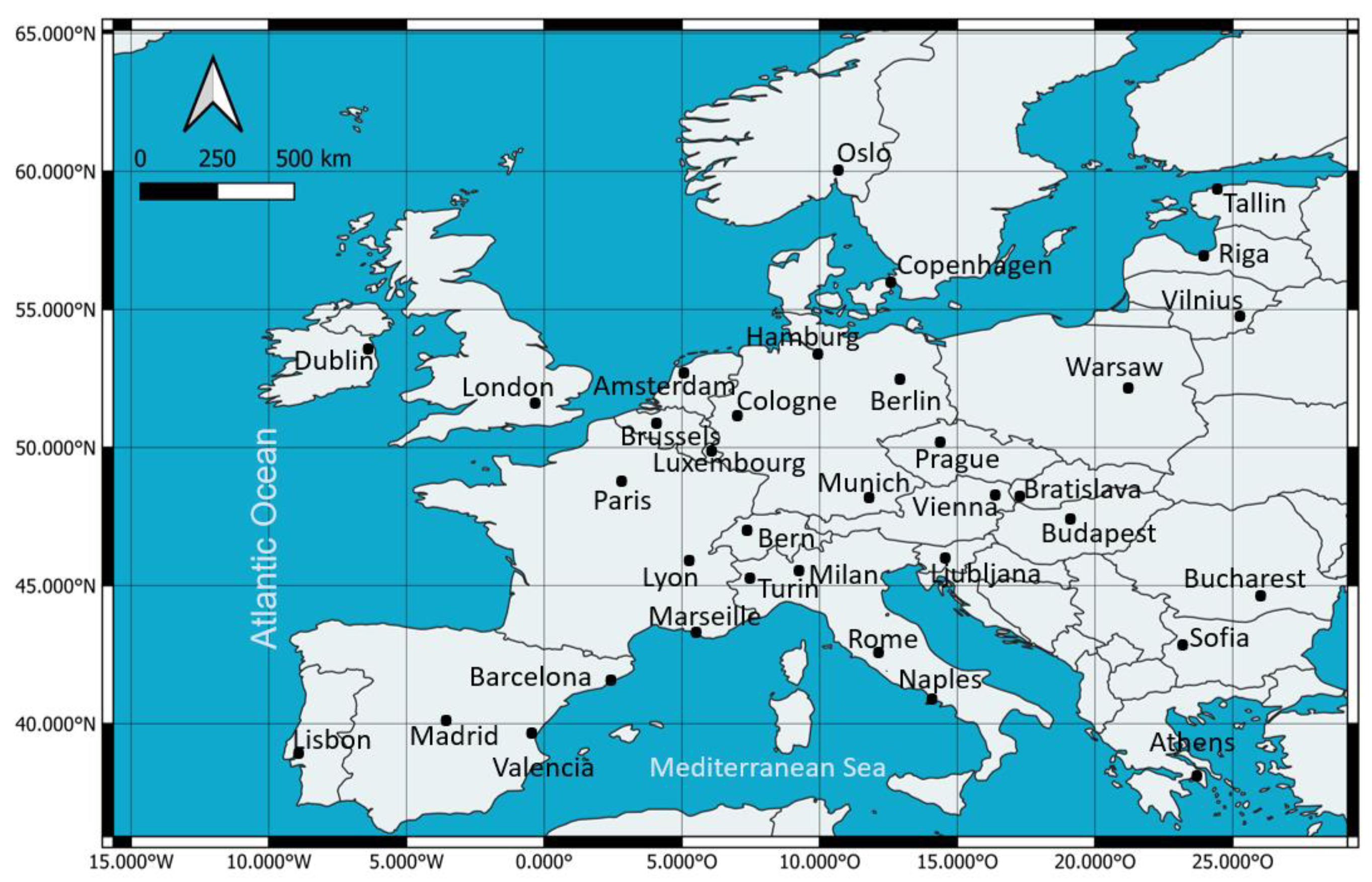
2.1. Investigation Period and Study Area

The investigation period covers the years 2015–2020. Special attention was paid to the period from 15 March 2020 to 30 April 2020, when the strict policies of the first lockdown in Europe stopped various anthropogenic activities nearly completely. The same period, i.e., 15 March to 30 April from 2015 to 2019, serves as reference data. A five-year baseline was chosen to minimize the impacts of inter-annual climatic variability. The study was carried out across Europe. Based on the data availability, it is possible to analyze a sample of 43 cities in Europe. The cities can be seen in Figure 1.

2.2. Air Pollutants under Study

For this study, the air pollutants NO2, O3, and PM2.5 were selected. Primary pollutants, i.e., directly emitted, such as NO2, are closely linked to human activity [15]. Thus, changes in air pollutant concentrations due to changes in anthropogenic behavior are expected. The main contributors to NO2 emissions in Europe are transport (39%) and energy production (16%), commercial, residential, and households (14%), and energy use in the industry (12%) [20]. Its lifetime in the atmosphere is between two to six hours in the summer daytime and 12 to 24 h during the winter and mainly depends on meteorology [26]. Due to its short lifetime, NO2 concentrations quickly alter when emissions change. In general, higher concentrations are found over densely populated cities, where emissions are higher than in the surrounding areas [15].
O3 is a secondary pollutant and is thus, unlike NO2, not directly emitted. It photochemically forms under solar radiation through chemical reactions of NOx and volatile organic compounds (VOCs) [18]. O3 emerges under solar radiation, thus unhealthy concentrations are predominantly yielded on sunny days [17]. In the winter, O3 concentrations are lower when NOx levels are usually high, and thus titration is intense [18]. The lifetime of O3 depends on meteorology and solar radiation—mainly on the chemistry of O3 itself, its oxidant level, and the NOx and VOCs—but on average, its lifetime in the troposphere is about 20–24 days [27].
PM2.5 can form through chemical reactions in the atmosphere, forming secondary PM. Sources can be from gaseous pollutants such as SO₂, ammonia, or NO2, especially due to power plants and combustion. On the other hand, it can be directly emitted in the form of dust, sea salt, smoke, trace elements, and crustal matter [14,17]. In Europe, the main anthropogenic contributors of PM2.5 are commercial, residential, and households (56%), industrial processes and product use (11%), agriculture (3%), road transport (11%), and energy use in industry (6%) [28].

2.3. Data

This study uses the LST data product from Terra and Aqua MODIS (MxD11A1 v6.1). The products are available from LP DAAC as gridded files. Its spatial resolution is 1 km. The sun-synchronous satellites traverse the equator at 10:30 and 13:30, respectively, local solar time, in the descending orbit and at 22:30 and 01:30 in the ascending orbit. The MxD11A1 data product provides the daily LST during the day- and night-time. The daily LST data are processed as explained in Sismanidis et al. [29], and the LST mean is calculated for each city (separately for the urban and the surrounding rural area).
From the LST, the SUHII is calculated by subtracting the rural arithmetic mean from the urban. The aim of calculating the SUHII is to reduce the noise and the existing variation in the data and make the signal from the changed human activities more pronounced. Because the diurnal and seasonal temperature cycle is higher than the expected magnitude of temperature differences between the lockdown period and the non-lockdown period, we normalized these differences to enhance the signal corresponding to the changed human activities. It must be noted that the SUHII also depends on the weather. However, by calculating the SUHII temperature variabilities throughout different years, the inter-annual variabilities and the magnitude of variations are reduced [30].
The air pollutant concentrations are from the Copernicus Atmosphere Monitoring Service (CAMS). The data assimilation embeds satellite and ground-based/in-situ observations and numerical models. The used product is the CAMS daily regional analysis. Here, one daily average value for each air pollutant is given per major European city [31].
Mobility data from Google’s COVID-19 Community Mobility Reports are used to examine how the number of visits to specific types of places changed during the COVID-19 lockdown in each city. We also use these data as a proxy for anthropogenic activity. There are six types of places, namely residences, transit stations, retail and recreation, grocery and pharmacy, workplaces, and parks. For residences, the percent change of average time spent at home is provided. The percentual change of one day for a specific place is related to a reference value for the respective weekday. The baseline data are the median value for each category and each weekday during the five-week period between January 3 and February 6 in 2020 before the lockdowns started. Thus, there are seven different reference values within a week [32].

2.4. Statistical Analysis

To quantify the changes between the lockdown and pre-COVID period, the data are split into two groups. The first group corresponds to the reference period (15 March to 30 April 2015–2019) and the second to the lockdown period of the first COVID-19 pandemic wave (15 March to 30 April 2020). For each variable, the percentage and the absolute difference between the two groups are computed.
To assess if the differences between the two groups are statistically significant, and to check whether the pre-COVID and lockdown values come from the same distribution a two-sample one-sided, a non-parametric Kolmogorov–Smirnov hypothesis test (KS-test) was carried out [33]. The significance level is α = 0.05 and the test hypotheses for all variables under study but ozone are the following:
  • H0: the two distributions are identical, F(x) ≥ G(x) for all x, where F(x) is the lockdown and G(x) is the reference period.
  • HA: they do not have the same distribution; the lockdown distributions are shifted toward lower values: F(x) < G(x) for at least one x.
Hypotheses for ozone:
  • H0, ozone: the two distributions are identical, F(x) ≤ G(x) for all x, where F(x) is the lockdown and G(x) is the reference period.
  • HA, ozone: they do not have the same distribution; the lockdown distributions are shifted toward higher values: F(x) > G(x) for at least one x.

3. Results

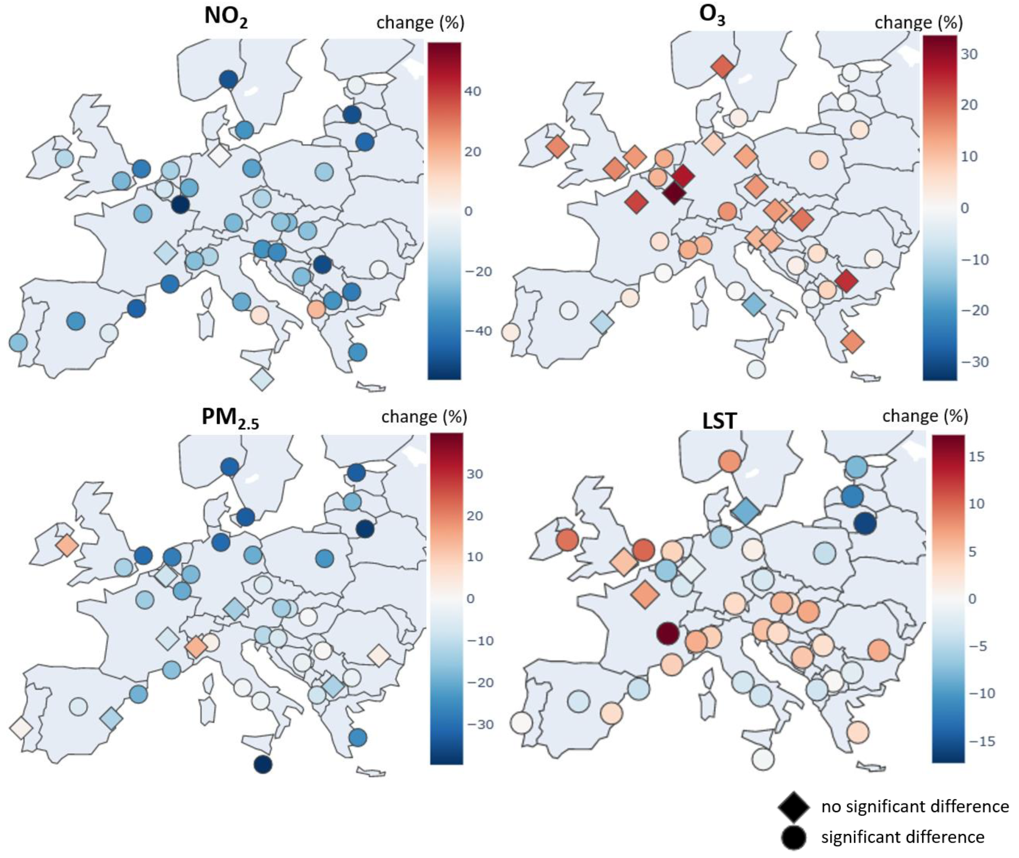
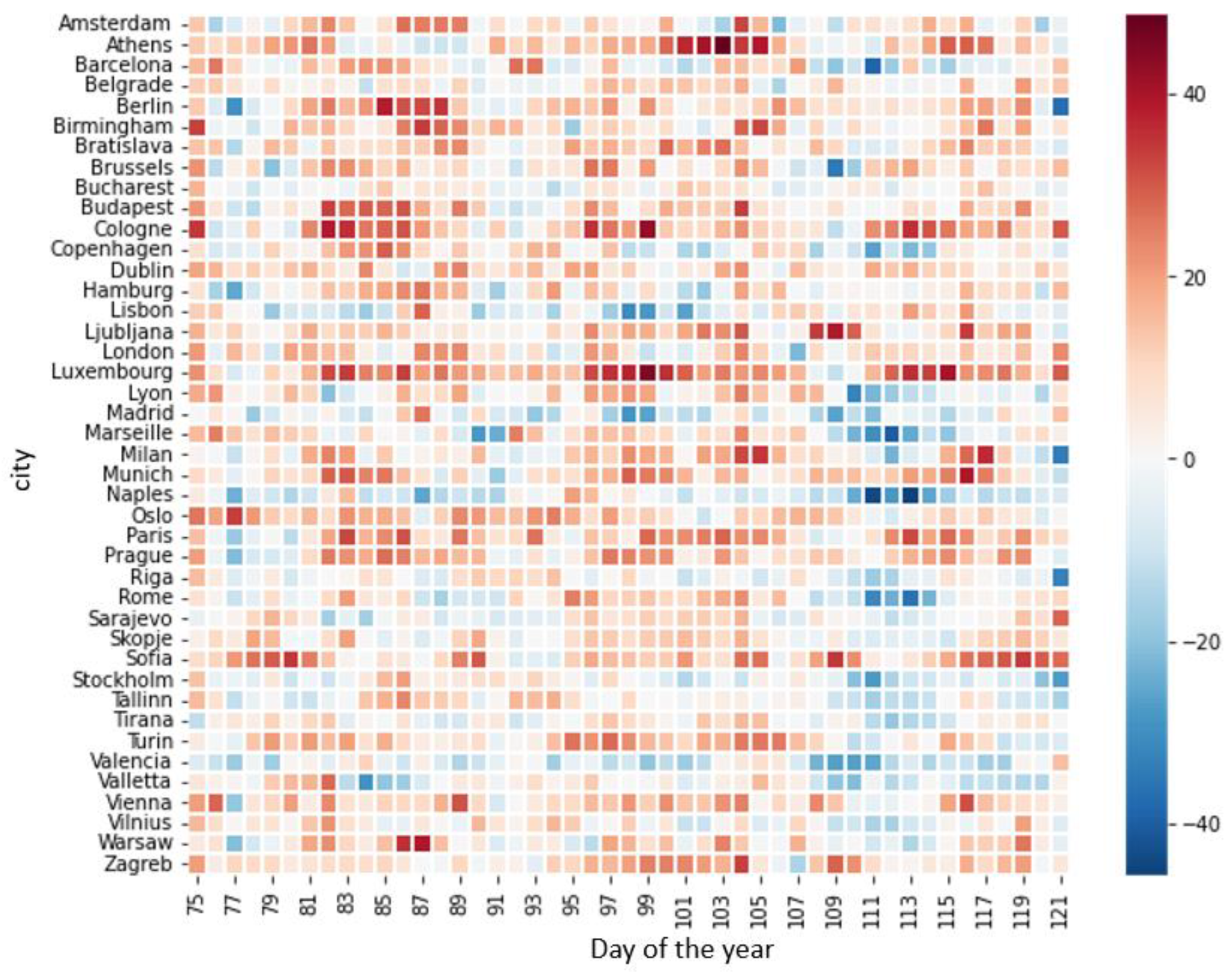
3.1. Multiparameter Overview

Figure 2 shows the results of the individual variables of the KS test combined with the relative change in 2020 compared with the reference period. For the KS test, in most cases, the null hypothesis can be rejected, i.e., the LST, NO2, and O3 differences between the lockdown and reference periods are statistically significant (shown with a circle). If there is no statistically significant change in the variable, this is indicated by a rhombus as a symbol. This is the case in Eastern Europe for the O3 values and the LST night-time values. For PM, the results are variable with no clear signal regarding the spatial distribution.
In general, a predominant decline in ground-level NO2 was recorded. Although most of the cities showed the same signals, the magnitude of change differed city-wise. The three cities with the largest percentual NO2 reductions are Luxembourg (−54.0% relative change, −12.3 µg/m3 absolute change), Riga (−50.7%, −5.1 µg/m3), and Belgrade (−50.4%, −6.8 µg/m3). Hamburg (+10.5%, +1.1 µg/m3), Tirana (+18.4%, +0.7 µg/m3), and Naples (+11.9%, +1.7 µg/m3) show the largest positive anomalies. For O3, a widespread increase is evident. The largest positive anomalies are found in Luxembourg (+41.1%, +20.5 µg/m3), Cologne (+35%, +15.7 µg/m3), and Paris (+27.1%, +13.1 µg/m3). In contrast to the other cities, cities in the Iberian Peninsula, Italy, and southern France show lower O3 concentrations in 2020. The greatest changes correspond to Naples (−12.1%, −8.9 µg/m3), Valencia (−10.3%, −7.5 µg/m3), and Madrid (7.2%, −5.0 µg/m3). PM2.5 anomalies are inconsistent over space. They predominantly decreased in Northern Europe. Strongest reductions can be observed in Tallin (−38.4%, −2.9 μg/m3), Vilnius (−37.4%, −4.6 μg/m3), and Oslo (−28.8%, −2.8 μg/m3). The highest increases were observed for PM2.5 in Dublin (+43.9%, +1.5 μg/m3), Turin (+31.4%, +5.5 μg/m3), and Milan (+19.7%, +4.1 μg/m3).

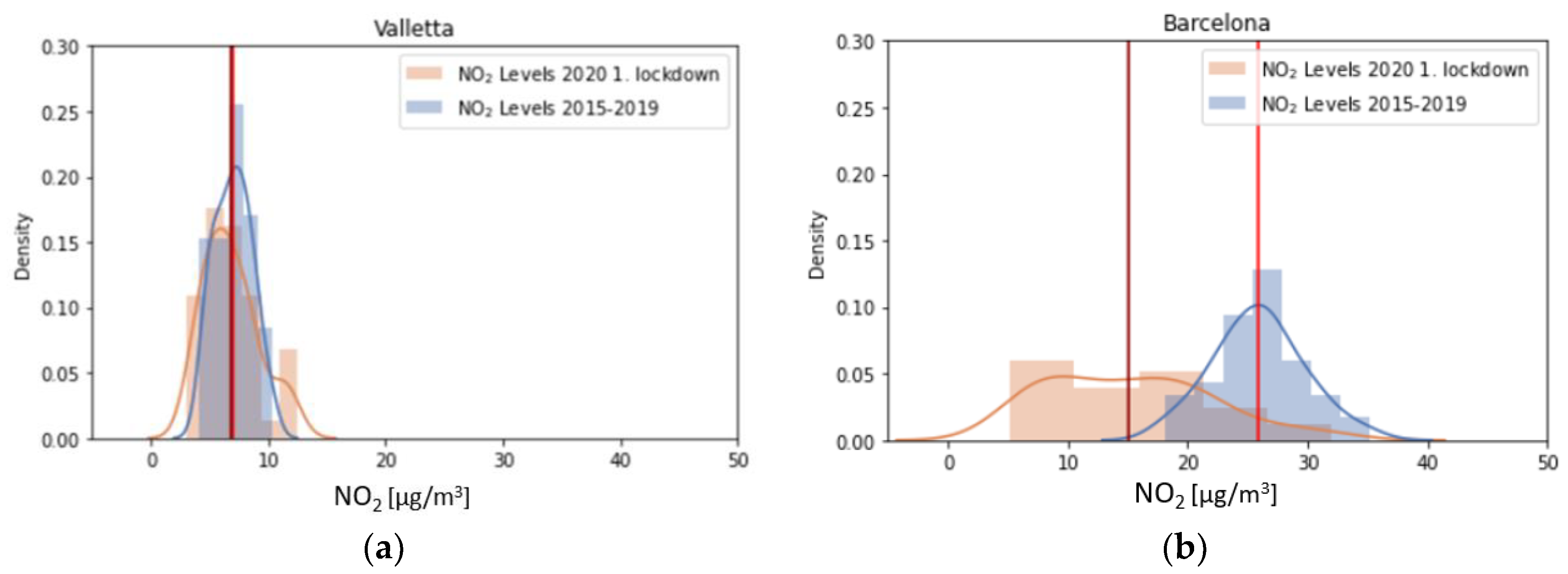
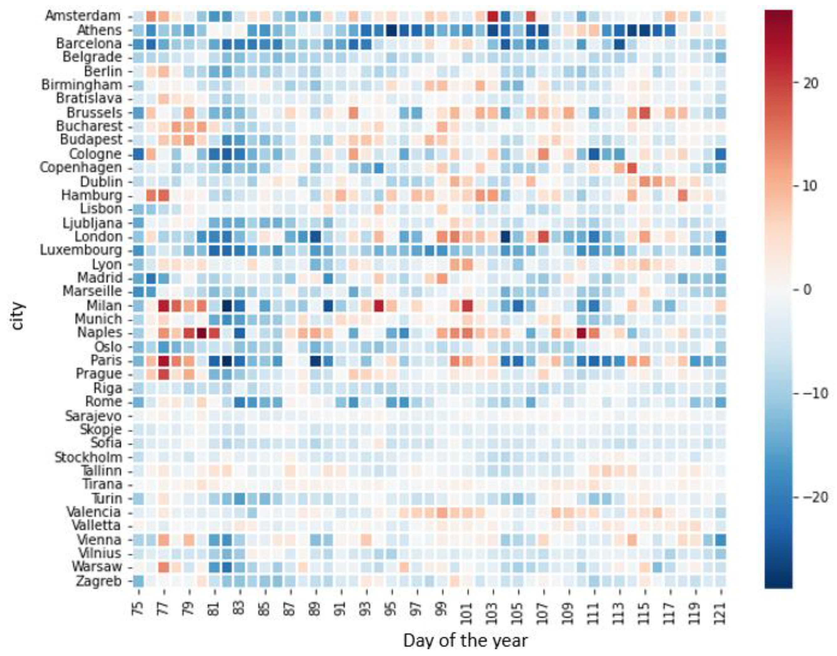
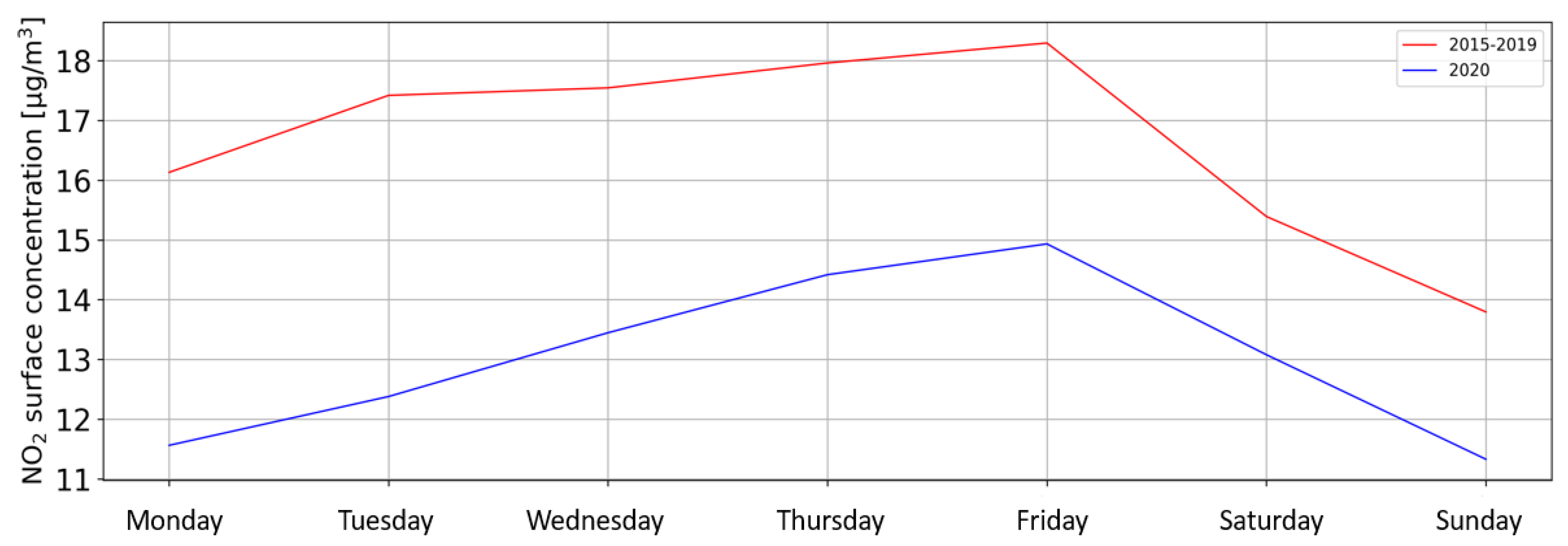
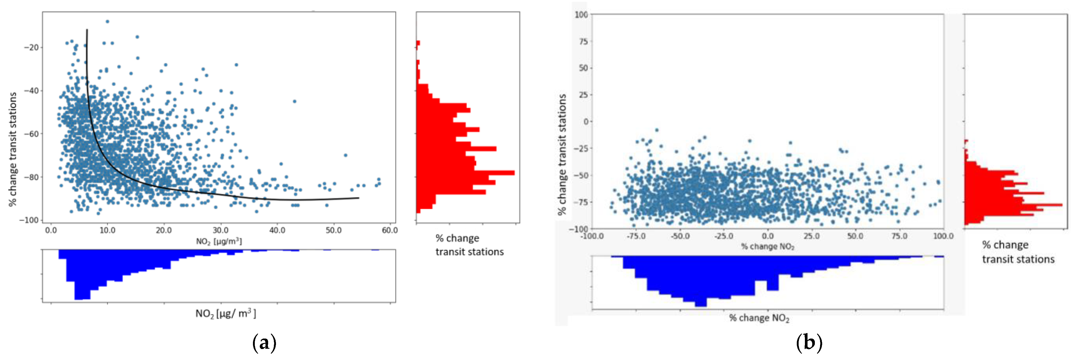
3.2. Nitrogen Dioxide
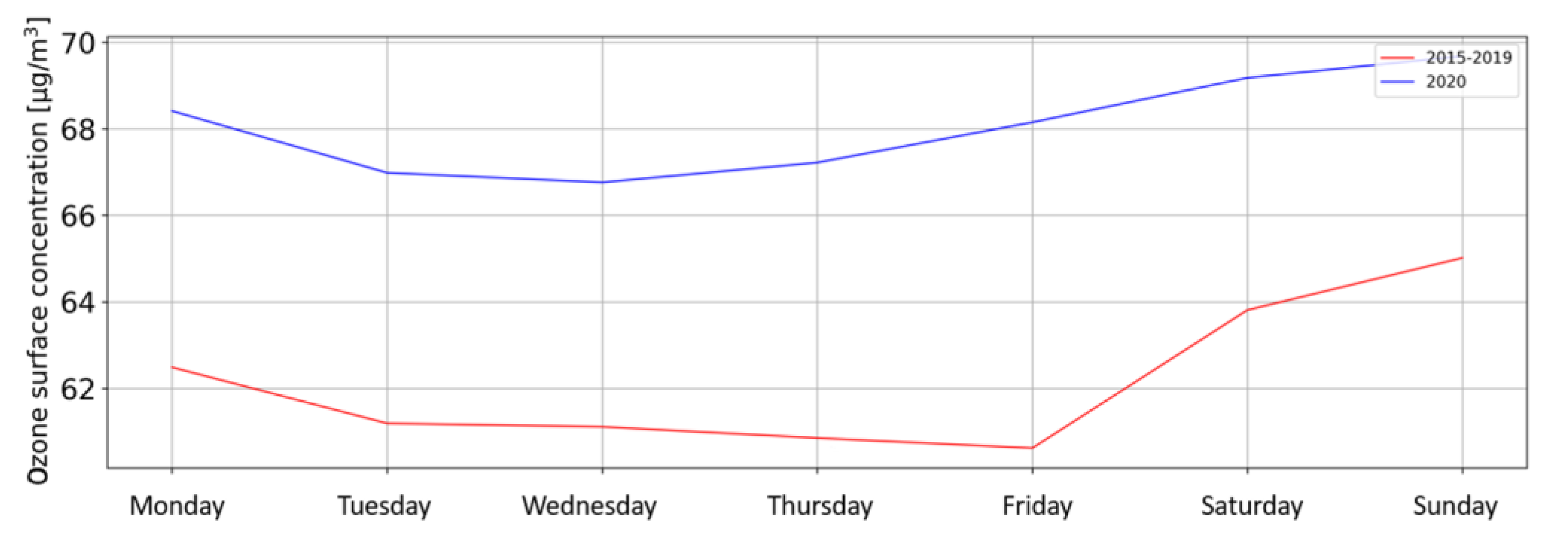
Figure 3 shows the change in the distribution of the daily NO2 levels averaged for all cities. Here, it is apparent that the mean of the NO2 concentration during the lockdown in 2020 (dark red line) and the binned observations for the individual concentrations are left-shifted, which means that they have decreased. Furthermore, the density is reduced as well, which underlines the flatter continuous density curve for 2020. The density is calculated by dividing the frequency by the class width. Thus, it represents the frequency per unit for the data in each class. At this point, it must be emphasized that the individual cities differ a lot. For some cities (such as Barcelona), the change is high, and in others (such as Valetta), the change is low (Figure 4).
The anomalies over the curfew period are shown in more detail in Figure 5. Here, the differences for each day and city are shown compared with the values for each city in the reference period. In general, the changes in the Eastern European and Scandinavian cities are rather small. It is noticeable that there is almost no NO2 concentration difference in Sarajevo. In contrast, much lower NO2 concentrations in 2020 (i.e., a strong negative anomaly) can be seen in Athens and Luxembourg. Some cities show inconsistent behavior, such as Brussels, London, Milan, or Paris. On the other hand, Hamburg, Tirana, and Naples predominantly show a positive change in NO2 concentrations compared with the reference period. Considering all cities, strong concentration declines in 2020 from day 81 of the year (22 March) approximately until day 91 (1 April) are noticeable. Thereon, several cities show concentration increases compared with the reference period, interrupted again by negative anomalies during days 104–106 of the year (14–16 April).
Looking at the average weekly pattern of all cities (Figure 6), the absolute NO2 concentrations are not only lower but the pattern itself changed. In general, measured NO2 concentrations increased, peaking on Fridays, and decreased towards the weekend. A comparatively stronger increase in concentrations from Monday to Friday can be seen in 2020 (~3.5 µg/m3 in 2020 vs. ~2 µg/m3 in the reference period). On Sundays and Mondays, the concentrations are the same in 2020. In contrast, in the reference period, higher concentrations on Mondays compared with Sundays are observed.

3.3. Ozone

Examining the O3 anomalies over the whole period, lower concentrations seem to prevail at the beginning of the lockdown. Around days 80 to 90 of the year (22 March–31 March), however, almost all cities show an increase in O3 concentration (Figure 7). Very striking is the strong increase in Athens, Budapest, Cologne, and Luxembourg. This is followed by a phase that tends to have less O3 in 2020 that lasts until day 95 (5 April). Until day 108 (18 April), most cities show higher O3 concentrations than in the reference period. The cities Lyon, Marseille, Naples, Rome, Madrid, and Valencia show strong negative anomalies, especially towards the end of the study period from day 109 (19 April).
In addition to the fact that surface O3 concentrations are mostly higher in 2020, concentrations tend to be higher on weekends (Figure 8). The pattern itself in 2020 compared with the reference period is similar. However, there is a smaller concentration increase in 2020 (~1.9 µg/m3) towards the weekend than in 2015–2019 (~4.2 µg/m3). In addition, O3 concentrations decrease in the reference period from Monday to Friday, whereas for 2020, they do so only until Wednesday. Further, the pattern is inverse in comparison to NO2.

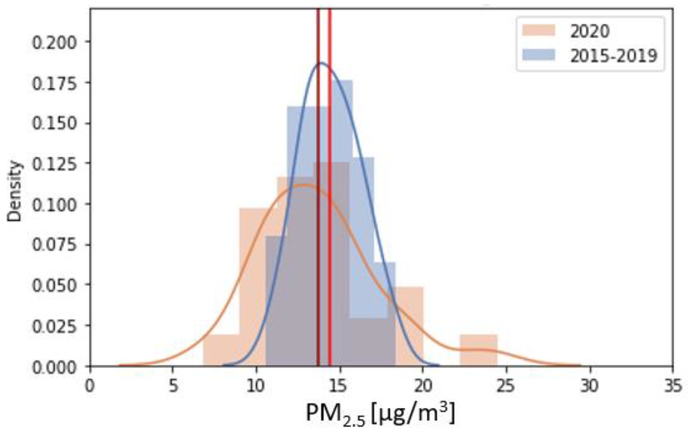
3.4. Particulate Matter

PM2.5 shows only a small shift in the mean concentration (Figure 9). Looking at the histograms, the bins are distributed in a greater range in 2020. Thus, both observations with higher and also with lower daily values are recorded in 2020, even though it has a comparatively lower density curve. The anomalies are not only inconsistent over space but also over time (Figure 10). However, it is noticeable that between days 77 and 80 (18 March–21 March), in some cities, there was a simultaneous increase in PM levels in 2020, followed by a drop until approximately day 86 (27 March). From day 87, with a few exceptions (e.g., Valetta, Naples), there was a positive anomaly that lasted about three days.

3.5. Land Surface Temperature
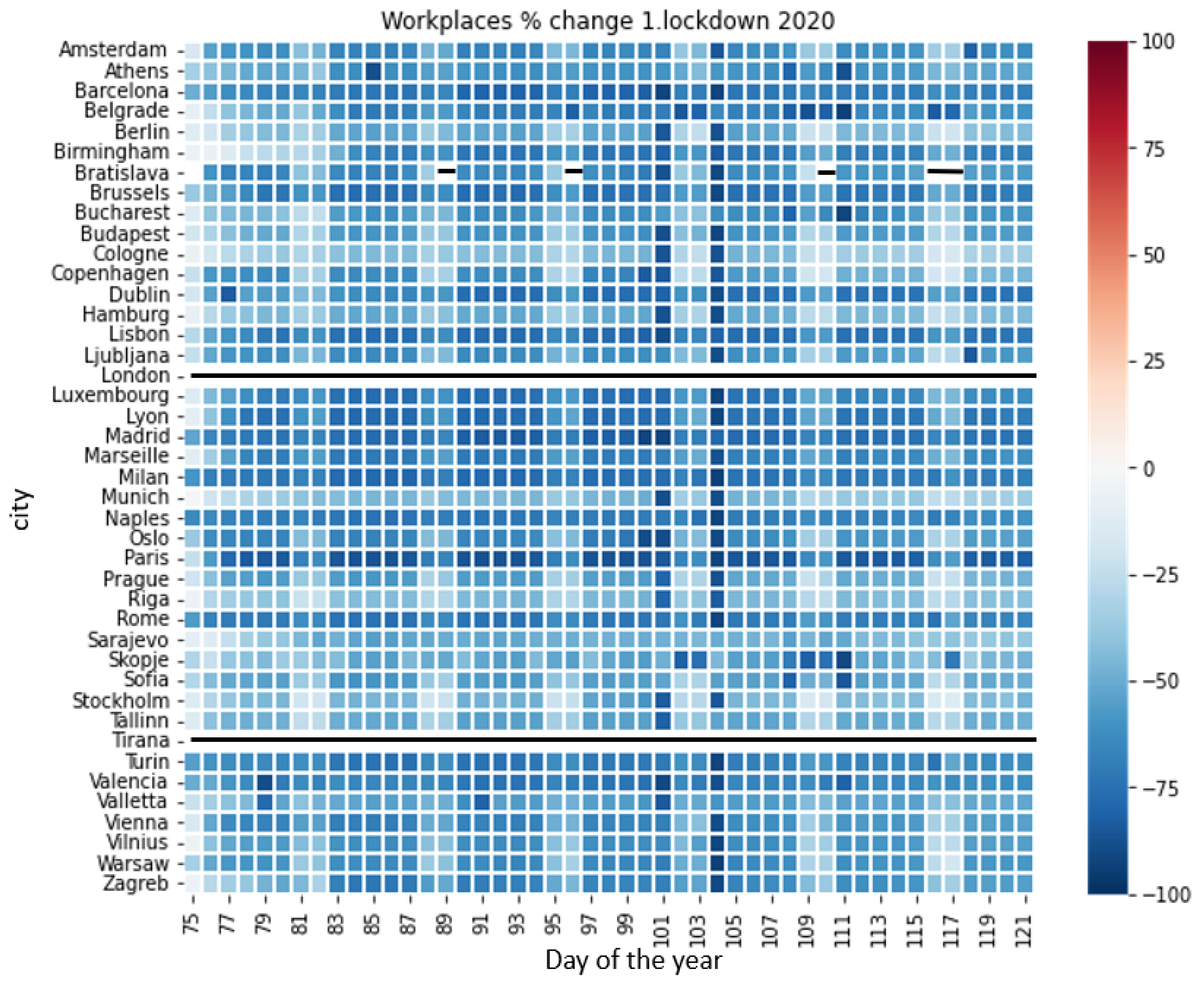
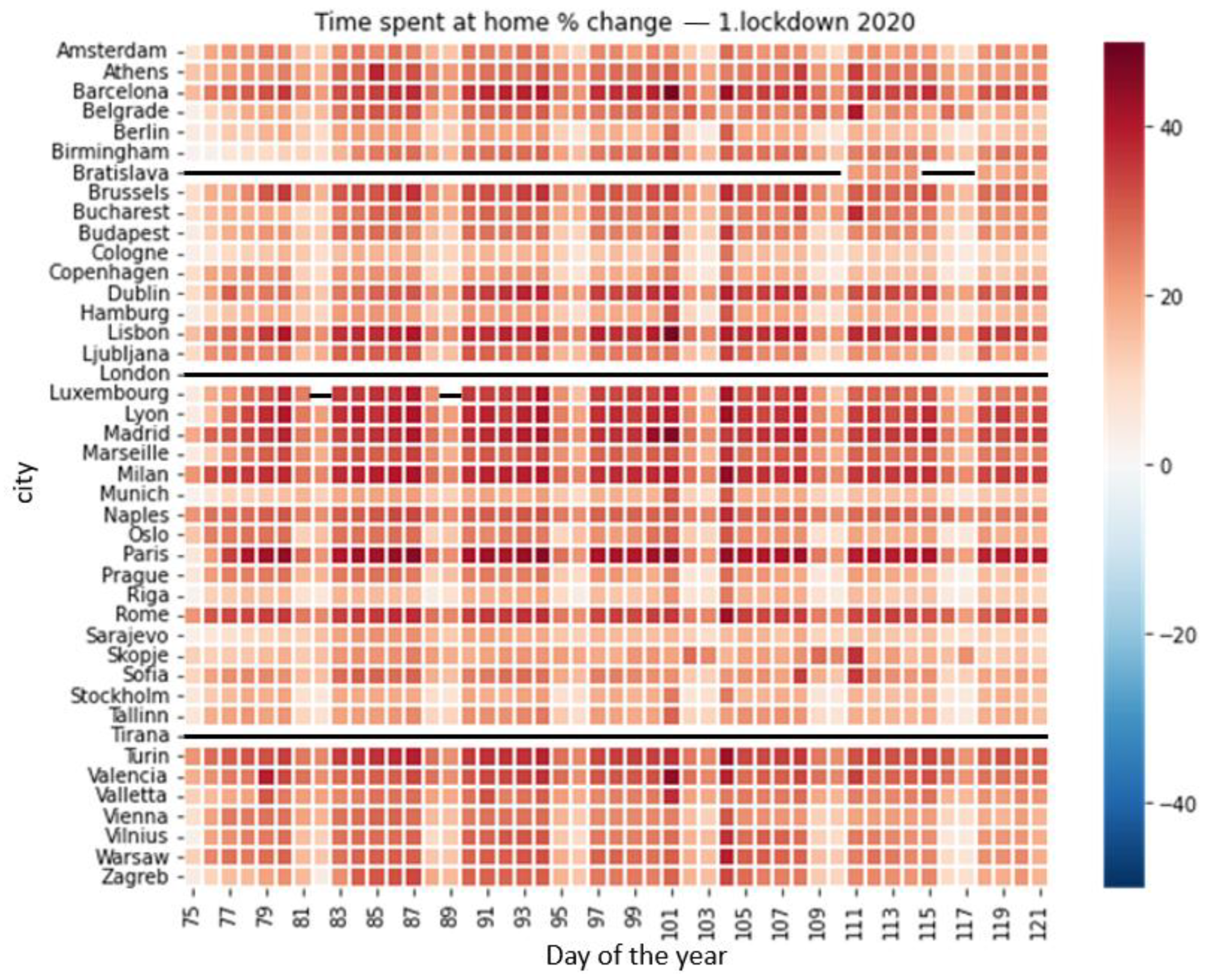
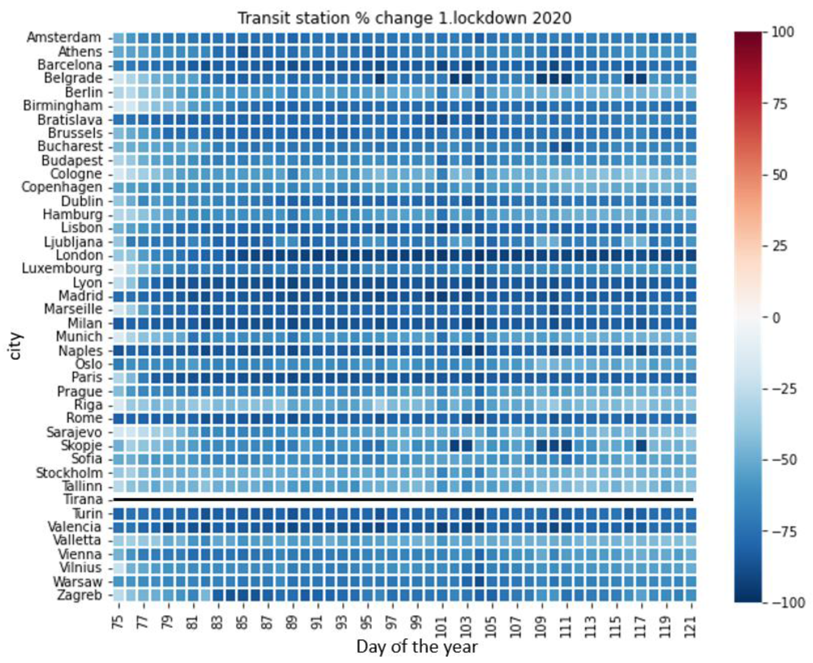
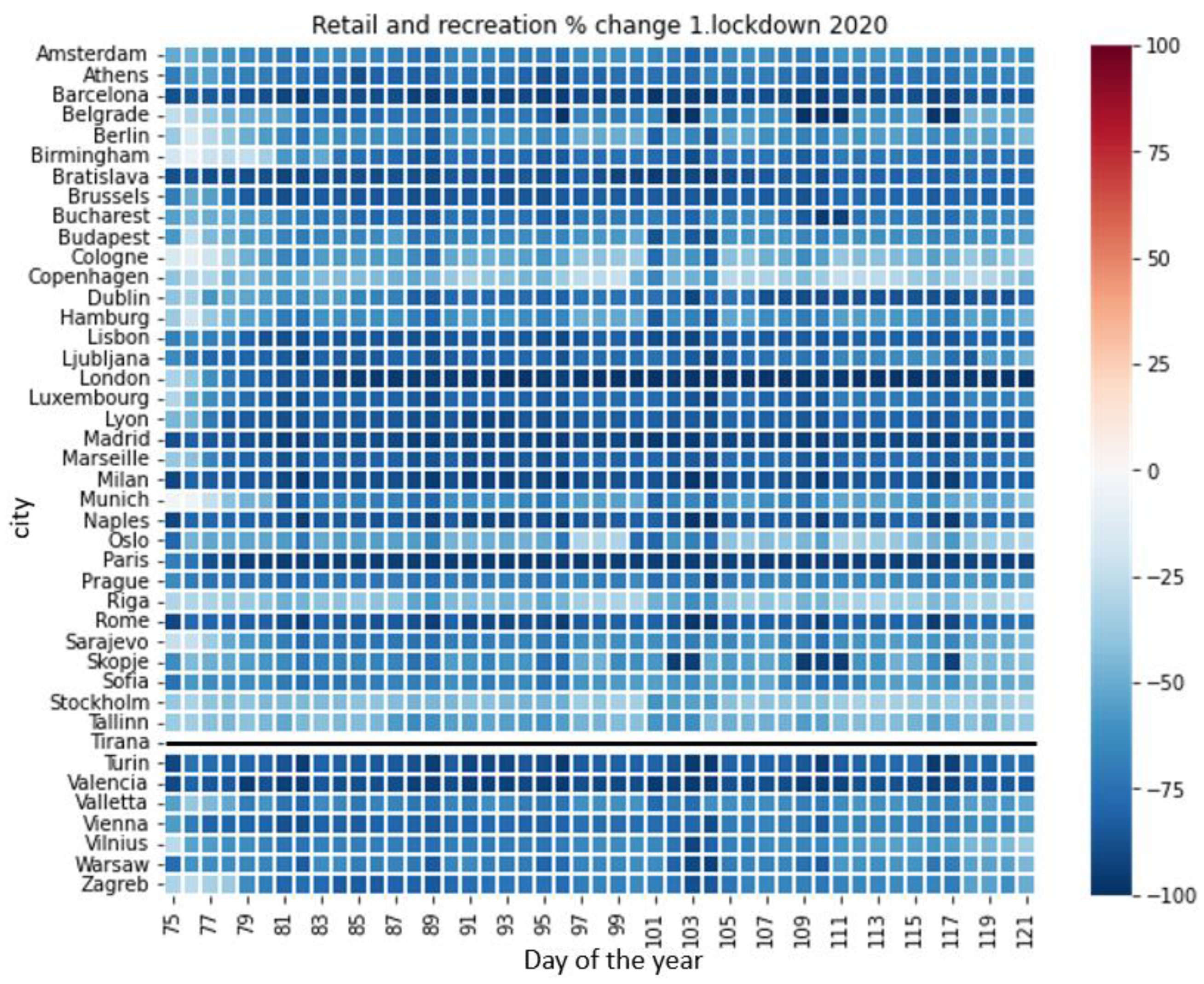
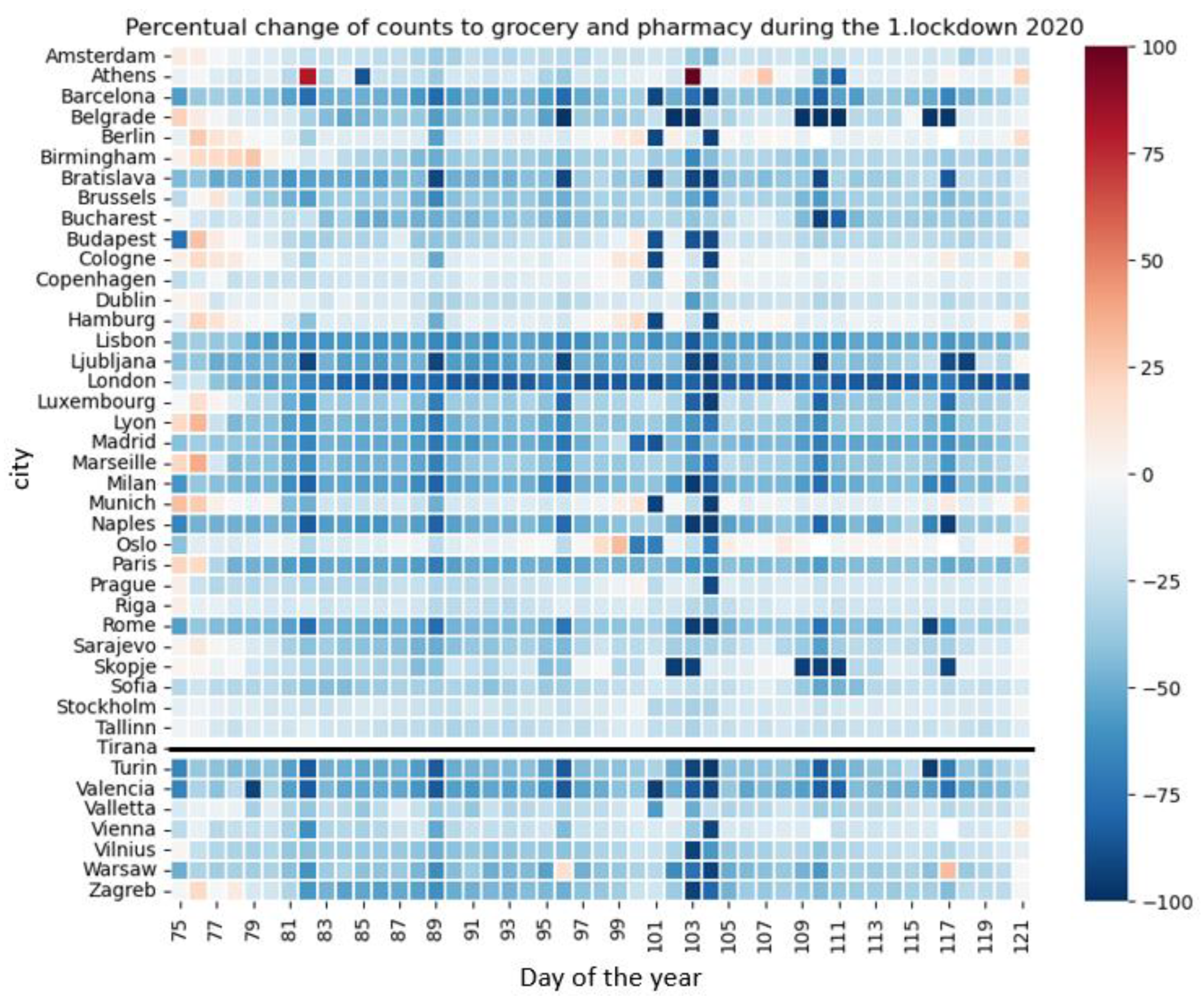
For both LST and SUHII, there is no clear signal of change (Figure 11). In total, there was only a very slight LST and SUHII reduction. Uncorrected weather data show both higher and lower LST in 2020 compared with the reference period and strongly diverge temporally and spatially (Figure 12).

3.6. Mobility Data

Figure 13 shows the percentual change of anthropogenic mobility during the study period (red box: 15 March to 30 April 2020) and the time after the first lockdown in Madrid and Stockholm. The cities of Madrid and Stockholm were selected as examples of a strict lockdown and a lockdown with very few ordinances, respectively. Spain and Italy, in general, had the most stringent measures, while the government of Sweden imposed almost no restrictions [34]. Scandinavian and Baltic cities had less strict measures, which was also the case in Germany, where schools have been closed, but the industrial sector largely remained open [35].
After the restrictions were imposed in mid-March, mobility was clearly reduced. All categories were visited less, except for “residential” because more time was spent at home. In general, the greatest changes can be observed in the categories of retail, recreation, and transit stations, and the least in parks, grocery, and pharmacy. After easing the restrictions, mobility gradually increased again, with parks being visited more than usual. It must be stated that the baseline is in February and that fewer parks are visited in winter than in summer anyway. However, mobility behavior has still not returned to the levels seen in the summer of 2020. Furthermore, the data show a weekly pattern. People were outside more and less at home on weekends but in total less than usual. Regarding the workplaces and transit stations, more people worked from home and did not use public transport. In contrast, on weekends, most of the employees do not work and changes are rather marginal. A detailed insight into how each mobility category changed in the individual cities can be seen in Appendix A.
Comparing the two cities, in Madrid, mobility was much more restricted, public life almost came to a halt, and thus mobility data show a greater decline. Transit stations, park visits, and retail and recreation had a change of almost −90%. Furthermore, significantly more time was spent at home. Buying groceries was the only allowed opportunity to leave the house [34]. In contrast, in Stockholm, the surplus of time spent at home was significantly lower (~+20%) than in Madrid (~+35%). In addition, changes at transit stations and workplaces were only about 50%. From the end of March and ongoing, parks were visited more than during the baseline period, reaching a maximum of +75%. At the beginning of June, the visits to parks considerably increased compared with the baseline in Stockholm (the large daily variations are because park visits are influenced by the weather conditions). Thus, the two exemplary selected cities clearly illustrate how different strictness levels are reflected in changes in mobility behavior.
In Figure 14, we examine how daily mobility is related to the variables under study, where each point corresponds to the value of one city on one day. As an example, the change in the number of visitors at transit stations is selected. The other categories follow the same pattern, except for “residential”, which shows an inversed pattern (not shown). The data distribution of the change in visitors at transit stations and the absolute NO2 values is clearly not linearly correlated (Figure 14a). Furthermore, it is useful to look not only at the absolute NO2 values, but also at the change in NO2 concentrations compared with the change at transit stations. The representation of the two allows inferences about how the NO2 values change related to the change in the number of visitors at transit stations. In Figure 14b, it can be seen that there were fewer people at transit stations and that the NO2 concentration has predominantly decreased during COVID-19. More importantly, it becomes evident that the change in visitors at transit stations has no visible influence on the NO2 change. Overall, we could not establish a clear relationship between mobility and the variables under study.

4. Discussion

4.1. Nitrogen Dioxide

In agreement with many other studies [15,19,21,36,37], strong reductions in NO2 levels in most European urban areas are observed. Regarding the weekly pattern of air pollutants, several studies depicted the same results as stated here. Masiol et al. [38] explain the pattern by arguing that less NO2 is emitted on weekends due to the fact that fewer people drive to work, and that heavy-duty vehicles are not allowed to drive on Sundays in most European cities. The pollutants accumulate within the week and reach their maximum on Friday because commuter traffic is reduced on weekends. For a distinct attribution to lockdown effects, improvements in air quality due to implemented measures should be taken into account. Some trend analysis of the five-year reference period of each city resulted in inconclusive results due to the high inter-annual variability and the comparably short period, and thus was not suitable to provide a consistent and robust estimate of the expected 2020 NO2 baseline concentrations for each city. The aggregated trend-based results paint a much clearer picture and agree with the mean-based analysis employed by this work. Overall, they too suggest that the NO2 concentration decreased but by a smaller magnitude (2.0 µg/m³ instead of 3.6 µg/m³). Thus, follow up studies should include post-2020 data to provide a better trend estimation and attribution. Moreover, weather effects should be eliminated, e.g., by using neural networks as suggested by [39]. Additional evidence for a lockdown-related signal is provided by the weekly cycle. The fact that NO2 concentrations are very similar on Mondays and Sundays in 2020 suggests that fewer people drove to work during the lockdown. On the contrary, under normal conditions, more emissions are emitted on Mondays than on weekends.

4.2. Ozone

The increase in O3 is related to the strong decline in NO2, a precursor of O3. Besides meteorological conditions, the ratio of NO2 and VOCs determines ozone production. If NO2 levels decrease, the VOC/NOx ratio is high, chemical titration with NO is reduced, and O3 levels increase. However, the response of O3 formation to changes in the VOC/NOx ratio is nonlinear [14,23,36,40]. The study of Shi et al. [40] states that reductions in traffic-related NO emissions lead to increases in O3 concentrations during the daytime. Further, they emphasize that sunny weather during the lockdown enhances the oxidizing process and leads to higher photochemical production of O3. However, possible divergences can be explained by the fact that O3 is regionally well-mixed and can be transported downwind, which can dominate local signals [36]. Thus, there is a high probability that the observed reductions of O3 in some cities such as Madrid, Valencia, or Naples can be attributed to meteorological processes.
The weekly O3 pattern can be indirectly attributed to human metabolism because of its chemical relationship to NO2. O3 shows the inverse pattern of NO2, i.e., an increase on weekends. This increase is observed in large parts of the world [16,41,42] and can be associated with a reduction in traffic, i.e., NO2 emissions, followed by a reduced titration of O3 [13,21]. However, in 2020 the changed human metabolism influenced the “business as usual” pattern and caused changes in the weekly variation of O3.

4.3. Particulate Matter

PM surface concentration changes are weak and inconsistent with no clear increase or decrease signals even within one city over the study period. Several studies partly corroborate these results and the lack of a geographical homogenous signal [36,40]. Strong variations can be expected because PM has various emission sources [43]; hence, no clear relationship between PM and traffic is found. On the one hand, reductions in primary emissions of PM and its precursors such as NO2 and VOCs emitted—for example from cars—led to declines. At the same time, the emissions from sectors such as agriculture, e.g., fertilizing, biomass combustion, waste burning, construction works, and industry, were not strongly affected by those measures. Especially in Western Europe, PM levels were high in early spring due to fertilizer spreading [36,44]. Furthermore, it must be considered that the lockdown took place in early spring, when air temperatures were still cool, and residential heating was necessary. With the surplus of time spent at home, heating in houses increased. In particular, wood burner stoves contribute to high PM levels [43,44]. Another reason for inconsistent signals in PM levels are local and regional meteorological conditions. PM levels can be influenced by temperature, humidity, precipitation, vertical mixing, and advection [25]. Moreover, regional and long-range air mass transport can significantly affect local PM concentrations positively or negatively [44]. For example, reductions in PM levels from road traffic can be overwhelmed by PM air mass transportation from more polluted regions [40]. All these factors counteracted the reductions in traffic and contributed to inconsistent signals. Finally, traffic-related measures to reduce harmful PM in cities had already been implemented within the EU before the lockdown started [43]. The fact that no strong changes in the PM levels were recorded can therefore also be due to previously taken measures that aimed to improve the air quality over the years.

4.4. Relationship of the Air Quality Variables and LST with Mobility Data

In contrast with other studies [45], we were not able to observe a clear relationship between the air pollutants, the LST, and the mobility variables, even though other works clearly attribute the NO2 declines to traffic depletion due to the stay-at-home order [14,15,46]. The transport sector is the largest contributor to NO2 emissions in Europe [28]. Thus, changes in surface NO2 levels serve as an indicator of altered human activities and local mobility. However, the results of this study indicate that the change in visitors at transit stations has no or only a low influence on NO2 emissions. Even though the results show that the number of visitors to transit stations has fallen significantly, this does not necessarily imply that fewer buses or trains operated, because timetables were likely maintained. This is also supported by Ropkins and Tate [47], which suggests that public transport in the UK, especially buses, did not stop during the lockdown. Therefore, air pollutants from this source remained close to pre COVID-19 levels. Nevertheless, the fact that a general decline in NO2 values was recorded may be due to great reductions in traffic with privately-owned cars and is not related to public transport. However, the mobility data only consider transit stations and public transport, not individual car driving.
The PM also shows a weak relationship with the mobility data. This is in line with the findings of Efe [48]. Even though some studies showed positive correlations between mobility and PM, attributing the drop in PM to traffic restrictions, e.g., [49], several studies obtained similar patterns to the ones observed here. For example, the study of Munir et al. [44] shows the same negative, weak correlation with PM2.5, although they only considered Northern England. They assumed that PM concentrations are primarily regulated by the weather and regional PM transportation than by traffic. Furthermore, in a dispersion modeling experiment in Sheffield, it becomes clear that PM emissions are mainly controlled by point sources and not by traffic [50]. The lockdown took place in spring when most households still used heating. Household heating is a substantial contributor to PM levels. This is especially relevant considering that people were ordered to stay at home as much as possible to combat the virus [36]. Shi et al. [40] illustrate in their study that PM2.5 shows a complex response to the lockdown measures. Road traffic makes a rather small contribution to PM. In contrast, secondary sources such as residential solid fuel use and industrial activity have a larger impact on PM levels. In addition, non-lockdown-affected sectors such as agriculture and livestock contribute to PM emissions [21,36]. Thus, changes in people’s mobility behavior do not always lead to reduced PM levels, because traffic is not the sole origin of PM.
Finally, it must be emphasized that there is no simple monocausality between air pollutants, temperature, and human mobility. There are several factors that have not been highlighted in this work such as meteorological conditions and chemical-physical reactions that influence the air pollutant levels. In fact, it would be too trivial to get a linear relationship between temperatures and air pollutants and the change in human activities, which depend very much on atmospheric conditions. Because the cities under study have very different microclimates, a simple derivation and inference to a single component are not possible.
Thus, it is crucial to include meteorological data in future analyses. Especially for temperature changes but also for air pollutant changes—in particular, O3—there remain open questions due to a dominating weather effect and the complexity of other meteorological and chemical factors, which must be revised in future work.

5. Conclusions

We investigated the changes and the relationships of air pollutants and LST with data describing the human activity in 43 European cities in the lockdown year of 2020 in comparison with the reference period 2015–2019. Our findings show that there are considerable spatial and temporal differences between cities and spatial patterns regarding the magnitude and even the direction of change. Coinciding with previous studies, the results depict reductions in anthropogenic activities such as visiting parks, transit stations, workplaces, or retail and recreation during the lockdown. Simultaneously, NO2 concentrations declined as much as −54% (in Luxemburg) compared with the reference period. In contrast, ozone levels increased, with the greatest relative changes also in Luxembourg (+41.1%). The O3 increase is attributed to a lower titration of O3 by NO due to the substantial decline in local NOx emissions. LST and PM spatially and temporally varied. Within our analysis, we depicted that some variables are more closely linked to human activity than others; the most pronounced is NO2. Here, especially human activity can be seen in the weekly cycle. The significant decreases in most cities are likely related to the lockdown, but for more specific attribution, additional analysis on trends and weather influences is envisaged. However, we were not able to attribute the changes to specific changes in mobility behavior. Many previous studies suggested that restrictions have a significant impact on anthropogenic activities and, correspondingly, on urban temperatures and air pollutants. Owing to the complexity of meteorological factors, open questions remain, especially regarding the change in SUHII and LST. Future work should aim to accurately capture the influence of prevailing weather patterns on temperature changes.

Author Contributions

Conceptualization, P.G., B.B. and P.S.; methodology, P.G., B.B. and P.S.; software, P.G.; validation, P.G.; formal analysis, P.G.; investigation, P.G.; resources, P.G. and P.S.; data curation, P.G. and P.S.; writing—original draft preparation, P.G.; writing—review and editing, P.S. and B.B.; visualization, P.G.; project administration, P.G. All authors have read and agreed to the published version of the manuscript.

Funding

This research received no external funding.

Data Availability Statement

The air quality data are openly available on Github at https://github.com/CopernicusAtmosphere/air-quality-covid19-response (accessed on 14 May 2023).

Acknowledgments

We thank Anne-Sophie Jesemann for supporting us with the time series analysis and interpretation of weather-related effects on NO2 concentrations.

Conflicts of Interest

The authors declare no conflict of interest.

Appendix A

Figure A1, Figure A2, Figure A3, Figure A4 and Figure A5 allow more detailed insight into the development of the alterations to Google’s COVID-19 Community Mobility Reports categories. Regarding workplace change, Figure A1 underlines that much fewer people drove to their workplaces. Further, it clearly emphasizes a weekend pattern, when fewer people work, leading to lesser changes. Equally, Figure A2 shows that more time was spent at home during the week. The two patterns are very similar but inverse to each other. The cities that had the largest negative changes in the workplace have the largest increase (positive change) in time spent at home. German cities, especially Cologne and Munich, had a comparatively lower change. This suggests that fewer citizens were in a home office but have continued to drive to work. In Germany, schools have been closed, but the industrial sector has remained largely open [35]. In addition, the Scandinavian and Baltic cities also show smaller changes. The change in French, Italian, and Spanish cities is particularly striking. They had the greatest negative alteration on workplace changes and the greatest positive on time spent at home. This underlines the severity of the enacted lockdown measures, where citizens were not allowed to drive to work and had to work from home. The two other mobility classes also fit in the spatial pattern of alterations. However, the intensities of change slightly differ. Temporally, the weekend–weekday pattern is not as pronounced as in Figure A1 and Figure A2. For the change of visitors to groceries and pharmacy (Figure A5), a weekly pattern is evident, caused by shops being closed on Sundays. In agreement with the above, German and North European cities showed minor declines. The strong decrease around days-of-year 102 and 103 coincides with the Eastern holidays when stores are closed.
Figure A1. Percentual workplace change compared from the reference period in 2015–2019 to the first lockdown in 2020.
Atmosphere 14 01025 g0a1
Figure A2. Percentual change of time spent at home compared from the reference period in 2015–2019 to the first lockdown in 2020.
Atmosphere 14 01025 g0a2
Figure A3. Percentual change of visitors at transit stations compared from the reference period in 2015–2019 to the first lockdown in 2020.
Atmosphere 14 01025 g0a3
Figure A4. Percentual change of visitors to retail and recreation compared from the reference period in 2015–2019 to the first lockdown in 2020.
Atmosphere 14 01025 g0a4
Figure A5. Percentual change of visitors to retail and recreation compared from the reference period in 2015–2019 to the first lockdown in 2020.
Atmosphere 14 01025 g0a5

References

  1. World Health Organization. Report of the WHO—China Joint Mission on Coronavirus Disease 2019 (COVID-19). Available online: https://www.who.int/publications-detail-redirect/report-of-the-who-china-joint-mission-on-coronavirus-disease-2019-(covid-19) (accessed on 18 August 2022).
  2. World Health Organization. Coronavirus. Available online: https://www.who.int/health-topics/coronavirus (accessed on 10 November 2022).
  3. World Health Organization. WHO Coronavirus (COVID-19) Dashboard. Available online: https://covid19.who.int (accessed on 18 August 2022).
  4. Le Quéré, C.; Jackson, R.B.; Jones, M.W.; Smith, A.J.P.; Abernethy, S.; Andrew, R.M.; De-Gol, A.J.; Willis, D.R.; Shan, Y.; Canadell, J.G.; et al. Temporary Reduction in Daily Global CO2 Emissions during the COVID-19 Forced Confinement. Nat. Clim. Change 2020, 10, 647–653. [Google Scholar] [CrossRef]
  5. Anania, J.; Mello, B.A.; de Angrist, N.; Barnes, R.; Boby, T.; Cavalieri, A.; Edwards, B.; Webster, S.; Ellen, L.; Furst, R.; et al. Variation in Government Responses to COVID-19; Blavatnik School Government Work Paper; University of Oxford: Oxford, UK, 2022. [Google Scholar]
  6. Metya, A.; Dagupta, P.; Halder, S.; Chakraborty, S.; Tiwari, Y.K. COVID-19 Lockdowns Improve Air Quality in the South-East Asian Regions, as Seen by the Remote Sensing Satellites. Aerosol Air Qual. Res. 2020, 20, 1772–1782. [Google Scholar] [CrossRef]
  7. Jin, M.; Dickinson, R.E. Land Surface Skin Temperature Climatology: Benefitting from the Strengths of Satellite Observations. Environ. Res. Lett. 2010, 5, 044004. [Google Scholar] [CrossRef] [Green Version]
  8. Oke, T.R.; Mills, G.; Christen, A.; Voogt, J.A. Urban Climates; Oke, T.R., Ed.; Cambridge University Press: Cambridge, UK, 2017; ISBN 978-0-521-84950-0. [Google Scholar]
  9. Liu, Z.; Lai, J.; Zhan, W.; Bechtel, B.; Voogt, J.; Quan, J.; Hu, L.; Fu, P.; Huang, F.; Li, L.; et al. Urban Heat Islands Significantly Reduced by COVID-19 Lockdown. Geophys. Res. Lett. 2022, 49, e2021GL096842. [Google Scholar] [CrossRef]
  10. Hadibasyir, H.Z.; Rijal, S.S.; Sari, D.R. Comparison of Land Surface Temperature during and before the Emergence of COVID-19 Using Modis Imagery in Wuhan City, China. Forum Geogr. 2020, 34, 1–15. [Google Scholar] [CrossRef]
  11. Parida, B.R.; Bar, S.; Kaskaoutis, D.; Pandey, A.C.; Polade, S.D.; Goswami, S. Impact of COVID-19 Induced Lockdown on Land Surface Temperature, Aerosol, and Urban Heat in Europe and North America. Sustain. Cities Soc. 2021, 75, 103336. [Google Scholar] [CrossRef] [PubMed]
  12. Taoufik, M.; Laghlimi, M.; Fekri, A. Comparison of Land Surface Temperature Before, During and After the COVID-19 Lockdown Using Landsat Imagery: A Case Study of Casablanca City, Morocco. Geomat. Environ. Eng. 2021, 15, 105–120. [Google Scholar] [CrossRef]
  13. García, D.H.; Díaz, J.A. Impacts of the COVID-19 Confinement on Air Quality, the Land Surface Temperature and the Urban Heat Island in Eight Cities of Andalusia (Spain). Remote Sens. Appl. Soc. Environ. 2022, 25, 100667. [Google Scholar] [CrossRef]
  14. Adam, M.G.; Tran, P.T.; Balasubramanian, R. Air Quality Changes in Cities during the COVID-19 Lockdown: A Critical Review. Atmos. Res. 2021, 264, 105823. [Google Scholar] [CrossRef] [PubMed]
  15. Barré, J.; Petetin, H.; Colette, A.; Guevara, M.; Peuch, V.-H.; Rouil, L.; Engelen, R.; Inness, A.; Flemming, J.; García-Pando, C.P.; et al. Estimating Lockdown-Induced European NO2 Changes Using Satellite and Surface Observations and Air Quality Models. Atmos. Chem. Phys. 2021, 21, 7373–7394. [Google Scholar] [CrossRef]
  16. Sicard, P.; De Marco, A.; Agathokleous, E.; Feng, Z.; Xu, X.; Paoletti, E.; Rodriguez, J.J.D.; Calatayud, V. Amplified Ozone Pollution in Cities during the COVID-19 Lockdown. Sci. Total Environ. 2020, 735, 139542. [Google Scholar] [CrossRef]
  17. NASA. Earth Science Data Systems Health and Air Quality Data Pathfinder. Available online: http://www.earthdata.nasa.gov/learn/pathfinders/health-and-air-quality-data-pathfinder (accessed on 18 August 2022).
  18. Wijnands, J.S.; Nice, K.A.; Seneviratne, S.; Thompson, J.; Stevenson, M. The Impact of the COVID-19 Pandemic on Air Pollution: A Global Assessment Using Machine Learning Techniques. Atmos. Pollut. Res. 2022, 13, 101438. [Google Scholar] [CrossRef] [PubMed]
  19. Zhang, Z.; Arshad, A.; Zhang, C.; Hussain, S.; Li, W. Unprecedented Temporary Reduction in Global Air Pollution Associated with COVID-19 Forced Confinement: A Continental and City Scale Analysis. Remote Sens. 2020, 12, 2420. [Google Scholar] [CrossRef]
  20. European Space Agency. Air Pollution Remains Low as Europeans Stay at Home. Available online: https://www.esa.int/Applications/Observing_the_Earth/Copernicus/Sentinel-5P/Air_pollution_remains_low_as_Europeans_stay_at_home (accessed on 18 August 2022).
  21. Tobías, A.; Carnerero, C.; Reche, C.; Massagué, J.; Via, M.; Minguillón, M.C.; Alastuey, A.; Querol, X. Changes in Air Quality during the Lockdown in Barcelona (Spain) One Month into the SARS-CoV-2 Epidemic. Sci. Total Environ. 2020, 726, 138540. [Google Scholar] [CrossRef] [PubMed]
  22. He, G.; Pan, Y.; Tanaka, T. The Short-Term Impacts of COVID-19 Lockdown on Urban Air Pollution in China. Nat. Sustain. 2020, 3, 1005–1011. [Google Scholar] [CrossRef]
  23. Nichol, J.E.; Bilal, M.; Ali, A.; Qiu, Z. Air Pollution Scenario over China during COVID-19. Remote Sens. 2020, 12, 2100. [Google Scholar] [CrossRef]
  24. Alqasemi, A.S.; Hereher, M.E.; Kaplan, G.; Al-Quraishi, A.M.F.; Saibi, H. Impact of COVID-19 Lockdown upon the Air Quality and Surface Urban Heat Island Intensity over the United Arab Emirates. Sci. Total Environ. 2021, 767, 144330. [Google Scholar] [CrossRef]
  25. Venter, Z.S.; Aunan, K.; Chowdhury, S.; Lelieveld, J. COVID-19 Lockdowns Cause Global Air Pollution Declines. Proc. Natl. Acad. Sci. USA 2020, 117, 18984–18990. [Google Scholar] [CrossRef]
  26. Beirle, S.; Boersma, K.F.; Platt, U.; Lawrence, M.G.; Wagner, T. Megacity Emissions and Lifetimes of Nitrogen Oxides Probed from Space. Science 2011, 333, 1737–1739. [Google Scholar] [CrossRef]
  27. Elshorbany, Y.F.; Kleffmann, J.; Kurtenbach, R.; Rubio, M.; Lissi, E.; Villena, G.; Gramsch, E.; Rickard, R.; Pilling, M.J.; Wiesen, P. Summertime Photochemical Ozone Formation in Santiago, Chile. Atmos. Environ. 2009, 43, 6398–6407. [Google Scholar] [CrossRef]
  28. European Environment Agency. European Union Emission Inventory Report 1990–2018 under the UNECE Convention on Long-Range Transboundary Air Pollution (LRTAP); European Environment Agency Publications Office: Copenhagen, Denmark, 2020.
  29. Sismanidis, P.; Bechtel, B.; Perry, M.; Ghent, D. The Seasonality of Surface Urban Heat Islands across Climates. Remote Sens. 2022, 14, 2318. [Google Scholar] [CrossRef]
  30. Stewart, I.D.; Oke, T.R. Local Climate Zones for Urban Temperature Studies. Bull. Am. Meteorol. Soc. 2012, 93, 1879–1900. [Google Scholar] [CrossRef]
  31. CAMS. European Air Quality Information in Support of the COVID-19 Crisis|Copernicus. Available online: https://atmosphere.copernicus.eu/european-air-quality-information-support-covid-19-crisis (accessed on 18 August 2022).
  32. Google LLC. COVID-19 Community Mobility Report. Available online: https://www.google.com/covid19/mobility?hl=en-GB (accessed on 18 August 2022).
  33. Gao, X. Nonparametric Statistics. In Encyclopedia of Research Design; Salkind, N.J., Ed.; SAGE Publications Ltd.: Thousand Oaks, CA, USA, 2010; pp. 915–920. [Google Scholar]
  34. Codagnone, C.; Bogliacino, F.; Gómez, C.; Folkvord, F.; Liva, G.; Charris, R.; Montealegre, F.; Villanueva, F.L.; Veltri, G.A. Restarting “Normal” Life after COVID-19 and the Lockdown: Evidence from Spain, the United Kingdom, and Italy. Soc. Indic. Res. 2021, 158, 241–265. [Google Scholar] [CrossRef]
  35. Fairless, T. How Germany Kept Its Factories Open during the Pandemic. The Wall Street Journal, 6 May 2020. Available online: https://br.advfn.com/noticias/DJN/2020/artigo/82392711(accessed on 27 April 2023).
  36. Menut, L.; Bessagnet, B.; Siour, G.; Mailler, S.; Pennel, R.; Cholakian, A. Impact of Lockdown Measures to Combat COVID-19 on Air Quality over Western Europe. Sci. Total Environ. 2020, 741, 140426. [Google Scholar] [CrossRef] [PubMed]
  37. Rossi, R.; Ceccato, R.; Gastaldi, M. Effect of Road Traffic on Air Pollution. Experimental Evidence from COVID-19 Lockdown. Sustainability 2020, 12, 8984. [Google Scholar] [CrossRef]
  38. Masiol, M.; Squizzato, S.; Formenton, G.; Harrison, R.M.; Agostinelli, C. Air Quality Across a European Hotspot: Spatial Gradients, Seasonality, Diurnal Cycles and Trends in the Veneto Region, NE Italy. Sci. Total Environ. 2017, 576, 210–224. [Google Scholar] [CrossRef] [PubMed]
  39. Jesemann, A.-S.; Matthias, V.; Böhner, J.; Bechtel, B. Using Neural Network NO2-Predictions to Understand Air Quality Changes in Urban Areas—A Case Study in Hamburg. Atmosphere 2022, 13, 1929. [Google Scholar] [CrossRef]
  40. Shi, Z.; Song, C.; Liu, B.; Lu, G.; Xu, J.; Van Vu, T.; Elliott, R.J.R.; Li, W.; Bloss, W.J.; Harrison, R.M. Abrupt But Smaller Than Expected Changes in Surface Air Quality Attributable to COVID-19 Lockdowns. Sci. Adv. 2021, 7, eabd6696. [Google Scholar] [CrossRef]
  41. Zou, Y.; Charlesworth, E.; Yin, C.; Yan, X.; Deng, X.; Li, F. The Weekday/Weekend Ozone Differences Induced by the Emissions Change during Summer and Autumn in Guangzhou, China. Atmos. Environ. 2019, 199, 114–126. [Google Scholar] [CrossRef]
  42. Adame, J.A.; Hernández-Ceballos, M.; Sorribas, M.; Lozano, A.; De la Morena, B.A. Weekend-Weekday Effect Assessment for O3, NOx, CO and PM10 in Andalusia, Spain (2003–2008). Aerosol Air Qual. Res. 2014, 14, 1862–1874. [Google Scholar] [CrossRef] [Green Version]
  43. Hörmann, S.; Jammoul, F.; Kuenzer, T.; Stadlober, E. Separating the Impact of Gradual Lockdown Measures on Air Pollutants from Seasonal Variability. Atmos. Pollut. Res. 2021, 12, 84–92. [Google Scholar] [CrossRef] [PubMed]
  44. Munir, S.; Coskuner, G.; Jassim, M.S.; Aina, Y.A.; Ali, A.; Mayfield, M. Changes in Air Quality Associated with Mobility Trends and Meteorological Conditions during COVID-19 Lockdown in Northern England, UK. Atmosphere 2021, 12, 504. [Google Scholar] [CrossRef]
  45. Shanableh, A.; Al-Ruzouq, R.; Khalil, M.A.; Gibril, M.B.A.; Hamad, K.; Alhosani, M.; Stietiya, M.H.; Bardan, M.; Mansoori, S.A.; Hammouri, N.A. COVID-19 Lockdown and the Impact on Mobility, Air Quality, and Utility Consumption: A Case Study from Sharjah, United Arab Emirates. Sustainability 2022, 14, 1767. [Google Scholar] [CrossRef]
  46. Hale, T.; Angrist, N.; Goldszmidt, R.; Kira, B.; Petherick, A.; Phillips, T.; Webster, S.; Cameron-Blake, E.; Hallas, L.; Majumdar, S.; et al. A Global Panel Database of Pandemic Policies (Oxford COVID-19 Government Response Tracker). Nat. Hum. Behav. 2021, 5, 529–538. [Google Scholar] [CrossRef] [PubMed]
  47. Ropkins, K.; Tate, J.E. Early Observations on the Impact of the COVID-19 Lockdown on Air Quality Trends Across the UK. Sci. Total Environ. 2020, 754, 142374. [Google Scholar] [CrossRef] [PubMed]
  48. Efe, B. Air quality Improvement and Its Relation to Mobility during COVID-19 Lockdown in Marmara Region, Turkey. Environ. Monit. Assess. 2022, 194, 255. [Google Scholar] [CrossRef] [PubMed]
  49. Gorrochategui, E.; Hernandez, I.; Pérez-Gabucio, E.; Lacorte, S.; Tauler, R. Temporal Air Quality (NO2, O3, and PM10) Changes in Urban and Rural Stations in Catalonia during COVID-19 Lockdown: An Association with Human Mobility and Satellite Data. Environ. Sci. Pollut. Res. 2022, 29, 18905–18922. [Google Scholar] [CrossRef]
  50. Munir, S.; Mayfield, M.; Coca, D.; Mihaylova, L.; Osammor, O. Analysis of Air Pollution in Urban Areas with Airviro Dispersion Model—A Case Study in the City of Sheffield, United Kingdom. Atmosphere 2020, 11, 285. [Google Scholar] [CrossRef] [Green Version]
Figure 1. Cities under study.
Atmosphere 14 01025 g001
Figure 2. Relative changes in 2020 compared with the reference period of 2015–2019 for NO2, O3, PM2.5, and LST combined with the KS test results. The circle means that there is a statistical significance (reject H0), i.e., the variable significantly altered during the lockdown period compared with the reference period. The rhomb indicates there is no significant change (accept H0) according to the KS test.
Atmosphere 14 01025 g002
Figure 3. Distribution of the NO2 levels [µg/m³] during lockdown and reference period averaged over all cities. The vertical line corresponds to the mean of the period, and the columns to the binned observations.
Atmosphere 14 01025 g003
Figure 4. Distribution of the daily NO2 levels [µg/m³] during lockdown and reference period for (a) Valetta and for (b) Barcelona.
Atmosphere 14 01025 g004
Figure 5. NO2 anomalies [µg/m3] (15 March–30 April 2020 vs. 15 March–30 April 2015–2019).
Atmosphere 14 01025 g005
Figure 6. Weekly mean NO2 [µg/m3] for all cities during 15 March–30 April in 2020 and the reference period.
Atmosphere 14 01025 g006
Figure 7. Ozone anomalies [µg/m3] (15 March–30 April 2020 vs. 15 March–30 April 2015–2019).
Atmosphere 14 01025 g007
Figure 8. Weekly mean ozone levels [µg/m3] for all cities 15 March–30 April in 2020 and 2015–2019.
Atmosphere 14 01025 g008
Figure 9. Distribution of the daily PM2.5 levels [µg/m³] averaged over all cities during lockdown and reference period.
Atmosphere 14 01025 g009
Figure 10. PM2.5 anomalies [µg/m3] (15 March–30 April 2020 vs. 15 March–30 April 2015–2019).
Atmosphere 14 01025 g010
Figure 11. Distribution of the (a) LST [°C] and (b) SUHII [K] averaged over all cities during lockdown and reference period.
Atmosphere 14 01025 g011
Figure 12. (a) LST [°C] and (b) SUHII [K] anomalies (15 March–30 April 2020 vs. 15 March–30 April 2015–2019).
Atmosphere 14 01025 g012
Figure 13. Percentual mobility change from the baseline, Madrid, and Stockholm during 15 March–1 August 2020.
Atmosphere 14 01025 g013
Figure 14. (a) Absolute NO2 concentrations vs. percentual change at the transit station during the lockdown in 2020; (b) percentual change of NO2 vs. percentual change at the transit station for the lockdown period.
Atmosphere 14 01025 g014
Disclaimer/Publisher’s Note: The statements, opinions and data contained in all publications are solely those of the individual author(s) and contributor(s) and not of MDPI and/or the editor(s). MDPI and/or the editor(s) disclaim responsibility for any injury to people or property resulting from any ideas, methods, instructions or products referred to in the content.

