Article

Investigation of Dynamical Complexity in Swarm-Derived Geomagnetic Activity Indices Using Information Theory

by
Georgios Balasis
1,*,
Adamantia Zoe Boutsi
1,2,
Constantinos Papadimitriou
1,2,
Stelios M. Potirakis
1,3,
Vasilis Pitsis
2,
Ioannis A. Daglis
1,2,4,
Anastasios Anastasiadis
1 and
Omiros Giannakis
1
1
Institute for Astronomy, Astrophysics, Space Applications and Remote Sensing, National Observatory of Athens-Metaxa and Vas. Pavlou St., 15236 Athens, Greece
2
Department of Physics, National and Kapodistrian University of Athens-Panepistimiopolis, 15784 Athens, Greece
3
Department of Electrical and Electronics Engineering, University of West Attica, Ancient Olive Grove Campus, 250 Thivon and P. Ralli, 12244 Athens, Greece
4
Hellenic Space Center, 15231 Athens, Greece
*
Author to whom correspondence should be addressed.
Atmosphere 2023, 14(5), 890; https://doi.org/10.3390/atmos14050890
Submission received: 11 April 2023 / Revised: 14 May 2023 / Accepted: 15 May 2023 / Published: 19 May 2023

Abstract

:
In 2023, the ESA’s Swarm constellation mission celebrates 10 years in orbit, offering one of the best ever surveys of the topside ionosphere. Among its achievements, it has been recently demonstrated that Swarm data can be used to derive space-based geomagnetic activity indices, similar to the standard ground-based geomagnetic indices monitoring magnetic storm and magnetospheric substorm activity. Recently, many novel concepts originating in time series analysis based on information theory have been developed, partly motivated by specific research questions linked to various domains of geosciences, including space physics. Here, we apply information theory approaches (i.e., Hurst exponent and a variety of entropy measures) to analyze the Swarm-derived magnetic indices from 2015, a year that included three out of the four most intense magnetic storm events of the previous solar cycle, including the strongest storm of solar cycle 24. We show the applicability of information theory to study the dynamical complexity of the upper atmosphere, through highlighting the temporal transition from the quiet-time to the storm-time magnetosphere, which may prove significant for space weather studies. Our results suggest that the spaceborne indices have the capacity to capture the same dynamics and behaviors, with regards to their informational content, as traditionally used ground-based ones.

1. Introduction

The ESA’s ongoing Swarm satellite mission provides a unique opportunity for gaining better knowledge of the near-Earth electromagnetic environment by identifying and measuring magnetic signals from the Earth’s core, mantle, lithosphere, oceans, ionosphere, and magnetosphere [1]. Additionally, Swarm data are used to study solar influence on the Earth system by analyzing electric currents in the magnetosphere and ionosphere and understanding the impact of solar wind on the dynamics of the upper atmosphere. Swarm currently offers one of the best ever surveys of the Earth’s core and crustal magnetic field as well as the near-Earth electromagnetic environment (https://earth.esa.int/eogateway/missions/swarm/publications, accessed on 11 April 2023).
Ground-based geomagnetic activity indices have been used for decades to monitor the dynamics of the Earth’s magnetosphere and provide information on two major types of space weather phenomena, that is, magnetic storm and magnetospheric substorm occurrence and intensity. Papadimitriou et al. [2] and Balasis et al. [3] demonstrated how magnetic field data from the Swarm constellation can be used to derive corresponding space-based geomagnetic activity indices. The comparison of Swarm-based with ground-based indices shows a very good agreement, indicating that Swarm magnetic field data can be used to provide new satellite-based global indices to monitor the level of geomagnetic activity. Given the fact that the official ground-based index for the substorm activity is constructed by data from 12 ground stations, all in the northern hemisphere, it can be said that this index is predominantly northern, while the Swarm-derived substorm activity index may be more representative of a global state because it is based on measurements from both hemispheres.
The solar wind–magnetosphere–ionosphere coupled system has been shown to be nonlinear (e.g., [4,5] and references therein). This highly dynamical system corresponds to an open spatially extended nonequilibrium (input–output) complex system [6,7,8,9,10,11]. In this context, information theory has been shown to be quite useful for studies of this coupled system [12,13,14,15,16,17,18,19,20,21]. In particular, a few recent studies exploit Swarm data using information theory techniques to study the complex dynamics of the near-Earth electromagnetic environment [22,23,24,25,26].
Including a recently published eBook [27] on the applications of statistical methods in the space sciences, there has been a series of publications dedicated to space science research [28,29,30]. For instance, Delzanno and Borovsky [28] point out the importance of a combined system science approach to global magnetospheric models and to spacecraft magnetospheric data. Telloni [29] highlights works based on statistical analyses of interplanetary and geomagnetic data in the context of space weather prediction, and Verkhoglyadova et al. [30] discuss the implementation of a mixture method approach and a computer vision approach in quantitatively addressing the anomalies and high density regions (HDRs) that are present in a global ionospheric map, and how the number of HDRs and their intensities depend on solar and geomagnetic activities.
Here, we exploit the Swarm-derived geomagnetic activity indices using wavelet transforms, Hurst exponent, Shannon entropy, nonextensive Tsallis entropy and Fisher information around the most intense magnetic storms of the previous solar cycle, aiming to infer crucial signatures of the transition from the quiet-time (normal state) to the storm-time (pathological state) of the magnetosphere. The latter may help to improve space weather diagnosis and forecasting schemes. Section 2 describes the data used in this study, while Section 3 discusses the information theory approaches applied to analyze these data. The rest of the paper deals with the obtained results (Section 4) and their discussion (Section 5).

2. Data Description

In this study, we analyze Swarm-derived SYM-H and AE activity indices along with standard SYM-H and AE geomagnetic indices from 2015. The SYM-H index represents the Longitudinally SYM-(metric) H-(orizontal) component disturbances of the Earth’s magnetic field [31], and is similar to the hourly Disturbance storm-time (Dst) index, although it is computed from more ground-based stations and with a finer time resolution of 1-min. Dst (and SYM-H) variation is derived to provide a quantitative measure of geomagnetic disturbances that can be correlated with other solar and geophysical parameters. The AE index is one of the four Auroral Electrojet indices (AU, AL, AE, and AO) and is used as a measure of global electrojet activity in the auroral zone. They are calculated at 1-min cadence from the geomagnetic field data obtained from 10 to 13 stations located in magnetic latitudes varying from +61.7 ° to +70 ° (for both indices, please visit: https://wdc.kugi.kyoto-u.ac.jp/, accessed on 11 April 2023).
Swarm is the fourth Earth Explorer mission of the ESA, launched on 23 November 2013 and consisting of three spacecraft. Swarm A and C are on a nearly circular orbit, with an inclination of 87.35°, at an altitude of 462 km. Swarm B is on an orbit with an inclination of 87.75° at an altitude of 510 km. The final constellation of the mission was achieved on 17 April 2014. Papadimitriou et al. [2] showed how the magnetic field data from the Swarm mission can be utilized, by means of a simple and intuitive method, to reproduce with high accuracy the three major indices of geomagnetic activity, namely the Dst, ap (or Kp), and AE indices. The global coverage provided by a constellation of low-Earth orbiting satellites makes them ideal for encapsulating the entirety of the magnetic field, discerning changes at larger spatial scales, while their altitude positions them directly in the place of the ionospheric currents which are responsible for many of the effects that comprise our notion of space weather.
Additionally, because the satellites remain at fairly constant local times (LTs) for several weeks, their data can further promote recent research on regional indices of electrojet or ring current activity, such as the regional versions of SuperMAG SME (electrojet) and SMR (ring current) indices [32] (https://supermag.jhuapl.edu/indices/, accessed on 11 April 2023). As such, satellite magnetic observatories can complement their ground-based counterparts, providing new insights into the state of the magnetosphere and new promise for a more accurate diagnosis of space weather conditions.
The most intense period of solar cycle 24, in terms of geomagnetic storms activity, was the year 2015, during which the strongest storm of this solar cycle, i.e., the St. Patrick’s Day storm, occurred. A discussion of space weather effects on the ground related to the St. Patrick’s Day storm is given in Balasis et al. [33], Tozzi et al. [34] and Boutsi et al. [35]. Several authors have examined the same storm event using Swarm time series and applying information theory approaches (e.g., [22,23,25,26]). Table 1 shows the three strongest geospace magnetic storms of 2015, based on minimum Dst index values.

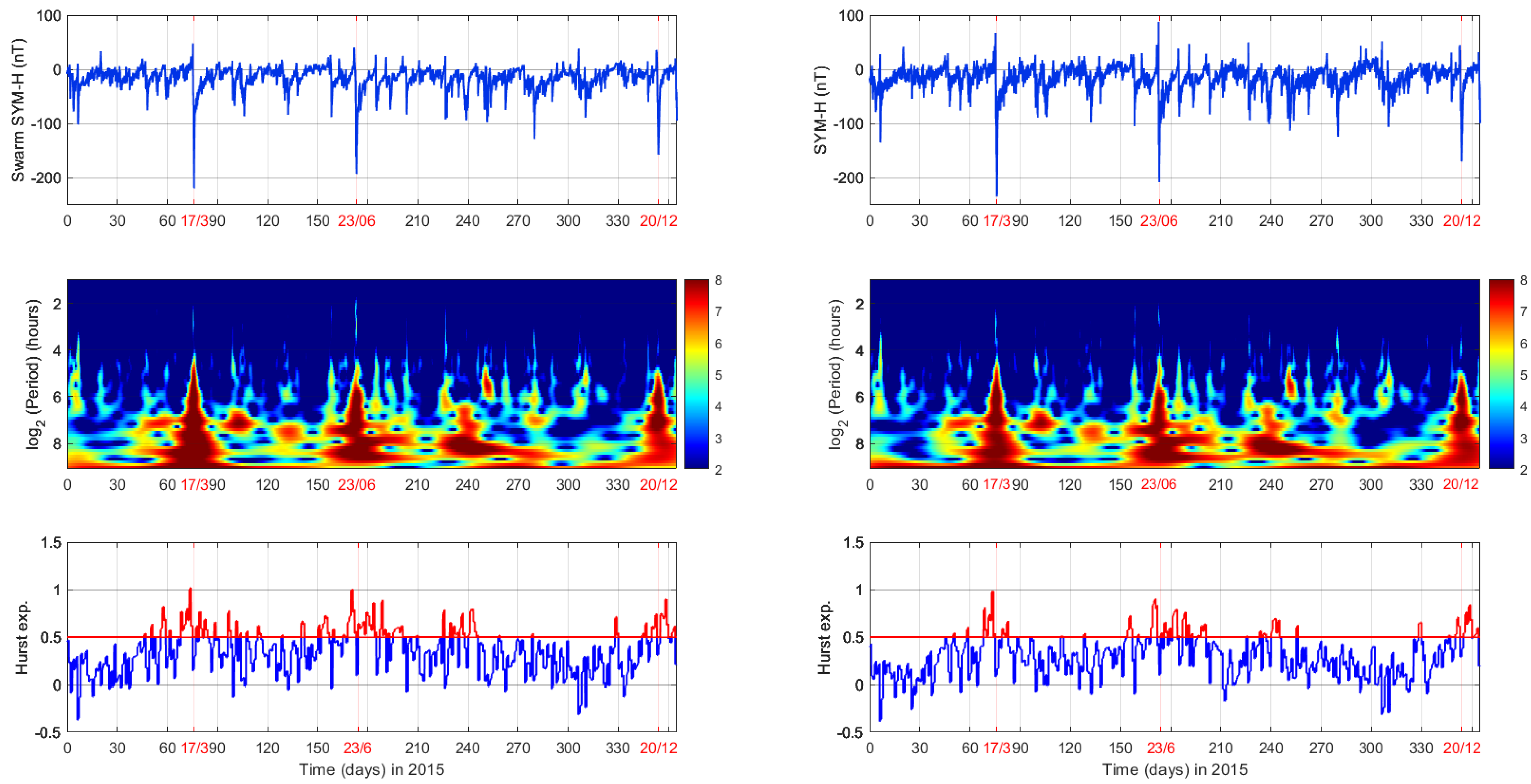
2.1. Swarm-derived SYM-H Index

The Swarm SYM-H and Swarm AE indices are derived based on a specific methodology, which is described in detail in Papadimitriou et al. [2]. For the reader’s convenience, in this section, we briefly describe the steps followed in order for the indices to be produced. Beginning with the coordinate system used for the magnetic field, the pre-processing we apply is as follows. The magnetic field measurements from the vector field magnetometer (VFM) instrument on board Swarm are provided as a three-dimensional vector in the North-East-Center coordinate system. The static, background field is removed by subtracting the internal mode of the CHAOS-7 model [36], which is comprised of the Earth’s core and crustal magnetic field contributions. The resulting measurements are then mapped to the Quasi-Dipole coordinate system [37]. From this point on, it is simple to map the vector to a mean-field-aligned coordinate system. This is achieved by projecting the total vector field onto a direction that is parallel to the model field, resulting in the creation of the Bpar component, as well as two perpendicular components, Bper1 and Bper2. Bper1 is primarily aligned with the meridional plane, pointing outwards, while Bper2 is mainly aligned along the East-West direction, pointing eastwards. For the derivation of the Swarm SYMH index, we use the Bpar component, because for the latitude region that we examine it is the component that most closely resembles that horizontal component of the terrestrial magnetic field used for constructing the ground-based SYM-H index, while for the Swarm AE index we use the total magnitude of the vector field.
The derivation of the Swarm SYM-H index is based on the following steps:
  • Extract Bpar Field Series from MAG_LR (1 Hz) product
  • Subtract CHAOS-7 [36] Internal Field Model
  • Remove obvious outliers
  • Remove values that lie above + 30 ° or below 30 ° in Magnetic Latitude
  • Apply a non-overlapping, moving average scheme on the time series, with a window of 60 s, so that the series are set to a 1-min time resolution, effectively filling up some of the smaller gaps
  • Merge Swarm A and Swarm B time series, in a joint 1-min resolution data set
  • Interpolate the remaining data gaps, using a simple linear scheme, to produce a complete time series
  • Apply a low-pass Chebyshev Type I filter with a cutoff period of 4 h, to filter out some of the small perturbations in the signal that arise from the fast motion of the satellites
  • Apply a linear transform to get the Swarm Index: S S Y M H = 1.53 B f + 12.85

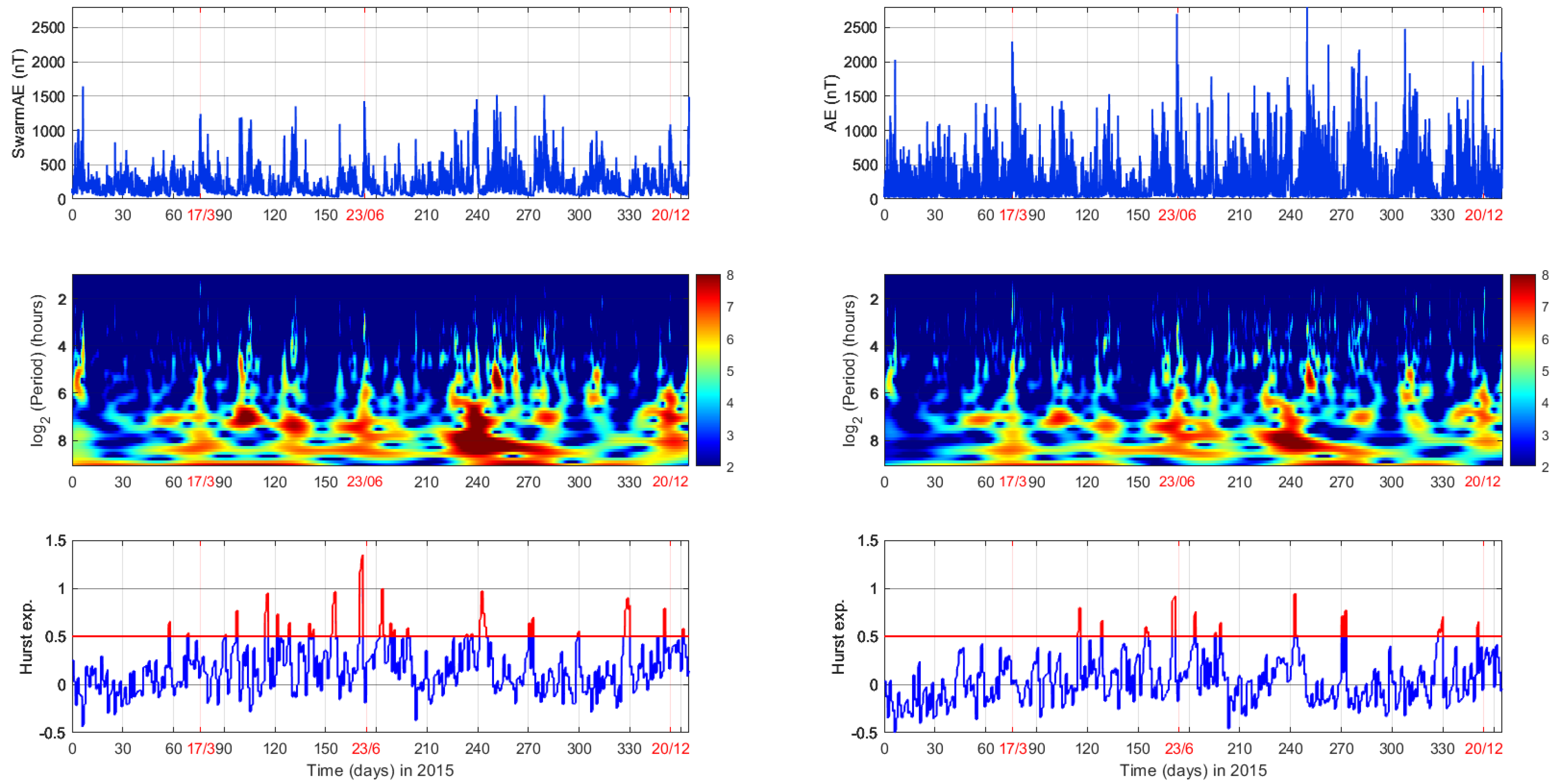
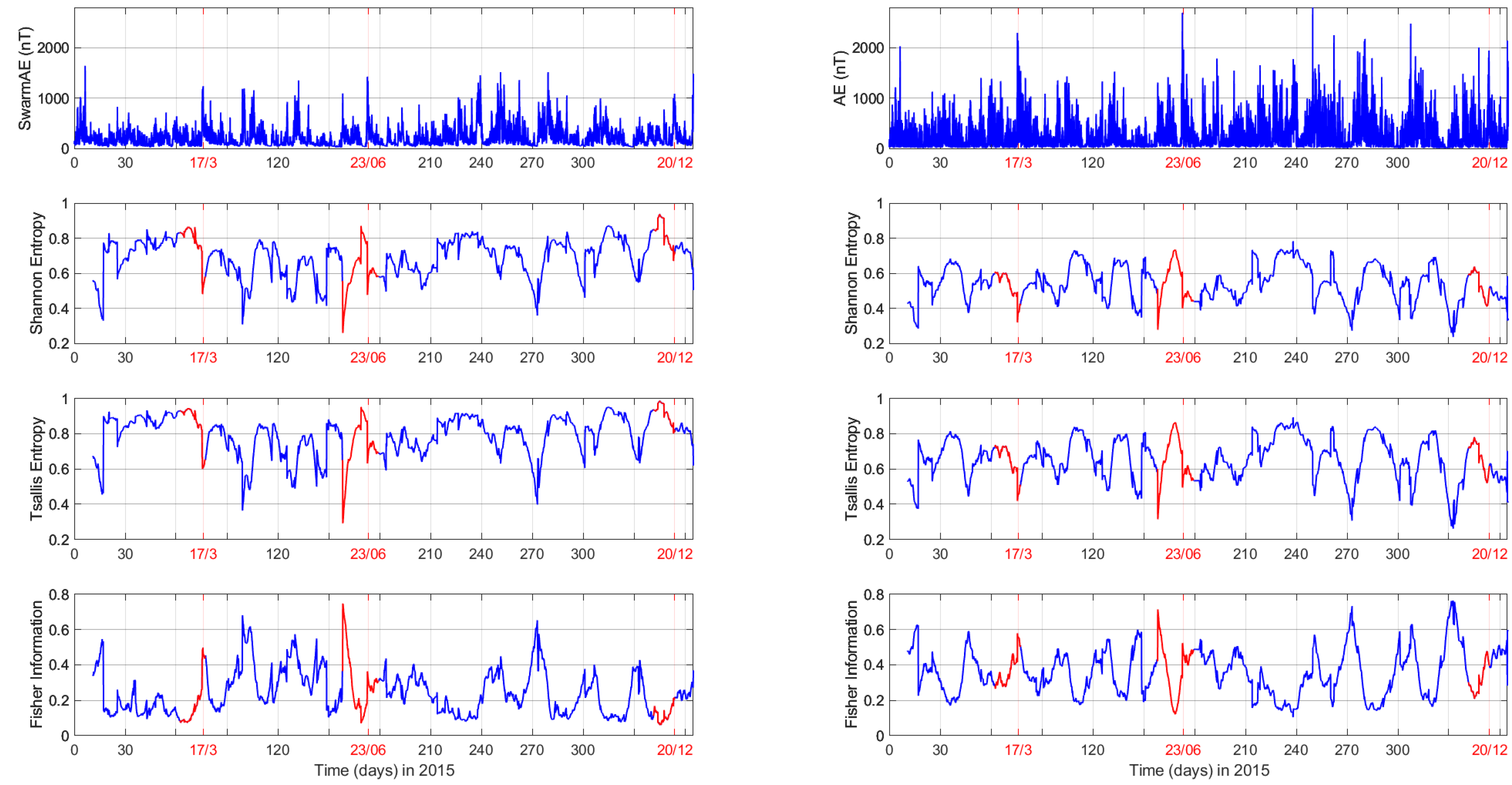
2.2. Swarm-Derived AE Index

Similarly, the Swarm AE index is derived, based on the following logic, but using simply the magnitude of the Swarm magnetic field:
  • Extract Total Magnetic Field Series from MAG_LR (1 Hz) product
  • Subtract CHAOS-7 [36] Internal Field Model
  • Remove obvious outliers
  • Keep only measurements between + 65 ° and + 75 ° (and correspondingly 75 ° to 65 ° ) in Magnetic Latitude
  • Apply a non-overlapping, moving average scheme on the time series, with a window of 60 s, so that the series are set to a 1-min time resolution, effectively filling up some of the smaller gaps
  • Merge Swarm A and Swarm B time series in a joint 1-min resolution data set
  • Interpolate the remaining data gaps, using a simple linear scheme, to produce a complete time series
  • Apply a low-pass Chebyshev Type I filter with a cutoff period of 2.6 h, to filter out some of the small perturbations in the signal that arise from the fast motion of the satellites
  • Apply a linear transform to get the Swarm Index: S A E = 2.2 B f 8.9
Various filtering thresholds and methodologies were performed to discover the optimal parameters that would yield the highest correlation scores against the corresponding ground-based SYM-H and AE indices. Applying this to the time series of the entire year 2015 produced the values of 4 h for SYM-H and 2.6 h for AE. In the final step, a linear transform was applied, with parameters that were chosen to minimize the root mean square of the difference between each Swarm index and its ground-based counterpart.

3. Overview of Methods

3.1. Hurst Exponent

If a time series is a temporal fractal, then a power law of the form S ( f ) f β is obeyed with S ( f ) the power spectral density, f the frequency and β the spectral scaling exponent, a measure of the strength of time correlations (see for instance [38,39] and references therein).
In general, 1 < β < 3 , but it describes two classes of signal [40]:
  • 1 < β < 1 : fractional Gaussian noise (fGn)
  • + 1 < β < 3 : fractional Brownian motion (fBm)
For the fBm case, β = 2 H + 1 , where H is the Hurst exponent [38,41]. The exponent H characterizes the persistent/anti-persistent properties of the signal. The range 0 < H < 0.5 ( 1 < β < 2 ) indicates anti-persistency, reflecting that if the fluctuations increase in a period, they are likely to decrease in the interval immediately following, and vice versa. The range 0.5 < H < 1 ( 2 < β < 3 ) indicates persistency, which means that if the amplitude of fluctuations increases in a time interval, it is likely to continue increasing in the interval immediately following. H = 0.5 ( β = 2 ) suggests no correlation between the repeated increments. Consequently, this particular value takes on a special physical meaning: it marks the transition between persistent and anti-persistent behavior in the time series.
The Hurst exponent provides crucial information on the kind of noise (either white or red, coming from the multifractal nature of the signal in some cases; see, for instance, Kantelhardt et al. [42], or a slightly different application in Agarwal et al. [43]).
Balasis et al. [38] analyzed the Dst index around magnetic storms in terms of the exponent H, calculated from wavelet spectra. The wavelet spectral analysis followed a power law of the form f β and showed the existence of two different patterns: (i) a pattern associated with intense magnetic storms, which can be interpreted as a fractional Brownian persistent behavior ( H > 0.5 ); (ii) a pattern associated with lower activity periods, which is interpreted as a fractional Brownian anti-persistent behavior ( H < 0.5 ). Furthermore, a series of articles [12,13,44] showed the complexity dissimilarity among “physiological” (normal) and “pathological” states (intense magnetic storms) of the magnetosphere. Entropy analysis implied the existence of two distinct patterns: (i) a pattern associated with intense magnetic storms, which is characterized by a higher degree of organization/lower complexity, and (ii) a pattern associated with lower-activity periods, which is characterized by a lower degree of organization/higher complexity.
Pitsis et al. [39] extended and verified the results of Balasis et al. [38] by applying the same wavelet analysis to the SYM-H index, the solar wind convection electric field component ( V × B s o u t h ) and several time series of the horizontal component of the Earth’s magnetic field at various locations, covering a wide range of magnetic latitudes.

3.2. Entropy Measures

In 1948, Shannon introduced a statistical concept to investigate the information size of a transmitted message [45], called information or Shannon entropy. For a discrete random variable X with a set of values Ξ , the Shannon entropy H ( X ) is defined as
H ( X ) = x Ξ p ( x ) l o g p ( x )
where p ( x ) = P r { X = x } , x Ξ is the probability distribution function of X.
Tsallis entropy can be considered a generalization of the Boltzmann–Gibbs entropy in statistical physics, and is defined as follows:
S q ( X ) = k q 1 1 x Ξ p ( x ) q
where k is Boltzmann’s constant and q is a real parameter that characterizes the degree of non-extensivity. For q→1, one can recover the Boltzmann–Gibbs entropy, which is a thermodynamic analogy of the Shannon entropy. Tsallis entropy has been widely applied in various fields of research [46]. For example, Balasis et al. have applied Tsallis entropy to quantify the dynamical complexity of magnetic storms and solar flares [47], and of time series of the disturbance storm time index [12,44].
In 1925, Fisher introduced a measure of the amount of information that can be obtained from a set of measurements [48], called Fisher information. One can write the Fisher information in its discrete form as
F = n = 1 N 1 [ p ( x n + 1 ) p ( x n ) ] 2 p ( x n )
where x n is the random variable X at time n, p ( x n ) is its probability and N is the total number of time steps. Fisher information has proved itself as a powerful method to study various nonstationary and nonlinear time series [49]. For example, it has been used to detect dynamical complexity changes associated with geomagnetic jerks [50].

4. Results

Wavelet spectral analysis is a very popular and efficient method in the study of geomagnetic field variations, as it allows for the local decomposition of nonstationary time series in either frequency or time scale and time simultaneously [51].
Herein, we apply the previously followed methodology [38,39] to compare between the Swarm SYM-H index and SYM-H index, and between the Swarm AE index and AE index. Specifically, as in Balasis et al. [38], the wavelet analysis technique using the Morlet wavelet as a basis function [52] was applied to each index’s time variations, in order to derive the coefficients of its power spectrum. Then, the power spectral densities were estimated in the frequency range from 0.5 to 60 h, using a moving window of 256 h at hourly steps of the time series, and the linear correlation coefficient r was calculated for each window to ensure that a power-law of the form S ( f ) f β is, indeed, obeyed. Finally, the spectral scaling exponent β , and thus the Hurst exponent H, is calculated for each window by performing a linear fit to the power spectral densities vs. frequency diagram (c.f. [38,39]).
Figure 1 shows the wavelet power spectra and the temporal variation of the Hurst exponent for both the Swarm SYM-H index and the SYM-H index during the year 2015, and Figure 2 shows the wavelet power spectra and the temporal variation of the Hurst exponent for both the Swarm AE index and the AE index during the year 2015.
In the wavelet power spectra (middle panels) of Figure 1, the reader is able to identify the three intense magnetic storms of 27 March, 23 June, and 20 December 2015. Intense power signal is observed around each magnetic storm’s peak, covering a wide frequency range (starting at ∼18 h and distributing all the way to the lowest periods of the spectra), thus indicating a large-scale extreme event that keeps the magnetosphere preconditioned for a long time interval (c.f. for almost a month around each of these three events). This is even more profound for the case of the Swarm SYM-H index. Regarding Figure 2, similar underlying features in the spectra can be identified for the three storms, despite the fact that we are dealing with substorm indices: the big picture of the preconditioned magnetosphere is still present. In the power spectra of all four indices (Swarm SYM-H, SYM-H, Swarm AE and AE), we also observe the existence of another area characterized by a strong spectral imprint, approximately between days 220 and 280 (mid-August to mid-October); this is the imprint of several subsequent storms (see Table 2) of smaller intensities (around −100 nT) and is better captured by the Swarm AE index. Substorm activity also seems to be well depicted by the auroral indices, with Swarm AE having a more intense power spectrum than AE throughout the whole year.
The plots of the Hurst exponent are also able to identify the disturbed periods, not only by the increase in the value of the exponent, but especially by its transition into the region of values higher than 0.5, which also marks the departure from anti-persistent behavior into the regime of persistent fractional Brownian motion. This indicates that the temporal correlations of the various increments of the signal become long-scale during these pathological states of the magnetosphere, which could also imply an increased degree of interconnectivity between the various subsystems of the terrestrial electromagnetic environment. For the SYM-H and Swarm SYM-H indices, these periods correspond with the geomagnetic storms of March, June and December, and to a slightly lesser extent, with the August–October period. For the AE indices, the image is not so clear, as the Hurst values stay almost consistently within the 0 to 0.5 range, which is characterized by anti-persistent behavior; a finding which is in agreement with the more transient and dynamic nature of substorms (in contrast to global magnetic storms).
On the one hand, from the indices themselves we cannot extract information regarding the anti-persistent vs. persistent regime accompanying either the occurrence of an intense storm (e.g., March, June, December) or the occurrence of a group of less severe storms (e.g., days 220–280). On the other hand, through the wavelet spectral and Hurst analyses of indices, for the intense events we find evidence of magnetosphere preconditioning for a time interval clearly longer than the duration of the storm (see both wavelet spectra at lower frequencies and Hurst values in Figure 1), while for the grouped weaker events the results of the same analyses imply that these storms are interrelated (again, see both wavelet spectra at lower frequencies and Hurst values in Figure 1). Furthermore, when comparing the results between satellite and ground indices in Figure 1, the same picture holds for both kinds of indices.
Figure 3 shows the Shannon and Tsallis entropy measures, as well as Fisher information, for both the Swarm SYM-H index and SYM-H index during the year 2015. Figure 4 shows the Shannon and Tsallis entropy measures, as well as Fisher information, for both the Swarm AE index and AE index during the year 2015.
There is remarkable similarity between the plots of ground-based and Swarm-derived indices, for all cases and all information measures, which indicates that the spaceborne indices have the capacity to capture the same dynamics and behaviors, with regards to their informational content, as the traditionally used ground-based ones. Especially in the case of the ring current indices (Figure 3), which are mostly associated with the three major magnetic storms of 2015, one can easily discern the shift to a state of lower entropy (i.e., high degree of organization) during these three events, indicated by the lower values of both Shannon and Tsallis entropies and the increase in Fisher information. Thus, the state of the geomagnetic system changes from a more or less random one, i.e., the random noise fluctuations of the quiet magnetosphere, to a highly organized one, as the various subsystems interact and synchronize to produce a particular phenomenon. The reader may also note in Figure 3 that, around the three intense storms, the absolute values of the three information theory measures are lower for the Swarm SYM-H index in comparison to the SYM-H index, but the general picture of the lower complexity around the time of the intense storms in comparison to the rest of the year holds for both satellite and ground indices.
This behavior, i.e., the lower complexity around the time of the three intense storms in comparison to the rest of the year, is not generally seen in the AE-related plots (Figure 4) as the auroral indices are related to substorms and not storms, so their values change in accordance with the development of the ionosphere currents in the auroral regions, phenomena which are characterized by very different time scales and occurrence frequencies. There is, however, the notable exception of the June storm, where all the information measures (Hurst exponent, entropy values and Fisher information) for the Swarm AE index attain maximum values (c.f. Figure 2 and Figure 4).

5. Discussion and Conclusions

In this study, we have analyzed 1-year-long time series from 2015 of spaceborne and ground-based geomagnetic activity indices using information theory measures, namely Hurst exponent, Shannon entropy, nonextensive Tsallis entropy and Fisher information. The LEO satellite magnetic indices were derived with data from the Swarm mission, covering the most intense magnetic storms of the previous solar cycle, including its strongest storm event, the St. Patrick’s Day storm. The analyzed indices are targeted at both storm and substorm activity.
Regarding the Swarm-derived SYM-H index and standard SYM-H index, the Hurst exponent and various entropy measures show the complexity dissimilarity among different “physiological” (normal) and “pathological” states (intense magnetic storms) of the magnetosphere. They imply the emergence of two distinct patterns: (i) a pattern associated with normal periods, which is characterized by a lower degree of organization/higher complexity, and (ii) a pattern associated with the intense magnetic storms, which is characterized by a higher degree of organization/lower complexity. These results agree well with earlier works that highlighted this transition between anti-persistent and persistent behavior around the onset of an intense storm (e.g., [12,13,25,38,41,44]).
Regarding the Swarm-derived AE index and standard AE index, the same analyses did not provide a similar picture around the storm onset in terms of the information theory measures, because these indices are concerned with substorms, which have notably different characteristic time scales and generation mechanisms than storms. In addition, substorm events occur far more often than storm events, which may contaminate the picture of the anti-persistent/persistent regime we have obtained for storm-monitoring indices. It is worth mentioning that the wavelet transform is able to capture similar spectral signatures for both the spaceborne and ground-based SYM-H and AE indices around the time of the three intense storms, which means that the global character of an extreme storm event is not depicted only in the storm-monitoring time series but also in the substorm-monitoring time variations.
The findings obtained by the application of information-theoretic approaches to the geomagnetic activity indices could be possibly exploited in subsequent work by space weather experts and space physics modellers. These findings may be utilized in order to improve forecast schemes and models of the coupled solar wind–magnetosphere–ionosphere system in terms of including information on the preconditioning of the system by the existing state of the magnetosphere [53,54].
We note that the application of the various information theory measures yields very similar results between the new Swarm-derived and standard ground-based geomagnetic activity indices. Thus, we provide evidence for the capacity of the satellite indices to capture the same dynamics and behaviors, with regards to their informational content, as the well-established ground-based indices.

Author Contributions

Conceptualization, G.B.; methodology, G.B., A.Z.B. and C.P.; software, A.Z.B., S.M.P. and V.P.; investigation, A.Z.B. and C.P.; writing—original draft preparation, G.B., A.Z.B., C.P. and S.M.P.; writing—review and editing, I.A.D., A.A. and O.G. All authors have read and agreed to the published version of the manuscript.

Funding

This study has been supported as part of Swarm DISC (Data, Innovation, and Science Cluster) activities, funded by ESA contract no. 4000109587.

Institutional Review Board Statement

Not applicable.

Informed Consent Statement

Not applicable.

Data Availability Statement

The results presented rely on the data collected by the three satellites of the Swarm constellation. Swarm data can be accessed at https://swarm-diss.eo.esa.int/, accessed on 11 March 2023.

Acknowledgments

The authors thank the European Space Agency (ESA) that supports the Swarm mission. The authors acknowledge the Kyoto World Data Center (WDC) for Geomagnetism and the observatories that produce and make SYM-H and AE indices available at http://wdc.kugi.kyoto-u.ac.jp/, accessed on 11 March 2023. The authors acknowledge support from the European Space Agency (ESA contract No. 4000125663/18/I-NB “EO Science for Society Permanently Open Call for Proposals EOEP-5 BLOCK4” [INTENS]). This research was supported by the International Space Science Institute (ISSI) in Bern, through the ISSI International Team project # 455 “Complex Systems Perspectives Pertaining to the Research of the Near-Earth Electromagnetic Environment”.

Conflicts of Interest

The authors declare no conflict of interest.

References

  1. Friis-Christensen, E.; Lühr, H.; Hulot, G. Swarm: A constellation to study the Earth’s magnetic field. Earth Planets Space 2006, 58, 351–358. [Google Scholar] [CrossRef]
  2. Papadimitriou, C.; Balasis, G.; Boutsi, A.Z.; Antonopoulou, A.; Moutsiana, G.; Daglis, I.A.; Giannakis, O.; De Michelis, P.; Consolini, G.; Gjerloev, J.; et al. Swarm-derived indices of geomagnetic activity. J. Geophys. Res. Space Phys. 2021, 126, e2021JA029394. [Google Scholar] [CrossRef]
  3. Balasis, G.; Papadimitriou, C.; Boutsi, A.Z. Ionospheric response to solar and interplanetary disturbances: A Swarm perspective. Phil. Trans. R. Soc. A 2019, 377, 20180098. [Google Scholar] [CrossRef] [PubMed]
  4. Johnson, J.R.; Wing, S. A solar cycle dependence of nonlinearity in magnetospheric activity. J. Geophys. Res. 2005, 110, A04211. [Google Scholar] [CrossRef]
  5. Wing, S.; Johnson, J.R.; Turner, D.L.; Ukhorskiy, A.Y.; Boyd, A.J. Untangling the solar wind and magnetospheric drivers of the radiation belt electrons. J. Geophys. Res. Space Phys. 2022, 127, e2021JA030246. [Google Scholar] [CrossRef]
  6. Baker, D.N.; Klimas, A.J.; McPherron, R.L.; Büchner, J. The evolution from weak to strong geomagnetic activity: An interpretation in terms of deterministic chaos. Geophys. Res. Lett. 1990, 17, 41–44. [Google Scholar] [CrossRef]
  7. Tsurutani, B.T.; Sugiura, M.; Iyemori, T.; Goldstein, B.E.; Gonzalez, W.D.; Akasofu, S.-I.; Smith, E.J. The nonlinear response of AE to the IMF BS driver: A spectral break at 5 hours. Geophys. Res. Lett. 1990, 17, 279–282. [Google Scholar] [CrossRef]
  8. Vassiliadis, D.V.; Sharma, A.S.; Eastman, T.E.; Papadopoulos, K. Low-dimensional chaos in magnetospheric activity from AE time series. Geophys. Res. Lett. 1990, 17, 1841–1844. [Google Scholar] [CrossRef]
  9. Sharma, A.S.; Vassiliadis, D.V.; Papadopoulos, K. Reconstruction of low-dimensional magnetospheric dynamics by singular spectrum analysis. Geophys. Res. Lett. 1993, 20, 335. [Google Scholar] [CrossRef]
  10. Sitnov, M.I.; Sharma, A.S.; Papadopoulos, K.; Vassiliadis, D. Modeling substorm dynamics of the magnetosphere: From self-organization and self-organized criticality to nonequilibrium phase transitions. Phys. Rev. E 2001, 65, 16116. [Google Scholar] [CrossRef]
  11. Consolini, G.; De Michelis, P.; Tozzi, R. On the Earth’s magnetospheric dynamics: Nonequilibrium evolution and the fluctuation theorem. J. Geophys. Res. Space Phys. 2008, 113, A08222. [Google Scholar] [CrossRef]
  12. Balasis, G.; Daglis, I.A.; Papadimitriou, C.; Kalimeri, M.; Anastasiadis, A.; Eftaxias, K. Investigating dynamical complexity in the magnetosphere using various entropy measures. J. Geophys. Res. Space Phys. 2009, 114, A00D06. [Google Scholar] [CrossRef]
  13. Balasis, G.; Donner, R.V.; Potirakis, S.M.; Runge, J.; Papadimitriou, C.; Daglis, I.A.; Eftaxias, K.; Kurths, J. Statistical mechanics and information-theoretic perspectives on complexity in the earth system. Entropy 2013, 15, 4844–4888. [Google Scholar] [CrossRef]
  14. Wing, S.; Johnson, J.R.; Camporeale, E.; Reeves, G.D. Information theoretical approach to discovering solar wind drivers of the outer radiation belt. J. Geophys. Res. Space Phys. 2016, 121, 9378–9399. [Google Scholar] [CrossRef]
  15. Donner, R.V.; Stolbova, V.; Balasis, G.; Donges, J.F.; Georgiou, M.; Potirakis, S.M.; Kurths, J. Temporal organization of magnetospheric fluctuations unveiled by recurrence patterns in the Dst index. Chaos 2018, 28, 085716. [Google Scholar] [CrossRef]
  16. Donner, R.V.; Balasis, G.; Stolbova, V.; Georgiou, M.; Wiedermann, M.; Kurths, J. Recurrence based quantification of dynamical complexity in the Earth’s magnetosphere at geospace storm timescales. J. Geophys. Res. Space Phys. 2019, 124, 90–108. [Google Scholar] [CrossRef]
  17. Johnson, J.R.; Wing, S.; Camporeale, E. Transfer entropy and cumulant-based cost as measures of nonlinear causal relationships in space plasmas: Applications to Dst. Ann. Geophys. 2018, 36, 945–952. [Google Scholar] [CrossRef]
  18. Runge, J.; Balasis, G.; Daglis, I.A.; Papadimitriou, C.; Donner, R.V. Common solar wind drivers behind magnetic storm–magnetospheric substorm dependency. Sci. Rep. 2018, 8, 1–10. [Google Scholar] [CrossRef]
  19. Stumpo, M.; Consolini, G.; Alberti, T.; Quattrociocchi, V. Measuring Information Coupling between the Solar Wind and the Magnetosphere–Ionosphere System. Entropy 2020, 22, 276. [Google Scholar] [CrossRef]
  20. Manshour, P.; Balasis, G.; Consolini, G.; Papadimitriou, C.; Paluš, M. Causality and Information Transfer Between the Solar Wind and the Magnetosphere–Ionosphere System. Entropy 2021, 23, 390. [Google Scholar] [CrossRef]
  21. Osmane, A.; Savola, M.; Kilpua, E.; Koskinen, H.; Borovsky, J.E.; Kalliokoski, M. Quantifying the non-linear dependence of energetic electron fluxes in the Earth’s radiation belts with radial diffusion drivers. Ann. Geophys. 2022, 40, 37–53. [Google Scholar] [CrossRef]
  22. Balasis, G.; Papadimitriou, C.; Boutsi, A.Z.; Daglis, I.A.; Giannakis, O.; Anastasiadis, A.; De Michelis, P.; Consolini, G. Dynamical complexity in Swarm electron density time series using Block entropy. Europhys. Lett. 2020, 131, 69001. [Google Scholar] [CrossRef]
  23. De Michelis, P.; Pignalberi, A.; Consolini, G.; Coco, I.; Tozzi, R.; Pezzopane, M.; Giannattasio, F.; Balasis, G. On the 2015 St. Patrick’s Storm Turbulent State of the Ionosphere: Hints From the Swarm Mission. J. Geophys. Res. Space Phys. 2020, 125, e2020JA027934. [Google Scholar] [CrossRef]
  24. De Michelis, P.; Consolini, G.; Pignalberi, A.; Tozzi, R.; Coco, I.; Giannattasio, F.; Pezzopane, M.; Balasis, G. Looking for a proxy of the ionospheric turbulence with Swarm data. Sci. Rep. 2021, 11, 6183. [Google Scholar] [CrossRef]
  25. Papadimitriou, C.; Balasis, G.; Boutsi, A.Z.; Daglis, I.A.; Giannakis, O.; Anastasiadis, A.; De Michelis, P.; Consolini, G. Dynamical Complexity of the 2015 St. Patrick’s Day Magnetic Storm at Swarm Altitudes Using Entropy Measures. Entropy 2020, 22, 574. [Google Scholar] [CrossRef]
  26. Consolini, G.; Tozzi, R.; De Michelis, P.; Coco, I.; Giannattasio, F.; Pezzopane, F.; Marcucci, M.F.; Balasis, G. High-latitude polar pattern of ionospheric electron density: Scaling features and IMF dependence. J. Atmos.-Sol.-Terr. Phys. 2021, 217, 105531. [Google Scholar] [CrossRef]
  27. Poduval, B.; Pitman, K.M.; Verkhoglyadova, O.; Wintoft, P. Editorial: Applications of statistical methods and machine learning in the space sciences. Front. Astron. Space Sci. 2023, 10, 5–9. [Google Scholar] [CrossRef]
  28. Delzanno, G.L.; Borovsky, J.E. The Need for a System Science Approach to Global Magnetospheric Models. Front. Astron. Space Sci. 2022, 9, 10–16. [Google Scholar] [CrossRef]
  29. Telloni, D. Statistical Methods Applied to Space Weather Science. Front. Astron. Space Sci. 2022, 9, 154–160. [Google Scholar] [CrossRef]
  30. Verkhoglyadova, O.; Meng, X.; Kosberg, J. Understanding Large-Scale Structure in Global Ionospheric Maps with Visual and Statistical Analyses. Front. Astron. Space Sci. 2022, 9, 78–81. [Google Scholar] [CrossRef]
  31. Dungey, J.W. Interplanetary magnetic field and the auroral zones. Phys. Rev. Lett. 1961, 6, 47–48. [Google Scholar] [CrossRef]
  32. Bergin, A.; Chapman, S.; Gjerloev, J. AE, Dst and their SuperMAG Counterparts: The effect of improved spatial resolution in geomagnetic indices. J. Geophys. Res. Space Phys. 2020, 125, e2020JA027828. [Google Scholar] [CrossRef]
  33. Balasis, G.; Daglis, I.A.; Contoyiannis, Y.; Potirakis, S.M.; Papadimitriou, C.; Melis, N.S.; GIannakis, O.; Papaioannou, A.; Anastasiadis, A.; Kontoes, C. Observation of intermittency-induced critical dynamics in geomagnetic field time series prior to the intense magnetic storms of March, June, and December 2015. J. Geophys. Res. Space Phys. 2018, 123, 4594–4613. [Google Scholar] [CrossRef]
  34. Tozzi, R.; De Michelis, P.; Coco, I.; Giannattasio, F. A preliminary risk assessment of geomagnetically induced currents over the Italian territory. Space Weather 2019, 17, 46–58. [Google Scholar] [CrossRef]
  35. Boutsi, A.Z.; Balasis, G.; Dimitrakoudis, S.; Daglis, I.A.; Tsinganos, K.; Papadimitriou, C.; Giannakis, O. Investigation of the geomagnetically induced current index levels in the Mediterranean region during the strongest magnetic storms of solar cycle 24. Space Weather 2023, 21, e2022SW003122. [Google Scholar] [CrossRef]
  36. Finlay, C.C.; Kloss, C.; Olsen, N.; Hammer, M.; Toeffner-Clausen, L.; Grayver, A.; Kuvshinov, A. The CHAOS-7 geomagnetic field model and observed changes in the South Atlantic Anomaly. Earth Planets Space 2020, 72, 156. [Google Scholar] [CrossRef]
  37. Emmert, J.T.; Richmond, A.D.; Drob, D.P. A computationally compact representation of Magnetic-Apex and Quasi-Dipole coordinates with smooth base vectors. J. Geophys. Res. 2010, 115, A08322. [Google Scholar] [CrossRef]
  38. Balasis, G.; Daglis, I.; Kapiris, P.; Mandea, M.; Vassiliadis, D.; Eftaxias, K. From pre-storm activity to magnetic storms: A transition described in terms of fractal dynamics. Ann. Geophys. 2006, 24, 3557–3567. [Google Scholar] [CrossRef]
  39. Pitsis, V.; Balasis, G.; Daglis, I.A.; Vassiliadis, D.; Boutsi, A.Z. Power-law dependence of the wavelet spectrum of ground magnetic variations during magnetic storms. Adv. Space Res. 2023, 71, 2288–2298. [Google Scholar] [CrossRef]
  40. Heneghan, C.; McDarby, G. Establishing the relation between detrended fluctuation analysis and power spectral density analysis for stochastic processes. Phys. Rev. E. 2000, 62, 6103–6110. [Google Scholar] [CrossRef]
  41. Alberti, T.; Consolini, G.; De Michelis, P. Complexity of geomagnetic index in the last two solar cycles. J. Atmos. Solar Terr. Phys. 2021, 217, 105583. [Google Scholar] [CrossRef]
  42. Kantelhardt, J.W.; Zschiegner, S.A.; Koscielny-Bunde, E.; Havlin, S.; Bunde, A.; Stanley, H.E. Multifractal detrended fluctuation analysis of nonstationary time series. Phys. A Stat. Mech. Its Appl. 2002, 316, 87–114. [Google Scholar] [CrossRef]
  43. Agarwal, S.; Del Sordo, F.; Wettlaufer, J.S. Exoplanetary detection by multifractal spectral analysis. Astron. J. 2017, 153, 12. [Google Scholar] [CrossRef]
  44. Balasis, G.; Daglis, I.A.; Papadimitriou, C.; Kalimeri, M.; Anastasiadis, A.; Eftaxias, K. Dynamical complexity in Dst time series using non-extensive Tsallis entropy. Geophys. Res. Lett. 2008, 35, L14102. [Google Scholar] [CrossRef]
  45. Shannon, C.E. A mathematical theory of communication. Bell Syst. Tech. J. 1948, 27, 379–423. [Google Scholar] [CrossRef]
  46. Tsallis, C. Introduction to Nonextensive Statistical Mechanics: Approaching a Complex World; Springer: New York, NY, USA, 2009; Volume 1. [Google Scholar]
  47. Balasis, G.; Daglis, I.A.; Papadimitriou, C.; Anastasiadis, A.; Sandberg, I.; Eftaxias, K. Quantifying dynamical complexity of magnetic storms and solar flares via nonextensive Tsallis entropy. Entropy 2011, 13, 1865–1881. [Google Scholar] [CrossRef]
  48. Fisher, R.A. Theory of statistical estimation. In Mathematical Proceedings of the Cambridge Philosophical Society; Cambridge University Press: Cambridge, UK, 1925; Volume 22, pp. 700–725. [Google Scholar]
  49. Martin, M.T.; Pennini, F.; Plastino, A. Fisher’s information and the analysis of complex signals. Phys. Lett. A 1999, 256, 173–180. [Google Scholar] [CrossRef]
  50. Balasis, G.; Potirakis, S.M.; Mandea, M. Investigating dynamical complexity of geomagnetic jerks using various entropy measures. Front. Earth Sci. 2016, 4, 71. [Google Scholar] [CrossRef]
  51. Katsavrias, C.; Papadimitriou, C.; Hillaris, A.; Balasis, G. Application of Wavelet Methods in the Investigation of Geospace Disturbances: A Review and an Evaluation of the Approach for Quantifying Wavelet Power. Atmosphere 2022, 13, 499. [Google Scholar] [CrossRef]
  52. Torrence, G.; Compo, P. A practical guide to wavelet analysis. Am. Meteorol. Soc. 1998, 79, 61–78. [Google Scholar] [CrossRef]
  53. Borovsky, J.E. Is Our Understanding of Solar-Wind/Magnetosphere Coupling Satisfactory? Front. Astron. Space Sci. 2021, 8, 634073. [Google Scholar] [CrossRef]
  54. Lockwood, M. The Joined-Up Magnetosphere. Front. Astron. Space Sci. 2022, 9, 856188. [Google Scholar] [CrossRef]
Figure 1. Swarm SYM-H index (left column) and SYM-H index (right column): time series (top row), wavelet spectra analysis (middle row) and Hurst exponent (bottom row) for the year 2015. The red line at 0.5 marks the transition from the anti-persistent behavior (blue) into the persistent fractional Brownian motion (red).
Atmosphere 14 00890 g001
Figure 2. Swarm AE index (left column) and AE index (right column): time series (top row), wavelet spectra analysis (middle row) and Hurst exponent (bottom row) for the year 2015. The red line at 0.5 marks the transition from the anti-persistent behavior (blue) into the persistent fractional Brownian motion (red).
Atmosphere 14 00890 g002
Figure 3. SYM-H index (left column) and SYM-H index (right column): time series (top row), Shannon entropy, Tsallis entropy and Fisher information (bottom row) for the year 2015. Red color is used to highlight the entropy values around the three magnetic storms of 2015 (17/3, 23/6 and 20/12).
Atmosphere 14 00890 g003
Figure 4. Swarm AE index (left column) and AE index (right column): time series (top row), Shannon entropy, Tsallis entropy and Fisher information (bottom row) for the year 2015. Red color is used to highlight the entropy values around the three magnetic storms of 2015 (17/3, 23/6 and 20/12).
Atmosphere 14 00890 g004
Table 1. Intense geospace magnetic storms of 2015, including the St. Patrick’s Day storm, which was the strongest storm of solar cycle 24 (2008–2019). Storm date, time and minimum Dst index value reached are given in the second, third and fourth columns, respectively.
CaseStorm DateStorm Time (UT)Dst (nT)
#117 March 201522:00:00−223
#223 June 201504:00:00−204
#320 December 201522:00:00−155
Table 2. Geospace magnetic storms between mid-August and mid-October 2015. Storm date, time and minimum Dst index value reached are given in the first, second and third columns, respectively.
Storm DateStorm Time (UT)Dst (nT)
16 August 201508:00:00−98
26 August 201522:00:00−79
27 August 201521:00:00−103
28 August 201510:00:00−102
09 September 201513:00:00−105
11 September 201515:00:00−87
20 September 201516:00:00−81
07 October 201523:00:00−130
Disclaimer/Publisher’s Note: The statements, opinions and data contained in all publications are solely those of the individual author(s) and contributor(s) and not of MDPI and/or the editor(s). MDPI and/or the editor(s) disclaim responsibility for any injury to people or property resulting from any ideas, methods, instructions or products referred to in the content.

