N₂O Temporal Variability from the Middle Troposphere to the Middle Stratosphere Based on Airborne and Balloon-Borne Observations during the Period 1987–2018

Abstract

Nitrous oxide (N₂O) is the fourth most important greenhouse gas in the atmosphere and is considered the most important current source gas emission for global stratospheric ozone depletion (O₃). It has natural and anthropogenic sources, mainly as an unintended by-product of food production activities. This work examines the identification and quantification of trends in the N₂O concentration from the middle troposphere to the middle stratosphere (MTMS) by in situ and remote sensing observations. The temporal variability of N₂O is addressed using a comprehensive dataset of in situ and remote sensing N₂O concentrations based on aircraft and balloon measurements in the MTMS from 1987 to 2018. We determine N₂O trends in the MTMS, based on observations. This consistent dataset was also used to study the N₂O seasonal cycle to investigate the relationship between abundances and its emission sources through zonal means. The results show a long-term increase in global N₂O concentration in the MTMS with an average of 0.89 ± 0.07 ppb/yr in the troposphere and 0.96 ± 0.15 ppb/yr in the stratosphere, consistent with 0.80 ppb/yr derived from ground-based measurements and 0.799 ± 0.024 ppb/yr ACE-FTS (Atmospheric Chemistry Experiment Fourier Transform Spectrometer) satellite measurements.

1. Introduction

Nitrous oxide (N₂O) plays a critical role in Earth’s atmosphere. In the troposphere, it absorbs infrared radiation and thus contributes to global warming. Because of this absorption capacity and its long lifetime of 118 ± 7 years (average value derived from [1,2]), N₂O is the fourth most important greenhouse gas in the atmosphere [3]. Natural N₂O emissions mainly come from bacterial nitrification and de-nitrification reactions in soils and the oceans. The primary anthropogenic sources are the use of nitrogen fertilizers in agriculture for food production, with minor contributions from the combustion of biomass and biofuels, traffic, and some industrial activities such as chemical production [4]. The primary atmospheric sink for N₂O is photolysis in the stratosphere, which produces N₂ and O. However, a small fraction of N₂O is destroyed by reaction with excited oxygen atoms (O(¹D)). The latter reaction has two pathways, one being the primary pathway to generate NO in the stratosphere. NO can then play many important roles in the stratosphere. Of particular importance is its ability to catalytically destroy stratospheric ozone (O₃) in the cycle involving nitrogen oxides (NO_x = NO + NO₂) ([5] and references therein). Ravishankara et al. [6] showed that anthropogenic N₂O emissions are currently the largest contributor to ozone-depleting substances’ emissions.

N₂O is well mixed in the troposphere due to its stability and long residence time. It is transported into the stratosphere primarily through the tropics (Brewer–Dobson circulation) and shows a general decrease in concentration with altitude in the stratosphere due to the reactions cited above. The Brewer–Dobson circulation generates a latitudinal gradient; N₂O stratospheric concentrations peak near the equator and decrease towards the poles. A difference in tropospheric concentration is also observed between the two hemispheres, where the Northern Hemisphere, with its larger terrestrial surface and population, is the primary source of N₂O emissions [7].

Since 1970, the tropospheric N₂O concentration measured at the surface has increased at a roughly constant growth rate [8]. It is expected to continue rising in line with increasing human population, as emissions are tied mainly to food production. Global mean N₂O volume mixing ratios rose by 0.8 ppb yr⁻¹ [9], resulting in the annual surface global mean N₂O mole fraction reaching 336 ppb [9], compared to its pre-industrial value of 271 ppb [4,9]. In 2016, N₂O contributed 0.19 W m⁻² to global radiative forcing, approximately 10% of that for CO₂ [9]. As emissions of ozone-depleting substances (ODS) diminish in accordance with the Montreal Protocol and subsequent amendments, N₂O, together with CH₄ and CO₂, will become the main drivers of global stratospheric O₃ change in the second half of the 21st century.

Ground-based measurements have limited spatial coverage and do not cover the globe equally. In situ measurements from aircraft and balloon campaigns cover a broader area, with a dense observation network, in particular, due to the deployment of measurements onboard commercial aircraft. These observations lead to a more global picture of trace gas distribution with less potential bias due to restricted or preferred measurement areas. Furthermore, this has the advantage of providing direct in situ measurements over the vertical column, with no model based a priori, in contrast to column measurements from space or the ground. Direct in situ measurements also offer the advantage of providing a reliable approach to monitoring the temporal trend in N₂O concentration, as the continuous improvement in measurement techniques gives access to accurate measurements. However, the improvement in techniques (or changes in techniques over time) can also introduce bias in the detection of trends. This bias is minimized by using similar N₂O standards for various techniques. The statistical methods described here can also reduce errors.

In this paper, we assemble N₂O aircraft and balloon measurements from research campaigns covering 1987–2018 for altitudes ranging up to the mid-stratosphere. Our objective is to use these observations to evaluate the N₂O trend from the middle troposphere to the middle stratosphere (MTMS), and compare it with the trend obtained with surface and satellite observations.

This paper is structured as follows. Section 2 describes the different datasets (aircraft, balloon) and the use of statistical analysis to provide quality control on the data. Section 3 presents and discusses the results for the temporal variability and the seasonal zonal mean values of N₂O derived from aircraft/balloon measurements. We end with Section 4, which summarizes the results and puts the historical observed abundance in perspective with future projections.

2. Data Description and Methods

2.1. Aircraft and Balloon Observations

The data we have compiled here represent the most extensive dataset among those available from research aircraft and balloon campaigns; they are listed in Appendix A. Almost 2.5 million measurements from 53 research campaigns have been collected from 1987 until 2018 at pressure levels ranging from 600 to 5 hPa. This unique dataset includes measurements from stratospheric balloon flights, the Space Shuttles, instrumented commercial aircraft, and several research aircraft campaigns. The research aircraft campaigns include measurements using the ER-2, Global Hawk and DC8 (managed by NASA Armstrong (Dryden) Flight Research Center, USA), WB57 (managed by NASA Johnson Space Center, USA), the Learjet (managed by Enviscope GFD, Germany) and HALO and Falcon (managed by DLR, Germany), the NSF/NCAR HIAPER Gulfstream GV (Broomfield, Colorado, USA, managed by EOL’s Research Aviation Facility), and the Geophysica M55 (produced by Myasishchev Design Bureau, Zhukovsky, Russia). The measurements were performed using three kinds of instruments: (1) optical instruments (in situ spectrometers, remote sensing spectrometers, and radiometers), (2) online instruments, and (3) offline chromatographic techniques (using NOAA standard scale), listed in

Table 1. Instruments list and characteristics.

Instrument	Contact Person	References
Optical Techniques
ALIAS	C. R. Webster	[10]
ALIAS-II AL	L. Christensen	[10]
ARGUS N2	M. Loewenstein	[11]
ASUR	H. Küllmann, A. Kleinböhl	[12]
ATLAS	M. Loewenstein	[13]
ATLAS N2	James Podolske	[13]
ATMOS	M. R. Gunson	[14]
DACOM	G. S. Diskin	[15]
FIRS-2	K. Jucks	[16]
MIPAS-B	F. Friedl-Vallon, G. Wetzel	[17]
MkIV	G. C. Toon, A. Kleinböhl	[18]
QCLS	S. Wofsy	[19,20,21,22]
SLS	R. A. Stachnik	[23]
SPIRALE	V. Catoire	[24,25]
TRIHOP	P. Hoor	[26,27,28]
TRISTAR	P. Hoor	[29]
COLD2	S. Viciani, F. Damato	[30,31]
UMAQS	P. Hoor	[32,33]
Chromatographic techniques
ACATS	J. W. Elkins, D. Hurst	[34,35]
UCATS	D. Hurst, E. Hintsa	[36]
LACE	J. W. Elkins, F. Moore	[37]
PANTHER	J. W. Elkins, F. Moore	[38]
UC Irvine WAS	D. R. Blake	[39]
WAS	E. Atlas	[40,41]
PFP	S. Montzka	[42,43]
BONBON	A. Engel	[44]
TRAC and HIRES	T. Schuck, J. Williams	[45]

(more information about campaigns is given in Appendix A). Figure 1 illustrates the spatial and seasonal coverage of all the gathered data. The global coverage shows that all the continents are represented; however, some have fewer observations than others. Overall, the measurements cover broad altitude and latitude ranges, with pressure levels reaching values as low as about 5 hPa (~35 km), mainly in the Northern Hemisphere. A greater coverage for all latitudes and seasons down to 40 hPa is seen in Figure 1b. We use the observations between 600 hPa (free troposphere, ~4 km) and 5 hPa (mid-stratosphere) for this study. In winter and summer, the coverage of the latitudes between 0° and 90° S for pressures lower than 40 hPa is sparse compared to the other seasons. The observations mainly cover North America, a large part of Europe, New Zealand, and the southern part of South America, and are densest in the Northern Hemisphere.

2.2. Quality Control and Representativity of the Data

One of the major issues with inhomogeneous data is the inevitable presence of outliers. Outlier identification requires the ability to compare observations collected under similar conditions (same latitude and pressure). Such identification is routinely done by binning the data according to latitude and pressure (first finding a suitable compromise between bin size and the number of observations in each bin) and then detecting outliers in each bin. This approach is challenged here by the sparsity of the observations. To overcome this problem, we developed a different approach that avoids binning by using the high reproducibility of the concentration profiles.

As a first check, we take advantage of the expected monotonic vertical profiles and use only the measurements made over a given location. For example, for in situ measurements, we only use observations made during the ascent or descent phase of the balloon/aircraft, and not those collected during altitude plateaus. Latitude changes during plateaus can sometimes be important, however, as they might potentially modify the N₂O concentration at the same altitude. Some flights had to be split into several profiles.

Next, we exploit the reproducibility of the profiles. Figure 2 illustrates N₂O concentration profiles versus pressure and shows that they all have a similar shape, although with greater relative dispersion in the stratosphere. This reproducibility of the concentration profiles suggests that each can be expressed by the same shape (regardless of its amplitude) with minor changes. One can then considerably simplify the analysis by describing these profiles as a combination of characteristic shapes, hereafter called modes.

In Appendix B, we show that the salient features of all profiles can be adequately described by a linear combination of only two modes. That is, the observed concentration profile $c_k\left(p\right)$ of the k′th observation at pressure p can be approximated by the model ${\widehat{c}}_k\left(p\right)$:

$${\widehat{c}}_k\left(p\right)=A_{1,k}{m}_1\left(p\right)+A_{2,k}{m}_2\left(p\right)$$

(1)

where $m_1\left(p\right)$ and $m_2\left(p\right)$ are the two modes, and $A_{1,k}$ and $A_{2,k}$ are their respective amplitudes. The two modes can be interpreted as representative profiles such that the observed concentration is a latitude-dependent linear combination of them. The presence of two modes implies the existence of only two degrees of freedom in the observed profile shapes. This number of degrees results from a trade-off between the data quality and the observed shapes’ diversity. Its low value is a consequence of the similarity of all the shapes displayed in Figure 2.

The two modes are displayed in Figure 2. Their amplitudes are arbitrary because they are scaled by $A_{i,k}$. We estimate both by blind source separation [46], which is closely related to the simpler and better-known empirical orthogonal functions [47].

Let us stress that the modes are statistical and therefore have no immediate physical meaning. Nevertheless, mode 1 can readily be associated with a typical profile, whereas mode 2 expresses the correction to describe regimes with enhanced N₂O concentrations in the stratosphere.

Figure 3 shows the amplitude of both modes versus latitude and reveals a clear latitudinal dependence, with increasing scatter at high latitudes. As expected, mode 1 is dominant. However, mode 2, which captures regimes with relatively higher stratospheric N₂O concentrations, increases rapidly at high latitudes. The sum of the two amplitudes is approximately constant because all concentrations must eventually reach the same value in the lower troposphere.

Finally, we compare the observed concentration profile $c_k\left(p\right)$ with the model ${\widehat{c}}_k\left(p\right)$ from Equation (1) to locate outliers for each profile. We compute their difference and use the sum of squares as a global measure of discrepancy:

$$J_k={\sum _p\left(c_k\left(p\right)-{\widehat{c}}_k\left(p\right)\right)}^2$$

(2)

We normalize the value of J_k to the number of observations to facilitate the comparison of profiles with different vertical extents. Hence, larger the J_k, more the k′th profile differs from the family of observed profiles. For each pressure, the distribution of J reveals a core of relatively small values with an exponential tail of large errors. In the following, we set the cutoff at 90th percentiles to retain the smallest values only. In doing so, we discard those observations whose profiles belong to the largest 10% of values of J. A visual inspection of these profiles confirms that they indeed show suspicious variations with pressure and/or contain anomalous peaks.

This pre-processing allows us to create a matrix of “typical” profiles binned according to pressure (between 600 and 5 hPa) for 1820 profiles. Next, for each large latitude band defining the high latitudes or polar (±[90–60]° N), midlatitudes (±[60–30]° N), and tropics (±30° N), we create a profile and extract a standard deviation. Therefore, we create five profiles that allow us to sort the data set in terms of outliers and exclude particular dynamic cases such as tropical intrusions.

Following this, we process all measurements and classify them according to the five latitude bands. All data that are not within ±3 σ of the average profiles are excluded; they represent 2.6% of the total. These data are not only outliers but potentially also special dynamic cases such as tropical or tropospheric intrusions, stratospheric descents, etc., which would lead to biases in calculating the means. In total, 2,435,700 N₂O measurements are extracted that way (97.4% of the original total) for all latitudes and pressures between 600 and 5 hPa.

Figure 4 shows the number of measurements (points) in 10° latitude bins, 60 pressure levels, and for the four seasons: DJF (December, January, February), MAM (March, April, May), JJA (June, July, August), and SON (September, October, November). The plot shows good coverage of the Northern Hemisphere with more than 200 measurements per box for the four seasons. The lower stratosphere is well represented with over 1000 points per box for all latitudes. The middle stratosphere (c.a. 50–5 hPa) in the Southern Hemisphere is poorly or not at all observed for some boxes (as compared to the Northern Hemisphere).

2.3. Data Handling

From the curated dataset, we create a 3D grid of latitudes, pressures, and time with latitudes for South and North Polar areas (±[90–60]° N), northern and southern midlatitudes (±[60–30]° N) and tropics (±30°), and with 24 pressure levels (from 600 hPa to 5 hPa) and seasons of each year (1987–2018), i.e., 5 latitudes boxes × 23 pressure boxes × 4 seasons × 32 years as 14,720 “boxes.” To take into account that some measurements are more precise than others in the same box, the instrumental error-weighted average is calculated following this equation:

$$\widehat{\mu }=\sum _{i=1}^n{x}_i\times w_i$$

(3)

where n is the number of measurements in one box, $w_i\propto 1/{err}_i^2$ is the normalized weight with ${\sum }_{i=1}^n{w}_i=1$, and x_i is the N₂O concentration for the measurement i associated with the instrumental error err_i.

For each box, the standard deviation of the weighted average is calculated:

$$\widehat{\sigma }=\sqrt{\sum _{i=0}^n{w}_i\times {\left(x_i-\widehat{\mu }\right)}^2}$$

(4)

These calculations allow us to extract the slope of the concentration versus time (Section 3.1) and the trend in ppb/yr for each latitude band and pressure level.

Additional insight can be gained by taking the N₂O zonal mean over all the years. Boxes of latitude and pressure are created with latitude bins every 10°, and with 60 pressure levels (from 600 hPa to 5 hPa) and four seasons (i.e., 18 latitude boxes × 59 pressure boxes × 4 seasons as 4248 “boxes”). Equations (3) and (4) are applied for each box with x_i recalculated to the concentration of 2018 by applying a factor corresponding to the trend extracted in Section 3.1 as follows:

$$x_i\left(2018\right)=x_i\left(t\right)+trend (ppb/yr)\times (2018-t)$$

(5)

where t is the time (in years) of the measurement. From these boxes, we estimate and discuss zonal means in Section 3.2.

3. Results and Discussion

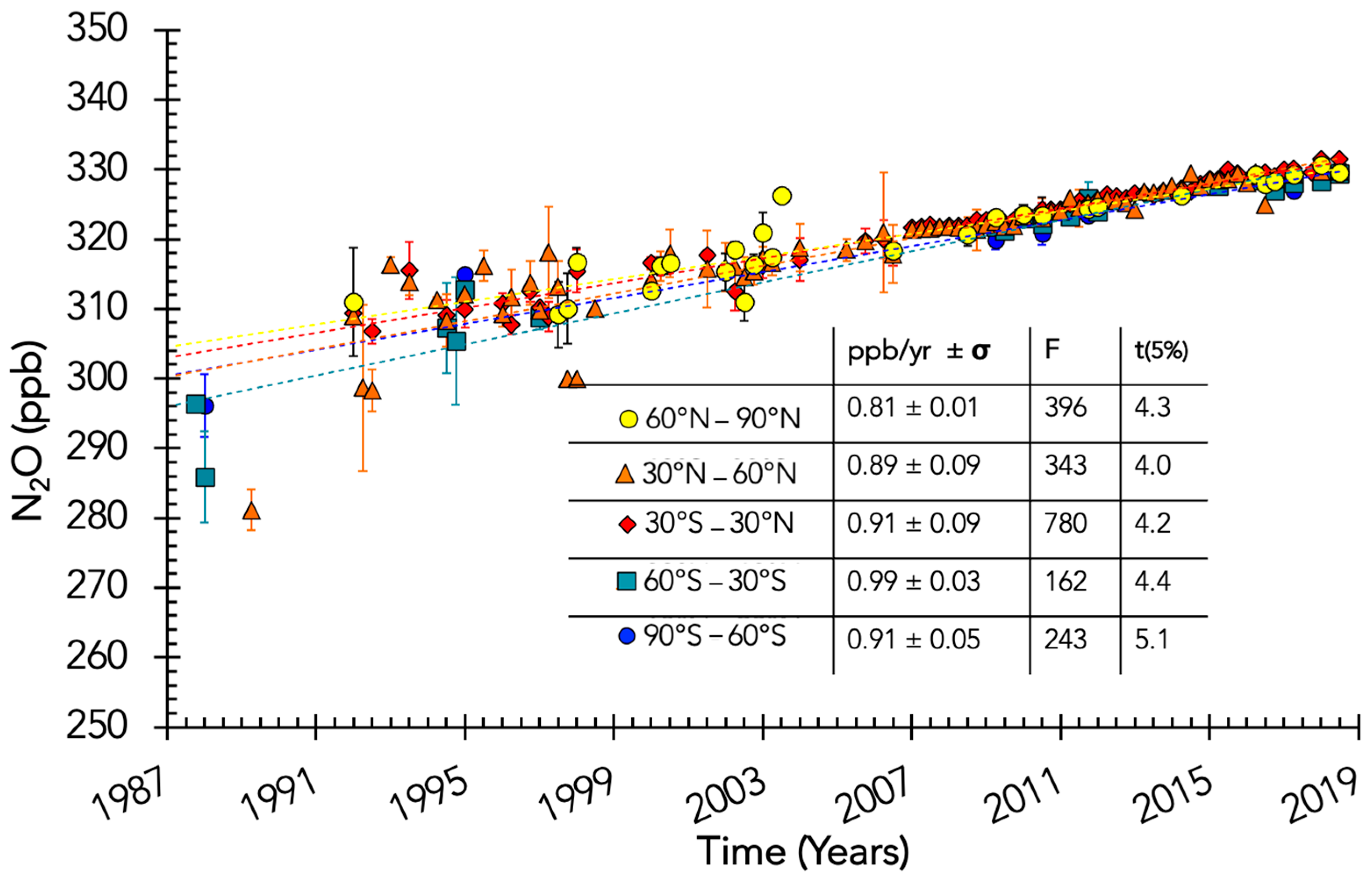
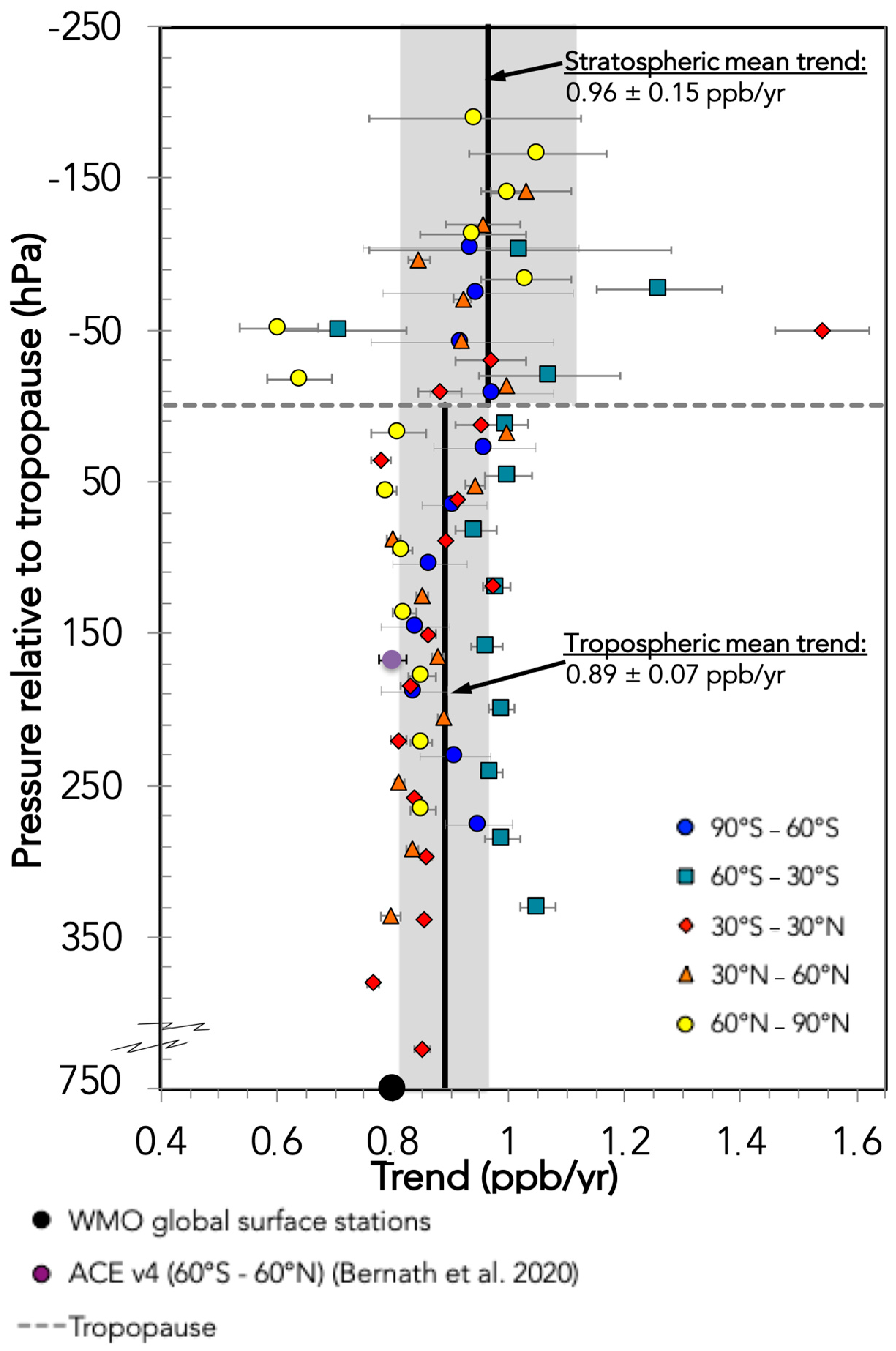
3.1. N₂O Trend in the UTLS

As explained in Section 2.3, N₂O concentrations versus time are calculated for each pressure level and each of the five latitude bins (30° or 60° range) shown in the figure. The slopes of the concentration versus time plots (a linear trend is applied for the entire period) are extracted, taking into account the standard deviation of each bin, the statistical coefficient F (Fisher’s test), and the critical t-value at 95% confidence. The slope in ppb/yr is retained only if the coefficient F is higher than the critical t-value. The more the F value exceeds the critical t-value, the more the trend can be considered linear. The F coefficient and the critical t-value are also shown in Figure 5. Taking into account data from 1987 to 2018 permits validation of the F-test. An example is represented in Figure 5 for a specified pressure range in the upper troposphere (from +20 to +50 hPa compared to the tropopause pressure; see next paragraph for an explanation of the pressure range) for each latitude band described above.

Figure 6 shows the trend of N₂O in ppb per year for all data selected between 1987 and 2018 according to the latitude bands: North and South Polar regions (±[90–60]° N), northern and southern midlatitudes (±[60–30]° N) and tropics (±30°). The vertical axis represents the altitude in pressure relative to the pressure at the tropopause. The tropopause pressure according to latitude has been determined from studies of ERA-interim data from ECMWF [48]. The error bars represent the standard deviation of the slope for the plot concentration versus time (see, e.g., Figure 5). The trends range between 0.8–1.1 ppb/yr in the upper troposphere (up to 350 hPa greater than the tropopause pressure) and 0.64–1.20 ppb/yr in the lower stratosphere (up to 150 hPa less than the tropopause pressure). The data in the stratosphere show more uncertainty, as illustrated by the larger error bar in this part of the atmosphere. Indeed, fewer measurements are available in the stratosphere compared to the troposphere. The average trend is 0.89 ± 0.07 ppb/yr (1σ) in the upper troposphere and 0.96 ± 0.15 ppb/yr (1σ) in the lower stratosphere. Taking into account the uncertainties (one sigma), the difference in the two trends is insignificant. The trend in the southern midlatitude (60–30° S) band seems larger than the others, most visible for pressures relative to the tropopause up to 150 hPa. However, it is important to note that the southern midlatitudes are the least sampled, so lower statistics may also contribute to this difference in the trend.

WMO-reported N₂O average mixing ratio from ground-based AGAGE in situ (Global), NOAA flask and in situ (Global), and CSIRO flask (Global) data [9] is also represented in Figure 6 with a value of 0.80 ppb/yr. Similarly, the mean value of 0.799± 0.024 ppb/yr from the ACE-FTS instrument data on SCISAT [49] is plotted for a band of latitude between 60° S and 60° N and altitudes between 5.5 and 10.5 km, corresponding to a medium pressure of about 170 hPa greater than the tropopause. These ground and upper troposphere trends show consistency with the calculated values within the uncertainties in the troposphere from aircraft and balloon data.

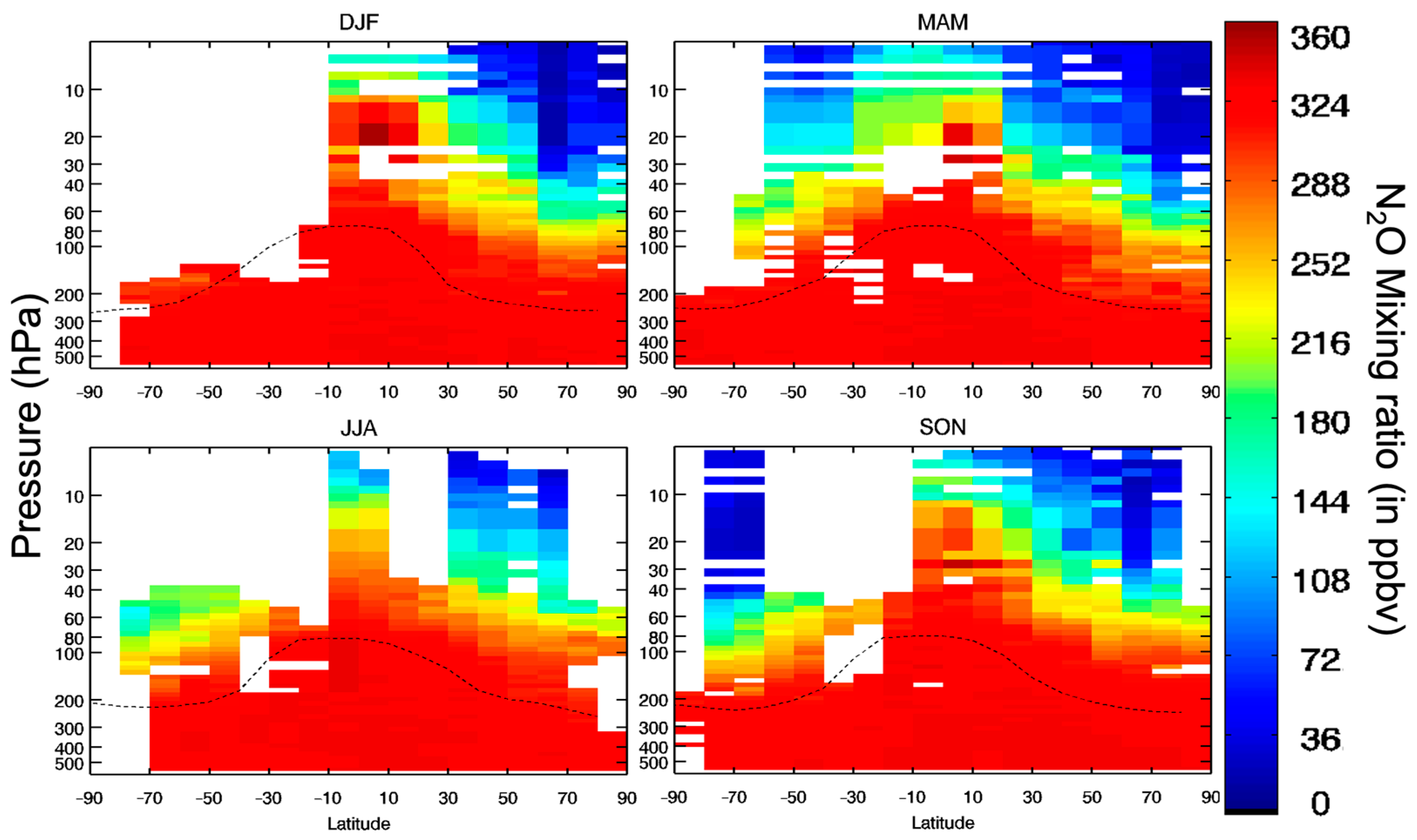
3.2. N₂O Seasonality and Zonal Mean

Figure 7 depicts the zonal mean N₂O binned by latitude and pressure for 2018, including all the data (balloon and aircraft) from 1987 to 2018, which were normalized to 2018 for DJF, MAM, JJA, and SON. For that normalization, the average trend observed in the troposphere in Figure 6 of 0.89 ppb/yr is used to calculate the N₂O concentration for each measurement and adjusted to 2018 as explained in Section 2.3, Equation (5). Then, considering the adjusted datasets, instrumental error-weighted averages are calculated in latitude boxes of 10° width (for all longitudes) and 60 pressure levels (from 600 hPa to 5 hPa). The dataset shows good coverage of latitudes, except for high southern latitudes (above 60° S) in DJF, MAM, and JJA. N₂O concentrations vary between 320 and 340 ppb throughout the troposphere. This observation is consistent with the location of N₂O sources, mainly at the surface (biological sources from soil and water, and anthropogenic sources mainly agricultural soil and animals breeding) and sinks present in the stratosphere (photodissociation and reaction with excited oxygen atoms, O(¹D)), see [50] and reference therein. As observed in the study of Kuttippurath et al. [12], which shows N₂O zonal means for ASUR data, the influence of the stratospheric transport on the N₂O zonal mean is also visible. Indeed, the N₂O VMR (volume mixing ratio) in DJF in the northern latitude (>60° N) stratosphere is lower (180 ppbv around 60 hPa and 10 ppbv around 10 hPa) compared to the other seasons (around 230 ppbv at 60 hPa for JJA), indicating diabatic descent of air in the polar vortex in the winter season (e.g., [51,52]). High concentrations in the lower tropical stratosphere from 100 to 20 hPa predominantly during the northern winter season (DJF) compared to the summer season (JJA) suggest an increase of the tropical upwelling during this season due to Brewer–Dobson circulation. A maximum in tropical upwelling in the DJF season was previously suggested based on trace gas observations and radiative–dynamical calculations ([53] and references therein). The same references predict a minimum in upwelling in the JJA season, as also observed in Figure 7.

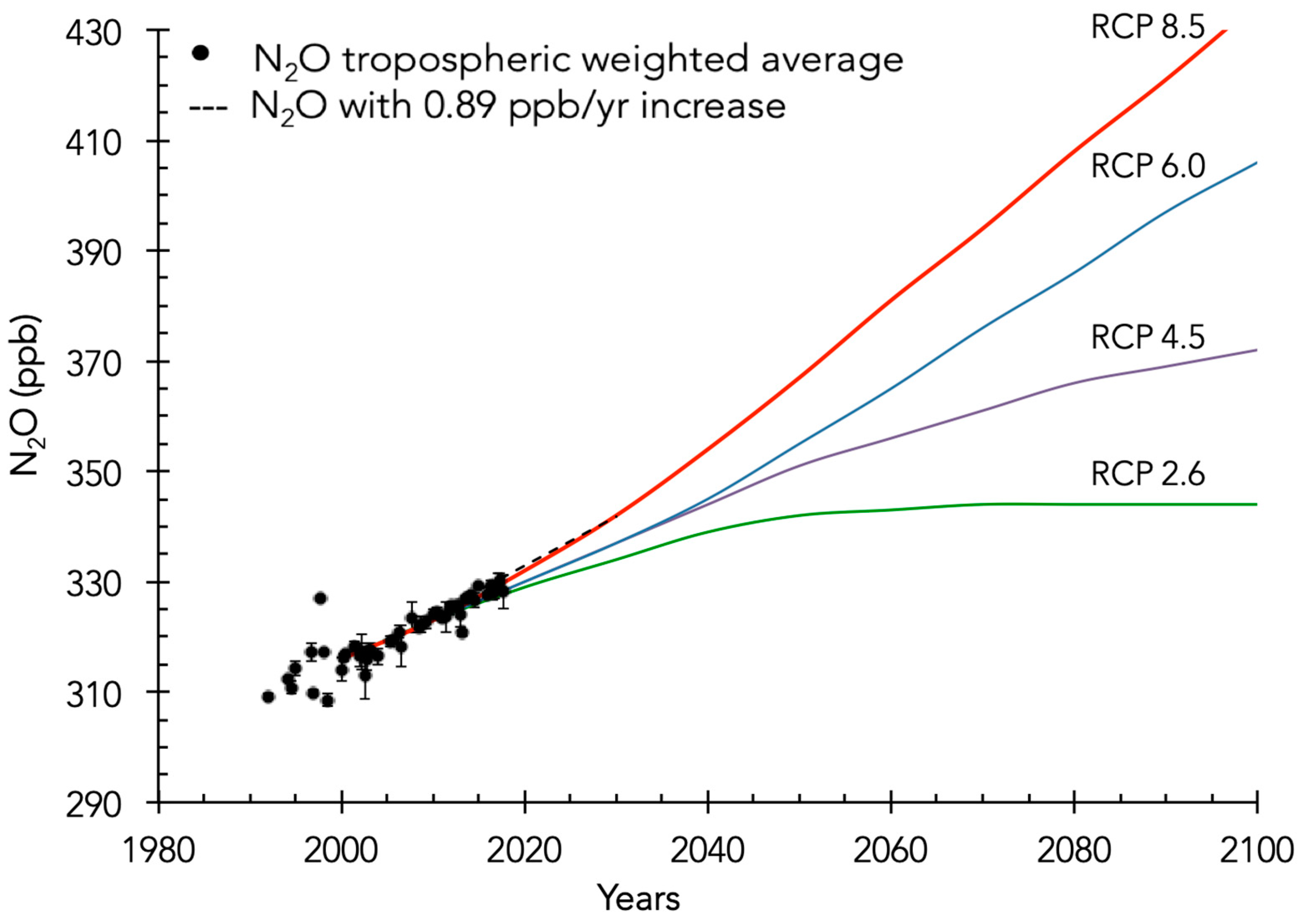
3.3. Discussion Relative to Atmospheric Circulation and Trends

Studies have shown that changes in the Brewer–Dobson circulation (BDC) impact both long-lived and short-term trends in the variability of stratospheric chemical tracers such as HCl and N₂O. Recently, one of these studies identified an increase in the concentration of the long-lived trace gas HCl in the Northern Hemisphere (NH) midlatitude stratosphere from 2005 to 2011, despite well-documented decreases in surface emissions of organic chlorine-containing gases over this period [54]. A chemical transport model (CTM) driven by ERA-interim reanalysis meteorological fields suggested that this short-term HCl trend occurred over several consecutive years, transporting older stratospheric air characterized by the larger relative conversion of organic chlorine-containing source gases to HCl from the upper stratosphere to the lower stratosphere. With regard to N₂O, the suggested enhanced downwelling branch of the residual circulation in the Northern Hemisphere (NH) transports more N₂O-poor air from the upper stratosphere to the lower stratosphere [55] as discussed in Section 3.2. In addition to suggesting the modification of the NH circulation, this study also suggested a weakened downwelling and enhanced poleward flow in the Southern Hemisphere (SH), which brought more low-latitude air to the SH middle latitudes. Unfortunately, due to the lack of N₂O measurements in the SH at some seasons, this part cannot be supported conclusively by our analysis.

Therefore, decadal-scale dynamical variability can have distinct and different impacts on hemispheric long-lived chemical tracers’ variability and trends. Observed hemispheric asymmetry in stratospheric trends is also discussed in [56]. This work used 25 years of column observations from the Network for the Detection of Atmospheric Composition Change (NDACC), along with the above-mentioned Aura MLS observations and the CTM results driven by Modern-Era Retrospective analysis for Research and Applications Version (MERRA2). The results from this work showed extratropical variability with a 5- to 7-year period driven by interactions of the atmospheric circulation and the quasi-biennial oscillation in tropical winds. This previous “unrecognized variability” is large relative to hemispheric transport trends and may bias regression trends of stratospheric species.

4. Summary and Outlook

This paper presents the first compilation of the majority of existing N₂O balloon and aircraft measurements performed between 1987 and 2018, ranging from the middle troposphere to the middle stratosphere. First, we pre-processed the data by blind source separation to exclude particular dynamic cases and outliers. This approach avoids the need for binning the data by latitude and longitude to identify anomalous profiles. With this dataset, we calculated instrumental error-weighted averages in boxes over a wide range of latitudes (North and South Pole, midlatitudes, tropics) and over 10° latitude boxes for pressure levels ranging from 600 hPa to 5 hPa. We extracted trends between 1987 and 2018 (a linear trend is applied for the entire period) and revealed an increase in N₂O concentration of 0.89 ± 0.07 ppb/yr in the upper troposphereand 0.96 ± 0.15 ppb/yr in the lower stratosphere. The growth of this potent greenhouse gas, as observed at the ground and remotely by satellites, is confirmed in situ in the UTLS, the most important region of the atmosphere for the Earth’s radiative balance. We extracted the zonal mean from the whole dataset and illustrated its evolution with seasons DJF, MAM, JJA, and SON. The N₂O zonal mean highlights, as explained in other studies, the atmospheric circulation, with an increase in tropical upwelling during DJF and stratospheric polar descent during northern (or boreal) winter.

With the decrease in halocarbon concentrations, N₂O emissions will become the primary ozone-depleting substance in the future [6]. However, the impact of N₂O depends on the levels of CO₂ and, to a lesser extent, CH₄ [57,58]. The reactivity of N₂O depends largely on the temperature of the stratosphere, and increasing CO₂ (and CH₄) cools the stratosphere [59]. Therefore, it is difficult to quantify the impact of increasing N₂O on ozone depletion without accounting for CO₂ and CH₄. Figure 8 shows the concentration of N₂O in the troposphere between 1987 and 2018 from aircraft and balloon measurements from our study and from Representative Concentration Pathways (RCP) scenarios [60]. The N₂O concentration with an increase of 0.89 ppb/yr (as observed in the troposphere in our study) is also shown. If N₂O emission levels remain constant, the concentrations follow the RCP 6.0 or 8.5 scenarios. According to the study by Revell et al. [58] (in Figure 1), the CO₂ and CH₄ levels with the RCP 6,0 scenario result in ozone depletion potentials (ODP) of 0.019 for N₂O and, therefore, comparable potential as the actual ODP (0.017) as suggested by [6]. Only the anthropogenic emissions part is controllable, and most of this comes from fertilizers used in agriculture, which are difficult to substitute. Models can address the question of the anthropogenic component of the observed N₂O increase. In addition, climate change may also affect the natural part of the emissions, which is difficult to predict.

The role of the “changing” Brewer–Dobson circulation (BDC) in affecting the transport, mixing, and chemistry of long-lived trace gases must be assessed for quantifying the future ozone recovery and, therefore, the estimated return date to a condition before the 1987 Montreal Protocol on Substances that Deplete the Ozone Layer was established [61]. Recently, Minganti et al. [62] examined the impact of the BDC on the N₂O budget in a chemistry–climate model (CCM) and CTM driven with dynamical reanalysis. This analysis used the transformed Eulerian mean (TEM) framework, specifically using the tracer continuity equation derived from the TEM formula to examine the N₂O climatological (2005–2014) seasonal means and climatological annual cycles of the vertical residual advection and the horizontal mixing in these models. A follow-up study evaluated the N₂O rate of change to understand the stratospheric Brewer–Dobson circulation in a CCM [63]. This study used both FTIR ground-based and ACE-FTS observations. Our work provides for the robust inclusion of MTMS airborne and balloon-borne observations to understand further the dynamical processes that control BDC and how these processes will affect N₂O distributions in a future climate

References

1. Prather, M.J.; Hsu, J.; DeLuca, N.M.; Jackman, C.H.; Oman, L.D.; Douglass, A.R.; Fleming, E.L.; Strahan, S.E.; Steenrod, S.D.; Sovde, O.A.; et al. Measuring and modelling the lifetime of nitrous oxide including its variability. J. Geophys. Res. Atmos. 2015, 120, 5693–5705. [Google Scholar] [CrossRef]
2. Ravishankara, A.R.; Pele, A.-L.; Zhou, L.; Ren, Y.; Zogka, A.; Daele, V.; Idir, M.; Brown, S.S.; Romanias, M.N.; Mellouki, A. Atmospheric loss of nitrous oxide (N2O) is not influenced by its potential reactions with OH and NO3 radicals. Phys. Chem. Chem. Phys. 2019, 21, 24592–24600. [Google Scholar] [CrossRef]
3. Myhre, G.; Shindell, D.T. Anthropogenic and Natural Radiative Forcing, Chapter 8. In Climate Change 2013: The Physical Science Basis; Contribution of Working Group I to the Fifth Assessment Report of the Intergovernmental Panel on Climate Change; Jacob, D.J., Ravishankara, A.R., Shine, K., Eds.; Cambridge University Press: Cambridge, UK, 2013; pp. 659–740. [Google Scholar]
4. Ciais, P.; Sabine, C.; Bala, G.; Bopp, L.; Brovkin, V.; Canadell, J.; Chhabra, A.; DeFries, R.; Galloway, J.; Heimann, M.; et al. Carbon and Other Biogeochem. Cy. In Climate Change 2013: The Physical Science Basis; Contribution of Working Group I to the Fifth Assessment Report of the Intergovernmental Panel on Climate Change; Stocker, T.F., Qin, D., Plattner, G.-K., Tignor, M., Allen, S.K., Boschung, J., Nauels, A., Xia, Y., Bex, V., Midgley, P.M., Eds.; Cambridge University Press: Cambridge, UK; New York, NY, USA, 2013. [Google Scholar]
5. Crutzen, P. A Review of Upper Atmospheric Photochemistry. Can. J. Chem. 1974, 52, 1569–1581. [Google Scholar] [CrossRef] [Green Version]
6. Ravishankara, A.R.; Daniel, J.S.; Portmann, R.W. Nitrous oxide (N2O): The dominant ozone-depleting substance emitted in the 21st century. Science 2009, 326, 123–125. [Google Scholar] [CrossRef] [Green Version]
7. Brasseur, G.P.; Solomon, S. Aeronomy of the Middle Atmosphere, 3rd ed.; Springer: Dordrecht, The Netherlands, 2005; p. 664. [Google Scholar]
8. Elkins, J.W.; Dutton, G.S. Nitrous oxide and sulfur hexafluoride in ‘State of the Climate in 2008. Bull. Am. Meteoro-Log. Soc. 2009, 90, S38–S39. [Google Scholar] [CrossRef] [Green Version]
9. Engel, A.; Rigby, M.; Burkholder, J.B.; Fernandez, R.P.; Froidevaux, L.; Hall, B.D.; Hossaini, R.; Saito, T.; Vollmer, M.K.; Yao, B. Update on Ozone-Depleting Substances (ODSs) and other gases of interest to the Montreal Protocol, Chapter 1. In Scientific Assessment of Ozone Depletion: 2018, Global Ozone Research and Monitoring; Project–Report No. 58; World Meteorological Organization: Geneva, Switzerland, 2018. [Google Scholar]
10. Webster, C.R.; May, R.D.; Trimble, C.; Chave, R.G.; Kendall, J.E. Aircraft (ER-2) laser infrared absorption spectrometer (ALIAS) for in-situ stratospheric measurements of HCI, N(2)O, CH(4), NO(2), and HNO(3). Appl. Opt. 1994, 33, 454–472. [Google Scholar] [CrossRef]
11. Loewenstein, M.; Jost, H.; Grose, J.; Eilers, J.; Lynch, D.; Jensen, S.; Marmie, J. Argus: A new instrument for the measurement of the stratospheric dynamical tracers, N2O and CH4. Spectrochim. Acta A 2002, 58, 2329–2345. [Google Scholar] [CrossRef]
12. Kuttippurath, J.; Kleinböhl, A.; Bremer, H.; Küllmann, H.; Notholt, J.; Sinnhuber, B.-M.; Feng, W.; Chipperfield, M. Aircraft measurements and model simulations of stratospheric ozone and N2O: Implications for chemistry and transport processes in the models. J. Atmos. Chem. 2010, 66, 41–64. [Google Scholar] [CrossRef]
13. Podolske, J.; Loewenstein, M. Airborne tunable diode laser spectrometer for trace-gas measurement in the lower strato-sphere. Appl. Opt. 1993, 32, 5324–5333. [Google Scholar] [CrossRef] [PubMed]
14. Farmer, C.B. High resolution infrared spectroscopy of the Sunand the Earth’s atmosphere from space. Mikrochim. Acta 1987, 3, 189–214. [Google Scholar] [CrossRef]
15. Sachse, G.W.; Hill, G.F.; Wade, L.O.; Perry, M.G. Fast-response, high-precision carbon monoxide sensor using a tunable diode laser absorption technique. J. Geophys. Res. 1987, 92, 2071–2081. [Google Scholar] [CrossRef]
16. Jucks, K.W.; Johnson, D.G.; Chance, K.V.; Traub, W.A.; Margitan, J.J.; Osterman, G.B.; Salawitch, R.J.; Sasano, Y. Observations of OH, HO2, H2O, and O3 in the upper stratosphere: Implications for HOx photochemistry. Geophys. Res. Lett. 1998, 25, 3935–3938. [Google Scholar] [CrossRef] [Green Version]
17. Friedl-Vallon, F.; Maucher, G.; Kleinert, A.; Lengel, A.; Keim, C.; Oelhaf, H.; Fischer, H.; Seefeldner, M.; Trieschmann, O. Design and characterization of the balloon-borne Michelson Interferometer for Passive Atmospheric Sounding (MIPAS-B2). Appl. Opt. 2004, 43, 3335–3355. [Google Scholar] [CrossRef]
18. Toon, G.C. The JPL MkIV Interferometer. Opt. Photonics News 1991, 2, 19–21. [Google Scholar] [CrossRef]
19. Kort, E.A.; Patra, P.K.; Ishijima, K.; Daube, B.C.; Jiménez, R.; Elkins, J.; Hurst, D.; Moore, F.L.; Sweeney, C.; Wofsy, S.C. Tropospheric distribution and variability of N2O: Evidence for strong tropical emissions. Geophys. Res. Lett. 2011, 38, L15806. [Google Scholar] [CrossRef] [Green Version]
20. Santoni, G.W.; Daube, B.C.; Kort, E.A.; Jiménez, R.; Park, S.; Pittman, J.V.; Gottlieb, E.; Xiang, B.; Zahniser, M.S.; Nelson, D.D.; et al. Evaluation of the airborne quantum cascade laser spectrometer (QCLS) measurements of the carbon and greenhouse gas suite–CO2, CH4, N2O, and CO–during the CalNex and HIPPO campaigns. Atmos. Meas. Tech. 2014, 7, 1509–1526. [Google Scholar] [CrossRef] [Green Version]
21. Commane, R.; Budney, J.W.; Gonzalez Ramos, Y.; Sargent, M.; Wofsy, S.C.; Daube, B.C. ATom: Measurements from the Quantum Cascade Laser System (QCLS); Version 2; ORNL DAAC: Oak Ridge, TN, USA, 2021. [CrossRef]
22. Gonzalez, Y.; Commane, R.; Manninen, E.; Daube, B.C.; Schiferl, L.D.; McManus, J.B.; McKain, K.; Hintsa, E.J.; Elkins, J.W.; Montzka, S.A.; et al. Impact of stratospheric air and surface emissions on tropospheric nitrous ox-ide during Atom. Atmos. Chem. Phys. 2021, 21, 11113–11132. [Google Scholar] [CrossRef]
23. Stachnik, R.A.; Millán, L.; Jarnot, R.; Monroe, R.; McLinden, C.; Kühl, S.; Puķīte, J.; Shiotani, M.; Suzuki, M.; Kasai, Y.; et al. Stratospheric BrO abundance measured by a balloon-borne submil-limeterwave radiometer. Atmos. Chem. Phys. 2013, 13, 3307–3319. [Google Scholar] [CrossRef] [Green Version]
24. Moreau, G.; Robert, C.; Catoire, V.; Chartier, M.; Camy-Peyret, C.; Huret, N.; Pirre, M.; Pomathiod, L.; Chalumeau, G. SPI-RALE: A multispecies in situ balloonborne instrument with six tunable diode laser spectrometers. Appl. Opt. 2005, 44, 5972–5989. [Google Scholar] [CrossRef] [PubMed]
25. AERIS Datacenter. Available online: https://cds-espri.ipsl.upmc.fr/etherTypo/index.php?id=347&L=1 (accessed on 15 December 2022).
26. Schiller, C.; Bozem, H.; Gurk, C.; Parchatka, U.; Königstedt, R.; Harris, G.; Lelieveld, J.; Fischer, H. Applications of quantum cascade lasers for sensitive trace gas measurements of CO, CH4, N2O and HCHO. Appl. Phys. B 2008, 92, 419–430. [Google Scholar] [CrossRef]
27. Müller, S.; Hoor, P.; Bozem, H.; Gute, E.; Vogel, B.; Zahn, A.; Bönisch, H.; Keber, T.; Krämer, M.; Rolf, C.; et al. Impact of the Asian monsoon on the extratropical lower stratosphere: Trace gas observations during TACTS over Europe 2012. Atmos. Chem. Phys. 2016, 16, 10573–10589. [Google Scholar] [CrossRef] [Green Version]
28. Krause, J.; Hoor, P.; Engel, A.; Plöger, F.; Grooß, J.-U.; Bönisch, H.; Keber, T.; Sinnhuber, B.-M.; Woiwode, W.; Oelhaf, H. Mixing and ageing in the polar lower stratosphere in winter 2015–2016. Atmos. Chem. Phys. 2018, 18, 6057–6073. [Google Scholar] [CrossRef] [Green Version]
29. Hoor, P.; Gurk, C.; Brunner, D.; Hegglin, M.I.; Wernli, H.; Fischer, H. Seasonality and extent of extratropical TST derived from in-situ CO measurements during SPURT. Atmos. Chem. Phys. 2004, 4, 1427–1442. [Google Scholar] [CrossRef] [Green Version]
30. Viciani, S.; D’Amato, F.; Mazzinghi, P.; Castagnoli, F.; Toci, G.; Werle, P.A. Cryogenically operated laser diode spectrometer for airborne measurement of stratospheric trace gases. Appl. Phys. B 2008, 90, 581–592. [Google Scholar] [CrossRef]
31. Viciani, S.; Montori, A.; Chiarugi, A.; D’Amato, F. A Portable Quantum Cascade Laser Spectrometer for Atmospheric Meas-urements of Carbon Monoxide. Sensors 2018, 18, 2380. [Google Scholar] [CrossRef] [PubMed] [Green Version]
32. Müller, S.; Hoor, P.; Berkes, F.; Bozem, H.; Klingebiel, M.; Reutter, P.; Smit, H.G.J.; Wendisch, M.; Spichtinger, P.; Borrmann, S. In situ detection of stratosphere-troposphere exchange of cirrus particles in the midlatitudes. Geophys. Res. Lett. 2015, 42, 949–955. [Google Scholar] [CrossRef]
33. Kunkel, D.; Hoor, P.; Kaluza, T.; Ungermann, J.; Kluschat, B.; Giez, A.; Lachnitt, H.C.; Kaufmann, M.; Riese, M. Evidence of small-scale quasi-isentropic mixing in ridges of extratropical baroclinic waves. Atmos. Chem. Phys. 2019, 19, 12607–12630. [Google Scholar] [CrossRef] [Green Version]
34. Elkins, J.W.; Fahey, D.W.; Gilligan, J.M.; Dutton, G.S.; Baring, T.J.; Volk, C.M.; Dunn, R.E.; Myers, R.C.; Montzka, S.A.; Wamsley, P.R.; et al. Airborne gas chromatograph for in situ measurements of long-lived species in the upper troposphere and lower stratosphere. Geophys. Res. Lett. 1996, 23, 347–350. [Google Scholar] [CrossRef] [Green Version]
35. Romashkin, P.A.; Hurst, D.F.; Elkins, J.W.; Dutton, G.S.; Fahey, D.W.; Dunn, R.E.; Moore, F.L.; Myers, R.C.; Hall, B.D. In Situ Measurements of Long-Lived Trace Gases in the Lower Stratosphere by Gas Chromatography. J. Atmos. Ocean. Technol. 2001, 18, 1195–1204. [Google Scholar] [CrossRef]
36. Hintsa, E.J.; Moore, F.L.; Hurst, D.F.; Dutton, G.S.; Hall, B.D.; Nance, J.D.; Miller, B.R.; Montzka, S.A.; Wolton, L.P.; McClure-Begley, A.; et al. UAS Chromatograph for Atmospheric Trace Species (UCATS)—A versatile instrument for trace gas measurements on airborne platforms. Atmos. Meas. Tech. 2021, 14, 6795–6819. [Google Scholar] [CrossRef]
37. Moore, F.L.; Elkins, J.W.; Ray, E.A.; Dutton, G.S.; Dunn, R.E.; Fahey, D.W.; McLaughlin, R.J.; Thompson, T.L.; Romashkin, P.A.; Hurst, D.F.; et al. Balloonborne in situ gas chromatograph for measurements in the troposphere and stratosphere. J. Geophys. Res. 2003, 108, 8330. [Google Scholar] [CrossRef]
38. Moore, F.; Dutton, G.; Elkins, J.W.; Hall, B.; Hurst, D.; Nance, J.D.; Thompson, T. PANTHER Data from SOLVE-II through CR-AVE: A Contrast between Long- and Short-Lived Compounds. Am. Geophys. Union 2006, 2006, A41A-0025. [Google Scholar]
39. Blake, N.J.; Blake, D.R.; Simpson, I.J.; Meinardi, S.; Swanson, A.L.; Lopez, J.P.; Katzenstein, A.S.; Barletta, B.; Shirai, T.; Atlas, E.; et al. NMHCs and halocarbons in Asian continental outflow during the Transport and Chemical Evolution over the Pacific (TRACE-P) field campaign: Comparison with PEM-West B. J. Geophys. Res. 2003, 108, 8806. [Google Scholar] [CrossRef] [Green Version]
40. Heidt, L.E.; Vedder, J.F.; Pollock, W.H.; Lueb, R.A.; Henry, B.E. Trace gases in the Antarctic atmosphere. J. Geophys. Res. 1989, 94, 11599. [Google Scholar] [CrossRef]
41. Schauffler, S.M.; Atlas, E.L.; Blake, D.R.; Flocke, F.; Lueb, R.A.; Lee-Taylor, J.M.; Stroud, V.; Travnicek, W. Distributions of brominated organic compounds in the troposphere and lower stratosphere. J. Geophys. Res. 1999, 104, 21513–21535. [Google Scholar] [CrossRef] [Green Version]
42. Montzka, S.; Moore, F.; Sweeney, C. ATom: L2 Measurements from the Programmable Flask Package (PFP) Whole Air Sampler; ORNL DAAC: Oak Ridge, TN, USA, 2019. [CrossRef]
43. Sweeney, C.; Karion, A.; Wolter, S.; Newberger, T.; Guenther, D.; Higgs, J.A.; Andrews, A.E.; Lang, P.M.; Neff, D.; Dlugokencky, E.; et al. Seasonal climatology of CO2 across North America from aircraft measurements in the NOAA/ESRL Global Greenhouse Gas Reference Network. J. Geophys. Res. D Atmos. 2015, 120, 5155–5190. [Google Scholar] [CrossRef]
44. Kaiser, J.; Engel, A.; Borchers, R.; Röckmann, T. Probing stratospheric transport and chemistry with new balloon and aircraft observations of the meridional and vertical N2O isotope distribution. Atmos. Chem. Phys. 2006, 6, 3535–3556. [Google Scholar] [CrossRef] [Green Version]
45. Schuck, T.J.; Brenninkmeijer, C.A.M.; Slemr, F.; Xueref-Remy, I.; Zahn, A. Greenhouse gas analysis of air samples col-lectedonboard the CARIBIC passenger aircraft. Atmos. Meas. Tech. 2009, 2, 449–464. [Google Scholar] [CrossRef] [Green Version]
46. Comon, P.; Jutten, C. Handbook of Blind Source Separation: Independent Component Analysis and Blind Deconvolution; Academic Press: Oxford, UK, 2010. [Google Scholar]
47. Bretherton, C.S.; Smith, C.; Wallace, J.M. An Intercomparison of Methods for Finding Coupled Patterns in Climate Data. J. Clim. 1992, 5, 541–560. [Google Scholar] [CrossRef]
48. Wilcox, L.J.; Hoskins, B.J.; Shine, K.P. A global blended tropopause based on ERA data. Part I: Climatology. Q. J. R. Meteorol. Soc. 2012, 138, 561–575. [Google Scholar] [CrossRef] [Green Version]
49. Bernath, P.F.; McElroy, C.T.; Abrams, M.C.; Boone, C.D.; Butler, M.; Camy-Peyret, C.; Carleer, M.; Clerbaux, C.; Coheur, P.-F.; Colin, R.; et al. Aeronomy of the Middle Atmosphere, 3rd ed.; Springer: Dordrecht, The Netherlands, 2005; p. 644. [Google Scholar]
50. Seinfeld, J.H.; Pandis, S.N. Atmospheric Chemistry and Physics: From Air Pollution to Climate Change, 3rd ed.; Wiley & Sons, Inc.: Hoboken, NJ, USA, 2016. [Google Scholar]
51. Bremer, H.; von König, M.; Kleinböhl, A.; Küllmann, H.; Künzi, K.; Bramstedt, K.; Burrows, J.P.; Eichmann, K.-U.; Weber, M.; Goede, A.P.H. Ozone depletion observed by ASUR during the Arctic winter 1999/2000. J. Geophys. Res. 2002, 107, 8277. [Google Scholar] [CrossRef]
52. Greenblatt, J.B.; Jost, H.-J.; Loewenstein, M.; Podolske, J.R.; Hurst, D.F.; Elkins, J.W.; Schauffler Atlas, E.L.; Herman, R.L.; Webster, C.R.; Bui, T.P.; et al. Tracer-based determination of vortex descent in the 1999/2000 Arctic winter. J. Geophys. Res. 2002, 107, 8279. [Google Scholar] [CrossRef] [Green Version]
53. Niwano, M.; Yamazaki, K.; Shiotani, M. Seasonal and QBO variations of ascent rate in the tropical lower stratosphere as inferred from UARS HALOE trace gas data. J. Geophys. Res. 2003, 108, 4794. [Google Scholar] [CrossRef] [Green Version]
54. Mahieu, E.; Chipperfield, M.; Notholt, J.; Reddmann, J.T.; Anderson, J.; Bernath, P.F.; Blumenstock, T.; Coffey, M.T.; Dhomse, S.S.; Feng, W.; et al. Recent Northern Hemisphere stratospheric HCl increase due to atmospheric circulation changes. Nature 2015, 515, 104–107. [Google Scholar] [CrossRef] [Green Version]
55. Han, Y.; Tian, W.; Chipperfield, M.P.; Zhang, J.; Wang, F.; Sang, W.; Luo, J.; Feng, W.; Chrysanthou, A.; Tian, H. Attribution of the hemispheric asymmetries in trends of stratospheric trace gases inferred from Microwave Limb Sounder (MLS) meas-urements. J. Geophys. Res. Atmos. 2019, 124, 6283–6293. [Google Scholar] [CrossRef]
56. Strahan, S.E.; Smale, D.; Douglass, A.R.; Blumenstock, T.; Hannigan, J.W.; Hase, F.; Jones, N.B.; Mahieu, E.; Notholt, J.; Oman, L.D.; et al. Observed hemispheric asymmetry in stratospheric transport trends from 1994 to 2018. Geophys. Res. Lett. 2020, 47, e2020GL088567. [Google Scholar] [CrossRef]
57. Portmann, R.W.; Daniel, J.S.; Ravishankara, A.R. Stratospheric ozone depletion due to nitrous oxide: Influences of other gases. Philos. Trans. R. Soc. Lond. B Biol. Sci. 2012, 367, 1256–1264. [Google Scholar] [CrossRef] [PubMed] [Green Version]
58. Revell, L.; Bodeker, G.; Huck, P.; Williamson, B.; Rozanov, E. The sensitivity of stratospheric ozone changes through the 21st century to N2O and CH4. Atmos. Chem. Phys. 2012, 12, 11309–11317. [Google Scholar] [CrossRef] [Green Version]
59. Rosenfield, J.E.; Douglass, A.R. Doubled CO2 effects on NOy in a coupled 2D model. Geophys. Res. Lett. 1998, 25, 4381–4384. [Google Scholar] [CrossRef]
60. IPCC (Intergovernmental Panel on Climate Change). 2022: Climate Change 2022: Mitigation of Climate Change; Working Group III Contribution to the IPCC Sixth Assessment Report; Cambridge University Press: Cambridge, UK, 2022. [Google Scholar]
61. Dhomse, S.S.; Kinnison, D.; Chipperfield, M.P.; Salawitch, R.J.; Cionni, I.; Hegglin, M.I.; Abraham, N.L.; Akiyoshi, H.; Archibald, A.T.; Bednarz, E.M.; et al. Esti-mates of ozone return dates from Chemistry-Climate Model Initiative simulations. Atmos. Chem. Phys. 2018, 18, 8409–8438. [Google Scholar] [CrossRef] [Green Version]
62. Minganti, D.; Charillat, S.; Christophe, Y.; Errera, Q.; Abalos, M.; Prignon, M.; Kinnison, D.E.; Mahieu, E. Climatological impact of the Brewer-Dobson circulation on the N2O budget in WACCM, a chemical reanalysis and a CTM driven by four dynamical reanalysis. Atmos. Chem. Phys. 2020, 20, 12609–12631. [Google Scholar] [CrossRef]
63. Minganti, D.; Chabrillat, S.; Errera, Q.; Prignon, M.; Kinnison, D.E.; Garcia, R.R.; Abalos, M.; Alsing, J.; Schneider, M.; Smale, D.; et al. Evaluation of the N2O rate of change to understand the stratospheric Brewer-Dobson circulation in a Chemistry-Climate Model. J. Geophys. Res. Atmos. 2022, 127, e2021JD036390. [Google Scholar] [CrossRef] [PubMed]
64. AAOE Website. Available online: https://csl.noaa.gov/projects/aaoe/ (accessed on 15 December 2022).
65. AASE Website. Available online: https://espo.nasa.gov/aase/ (accessed on 15 December 2022).
66. OMS Website. Available online: https://espoarchive.nasa.gov/archive/browse/oms/Balloon (accessed on 15 December 2022).
67. Hoell, J.M.; Davis, D.D.; Liu, S.C.; Newell, R.; Shipham, M.; Akimoto, H.; McNeal, R.J.; Bendura, R.J.; Drewry, J.W. Pacific Exploratory Mission-West A (PEM-West A): September–October 1991. J. Geophys. Res. 1996, 101, 1641–1653. [Google Scholar] [CrossRef]
68. AASE2 Website. Available online: https://espo.nasa.gov/aase2 (accessed on 15 December 2022).
69. SPADE Website. Available online: https://espo.nasa.gov/spade/content/SPADE (accessed on 15 December 2022).
70. Gunson, M.R.; Abbas, M.M.; Abrams, M.C.; Allen, M.; Brown, L.R.; Brown, T.L.; Chang, A.Y.; Goldman, A.; Irion, F.W.; Lowes, L.L.; et al. The Atmospheric Trace Molecule Spectroscopy (ATMOS) Experiment: Deployment on the ATLAS space shuttle missions. Geophys. Res. Lett. 1996, 23, 1569. [Google Scholar] [CrossRef] [Green Version]
71. Engel, A.; Schmidt, U.; Stachnik, R.A. Partitioning Between Chlorine Reservoir Species Deduced from Observations in the Arctic Winter Stratosphere. J. Atmos. Chem. 1997, 27, 107–126. [Google Scholar] [CrossRef]
72. Tuck, A. Introduction to special section: ASHOE/MAESA. J. Geophys. Res. 1997, 102, 3899. [Google Scholar] [CrossRef]
73. Hoell, J.M.; Davis, D.D.; Liu, S.C.; Newell, R.; Akimoto, H.; McNeal, R.J.; Bendura, R.J. The Pacific Exploratory Mission-West Phase B: February–March 1994. J. Geophys. Res. 1997, 102, 28223–28239. [Google Scholar] [CrossRef]
74. Flocke, F.; Herman, R.L.; Salawitch, R.J.; Atlas, E.L.; Webster, C.R.; Schauffler, S.M.; Lueb, R.A.; May, R.D.; Moyer, E.J.; Rosenlof, K.H.; et al. An examination of the chemistry and transport processes in the tropical lower stratosphere using observations of long-lived and short-lived compounds obtained during STRAT and POLARIS. J. Geophys. Res. 1999, 26, 625–642. [Google Scholar] [CrossRef]
75. STRAT Website. Available online: https://espo.nasa.gov/strat/ (accessed on 15 December 2022).
76. Andreae, M.O.; Fishman, J.; Lindesay, J. The Southern Tropical Atlantic Region Experiment (STARE): Transport and At-mospheric Chemistry near the Equator--Atlantic (TRACE A) and Southern African Fire-Atmosphere Research Initiative (SAFARI): An introduction. J. Geophys. Res. 1996, 101, 519–520. [Google Scholar] [CrossRef]
77. Newman, P.A.; Fahey, D.W.; Brune, W.H.; Kurylo, M.J.; Kawa, S.R. Preface [to special section on Photochemistry of Ozone Loss in the Arctic Region in Summer (POLARIS)]. J. Geophys. Res. 1999, 104, 26481–26495. [Google Scholar] [CrossRef]
78. Fuelberg, H.; Newell, R.E.; Westberg, D.J.; Maloney, J.C.; Hannan, J.R.; Martin, B.D.; Avery, M.A.; Zhu, Y. A meteorological overview of the second Pacific Exploratory Mission in the Tropics. J. Geophys. Res. 2001, 106, 427–443. [Google Scholar] [CrossRef] [Green Version]
79. Newman, P.A.; Harris, N.R.; Adriani, A.; Amanatidis, G.T.; Anderson, J.G.; Braathen, G.O.; Brune, W.H.; Carslaw, K.S.; Craig, M.S.; DeCola, P.L.; et al. An overview of the SOLVE/THESEO 2000 campaign. J. Geophys. Res. 2002, 107, 8259. [Google Scholar] [CrossRef] [Green Version]
80. Hurst, D.F.; Schauffler, S.M.; Greenblatt, J.B.; Jost, H.; Herman, R.L.; Elkins, J.W.; Romashkin, P.A.; Atlas, E.L.; Donnelly, S.G.; Podolske, J.R.; et al. The Construction of a Unified, High-Resolution Nitrous Oxide Data Set for ER-2 Flights During SOLVE. J. Geophys. Res. 2002, 107, 8271. [Google Scholar] [CrossRef]
81. SOLVE Website. Available online: https://espo.nasa.gov/solve/ (accessed on 15 December 2022).
82. Urban, J.; Lautié, N.; Le Flochmoen, E.; Jimenez, C.; Eriksson, P.; de La Noë, J.; Dupuy, E.; El Amraoui, L.; Frisk, U.; Jégou, F.; et al. Odin/SMR limb observations of stratospheric trace gases: Validation of N2O. J. Geophys. Res. Atmos. 2005, 110, D09301. [Google Scholar] [CrossRef] [Green Version]
83. Jégou, F.; Urban, J.; de La Noë, J.; Ricaud, P.; Le Flochmoën, E.; Murtagh, D.P.; Eriksson, P.; Jones, A.; Petelina, S.; Llewellyn, E.J.; et al. Technical Note: Validation of Odin/SMR limb observations of ozone, comparisons with OSIRIS, POAM III, ground-based and balloon-borne instruments. Atmos. Chem. Phys. 2008, 8, 3385–3409. [Google Scholar] [CrossRef] [Green Version]
84. Jacob, D.J.; Crawford, J.H.; Kleb, M.M.; Connors, V.S.; Bendura, R.J.; Raper, J.L.; Sachse, G.W.; Gille, J.C.; Emmons, L.; Heald, C.L. Transport and Chemical Evolution over the Pacific (TRACE-P) aircraft mission: Design, execution, and first results. J. Geophys. Res. 2003, 108, 9000. [Google Scholar] [CrossRef]
85. Engel, A.; Bönisch, H.; Brunner, D.; Fischer, H.; Franke, H.; Günther, G.; Gurk, C.; Hegglin, M.; Hoor, P.; Königstedt, R.; et al. Highly resolved observations of trace gases in the lowermost stratosphere and upper troposphere from the Spurt project: An overview. Atmos. Chem. Phys. 2006, 6, 283–301. [Google Scholar] [CrossRef] [Green Version]
86. Fix, A.; Ehret, G.; Flentje, H.; Poberaj, G.; Gottwald, M.; Finkenzeller, H.; Bremer, H.; Bruns, M.; Burrows, J.P.; Kleinböhl, A.; et al. SCIAMACHY validation by aircraft remote sensing: Design, execution, and first measurement results of the SCIA-VALUE mission. Atmos. Chem. Phys. 2005, 5, 1273–1290. [Google Scholar] [CrossRef] [Green Version]
87. BOS Website. Available online: https://espoarchive.nasa.gov/archive/browse/bos (accessed on 15 December 2022).
88. Laube, J.C.; Engel, A.; Bönisch, H.; Möbius, T.; Worton, D.R.; Sturges, W.T.; Grunow, K.; Schmidt, U. Contribution of very short-lived organic substances to stratospheric chlorine and bromine in the tropics—A case study. Atmos. Chem. Phys. 2008, 8, 7325–7334. [Google Scholar] [CrossRef] [Green Version]
89. Wetzel, G.; Bracher, A.; Funke, B.; Goutail, F.; Hendrick, F.; Lambert, J.-C.; Mikuteit, S.; Piccolo, C.; Pirre, M.; Bazureau, A.; et al. Validation of MIPAS-ENVISAT NO2 operational data. Atmos. Chem. Phys. 2007, 7, 3261–3284. [Google Scholar] [CrossRef] [Green Version]
90. Cortesi, U.; Lambert, J.C.; De Clercq, C.; Bianchini, G.; Blumenstock, T.; Bracher, A.; Castelli, E.; Catoire, V.; Chance, K.V.; De Mazière, M.; et al. Geophysical validation of MIPAS-ENVISAT operational ozone data. Atmos. Chem. Phys. 2007, 7, 4807–4867. [Google Scholar] [CrossRef] [Green Version]
91. Kleinböhl, A.; Kuttippurath, J.; Sinnhuber, M.; Sinnhuber, B.-M.; Küllmann, H.; Künzi, K.; Notholt, J. Rapid meridional transport of tropical airmasses to the Arctic during the major stratospheric warming in January 2003. Atmos. Chem. Phys. 2005, 5, 1291–1299. [Google Scholar] [CrossRef] [Green Version]
92. SOLVE2 Website. Available online: https://espo.nasa.gov/solve2/ (accessed on 15 December 2022).
93. Schoeberl, M.R.; Douglass, A.R.; Joiner, J. Introduction to special section on Aura Validation. J. Geophys. Res. 2008, 113, D15S01. [Google Scholar] [CrossRef] [Green Version]
94. AVE-POLAR. Available online: https://espo.nasa.gov/ave-polar/ (accessed on 15 December 2022).
95. Kleinböhl, A.; Bremer, H.; Küllmann, H.; Kuttippurath, J.; Browell, E.V.; Canty, T.; Salawitch, R.J.; Toon, G.C.; Noholt, J. Dentrification in the Arctic mid-winter 2004/2005 observed by airborne submillimeter radiometry. Geophys. Res. Lett. 2005, 32, L19811. [Google Scholar] [CrossRef] [Green Version]
96. AVE-HOUSTON Website. Available online: https://espo.nasa.gov/ave-houston2 (accessed on 15 December 2022).
97. AVE-COSTARICA Website. Available online: https://espo.nasa.gov/ave-costarica2/ (accessed on 15 December 2022).
98. Singh, H.B.; Brune, W.H.; Crawford, J.H.; Flocke, F.; Jacob, D.J. Chemistry and transport of pollution over the Gulf of Mexico and the Pacific: Spring 2006 INTEX-B campaign overview and first results. Atmos. Chem. Phys. 2009, 9, 2301–2318. [Google Scholar] [CrossRef] [Green Version]
99. Toon, O.B.; Starr, D.O.; Jensen, E.J.; Newman, P.A.; Platnick, S.; Schoeberl, M.R.; Wennberg, P.O.; Wofsy, S.C.; Kurylo, M.J.; Maring, H.; et al. Planning, implementation, and first results of the Tropical Composition, Cloud and Climate Coupling Experiment (TC4). J. Geophys. Res. 2010, 115, D00J04. [Google Scholar] [CrossRef] [Green Version]
100. Mébarki, Y.; Catoire, V.; Huret, N.; Berthet, G.; Robert, C.; Poulet, G. More evidence for very short-lived substance contribution to stratospheric chlorine inferred from HCl balloon-borne in situ measurements in the tropics. Atmos. Chem. Phys. 2010, 10, 397–409. [Google Scholar] [CrossRef] [Green Version]
101. Jacob, D.J.; Crawford, J.H.; Maring, H.; Clarke, A.D.; Dibb, J.E.; Emmons, L.K.; Ferrare, R.A.; Hostetler, C.A.; Russell, P.B.; Singh, H.B.; et al. The Arctic Research of the Composition of the Troposphere from Aircraft and Satellites (ARCTAS) mission: Design, execution, and first results. Atmos. Chem. Phys. 2010, 10, 5191–5212. [Google Scholar] [CrossRef] [Green Version]
102. Pan, L.L.; Bowman, K.P.; Atlas, E.L.; Wofsy, S.C.; Zhang, F.; Bresch, J.F.; Ridley, B.A.; Pittman, J.V.; Homeyer, C.R.; Romashkin, P.; et al. The Stratosphere–Troposphere Analyses of Regional Transport 2008 Experiment. Bull. Am. Meteorol. Soc. 2010, 91, 327–342. [Google Scholar] [CrossRef]
103. Krysztofiak, G.; Thiéblemont, R.; Huret, N.; Catoire, V.; Té, Y.; Jégou, F.; Coheur, P.F.; Clerbaux, C.; Payan, S.; Drouin, M.A.; et al. Detection in the summer polar stratosphere of air plume pollution from East Asia and North America by balloon-borne in situ CO measurements. Atmos. Chem. Phys. 2012, 12, 11889–11906. [Google Scholar] [CrossRef] [Green Version]
104. Wofsy, S.C. HIAPER Pole-to-Pole Observations (HIPPO): Fine-grained, global-scale measurements of climatically important atmospheric gases and aerosols. Phil. Trans. R. Soc. A 2011, 369, 2073–2086. [Google Scholar] [CrossRef] [PubMed] [Green Version]
105. GLOPAC Website. Available online: https://espo.nasa.gov/glopac (accessed on 15 December 2022).
106. MIPAS Balloon Website. Available online: https://www.imk-asf.kit.edu/english/ffb.php (accessed on 15 December 2022).
107. Krysztofiak, G.; Catoire, V.; Té, Y.; Berthet, G.; Toon, G.C.; Jégou, F.; Jeseck, P.; Robert, C. Carbonyl sulphide (OCS) variability with latitude in the atmosphere. Atmos.-Ocean 2014, 53, 89–101. [Google Scholar] [CrossRef]
108. MACPEX Website. Available online: https://espo.nasa.gov/macpex (accessed on 15 December 2022).
109. Jensen, E.J.; Pfister, L.; Jordan, D.E.; Bui, T.V.; Ueyama, R.; Singh, H.B.; Thornberry, T.D.; Rollins, A.W.; Gao, R.; Fahey, D.W.; et al. The NASA Airborne Tropical Tropopause Experiment: High-Altitude Aircraft Measurements in the Tropical Western Pacific. Bull. Am. Mete-Orol. Soc. 2017, 98, 129–143. Available online: https://journals.ametsoc.org/view/journals/bams/98/1/bams-d-14-00263.1.xml (accessed on 1 July 2021). [CrossRef]
110. Barth, M.C.; Cantrell, C.A.; Brune, W.H.; Rutledge, S.A.; Crawford, J.H.; Huntriesser, H.; Carey, L.D.; Ziegler, C. The Deep Convective Clouds and Chemistry (DC3) Field Campaign. Bull. Am. Meteor. Soc. 2015, 96, 1281–1309. [Google Scholar] [CrossRef] [Green Version]
111. Frey, W.; Eichler, H.; de Reus, M.; Maser, R.; Wendisch, M.; Borrmann, S. A new airborne tandem platform for collocated measurements of microphysical cloud and radiation properties. Atmos. Meas. Tech. 2009, 2, 147–158. [Google Scholar] [CrossRef] [Green Version]
112. Wagner, J.; Dörnbrack, A.; Rapp, M.; Gisinger, S.; Ehard, B.; Bramberger, M.; Witschas, B.; Chouza, F.; Rahm, S.; Mallaun, C.; et al. Observed versus simulated mountain waves over Scandinavia – Improvement of vertical winds, energy and momentum fluxes by enhanced model resolution? Atmos. Chem. Phys. 2017, 17, 4031–4052. [Google Scholar] [CrossRef] [Green Version]
113. Oelhaf, H.; Sinnhuber, B.; Woiwode, W.; Bönisch, H.; Bozem, H.; Engel, A.; Fix, A.; Friedl-Vallon, F.; Grooß, J.; Hoor, P.; et al. POLSTRACC: Airborne Experiment for Studying the Polar Stratosphere in a Changing Climate with the High Altitude and Long Range Research Aircraft (HALO). Bull. Am. Meteorol. Soc. 2019, 100, 2634–2664. [Google Scholar] [CrossRef] [Green Version]
114. KORUS Website. Available online: https://espo.nasa.gov/korus-aq (accessed on 15 December 2022).
115. POSIDON Website. Available online: https://espo.nasa.gov/posidon/ (accessed on 15 December 2022).
116. Stephens, B.; Long, M.; Keeling, R.; Kort, E.; Sweeney, C.; Apel, E.; Atlas, E.L.; Beaton, S.; Bent, J.D.; Blake, N.J.; et al. The O2/N2 Ratio and CO2 Airborne Southern Ocean (ORCAS) study. Bull. Am. Meteorol. Soc. 2018, 99, 381–402. [Google Scholar] [CrossRef] [Green Version]
117. Bucci, S.; Legras, B.; Sellitto, P.; D’Amato, F.; Viciani, S.; Montori, A.; Chiarugi, A.; Ravegnani, F.; Ulanovsky, A.; Cairo, F.; et al. Deep-convective influence on the upper troposphere–lower stratosphere composition in the Asian monsoon anticyclone region: 2017 StratoClim campaign results. Atmos. Chem. Phys 2020, 20, 12193–12210. [Google Scholar] [CrossRef]
118. STRATOCLIM Website. Available online: http://www.stratoclim.org/ (accessed on 15 December 2022).
119. CARIBIC Website. Available online: https://www.caribic-atmospheric.com/ (accessed on 15 December 2022).
120. Wofsy, S.C.; Afshar, S.; Allen, H.; Apel, E.; Asher, E.; Barletta, B.; Bent, J.; Bian, H.; Biggs, B.; Blake, D.; et al. ATom: Merged Atmospheric Chemistry, Trace Gases, and Aerosols; Version 2; ORNL DAAC: Oak Ridge, TN, USA, 2021. [CrossRef]
121. Moussaoui, S.; Carteret, C.; Brie, D.; Mohammad-Djafari, A. Bayesian analysis of spectral mixture data using Markov Chain Monte Carlo methods. Chemom. Intell. Lab. Syst. 2006, 81, 137–148. [Google Scholar] [CrossRef] [Green Version]
122. Little, R.J.A.; Rubin, D.B. Statistical Analysis with Missing Data, 2nd ed.; Wiley series in probability and statistics; Wiley: New York, NY, USA, 2002. [Google Scholar]
123. Dudok de Wit, T. A method for filling gaps in solar irradiance and solar proxy data. Astron. Astrophys. 2011, 533, A29. [Google Scholar] [CrossRef] [Green Version]
Figure 1. (a) Spatial distribution of all aircraft and balloon data for pressures between 600 and 5 hPa. Seasons are represented by color codes: December-January-February (deep blue), March-April-May (light blue), June-July-August (green), and September-October-November (orange). (b) Pressure levels vs. latitude.
Atmosphere 14 00585 g001
Figure 2. N2O mole fraction (in volume mixing ratios with units of parts per billion) versus pressure for all the observations after rebinning all the concentrations onto the same pressure grid. Also shown are the two modes obtained by blind source separation with arbitrary amplitudes.
Atmosphere 14 00585 g002
Figure 3. Latitudinal dependence of the amplitude A of modes 1 and 2. The latitude is the median latitude during the profile.
Atmosphere 14 00585 g003
Figure 4. Number of measurements per 10° latitude grid box and 60 levels pressure (600–5 hPa) for all years and seasons: December-January-February (DJF), March-April-May (MAM), June-July-August (JJA), and September-October-November (SON). The dashed black line represents the tropopause pressure according to ECMWF ERA-interim [48].
Atmosphere 14 00585 g004
Figure 5. N2O trend in the upper troposphere (from +20 to +50 hPa compared to the tropopause pressure) versus time for the South Polar region (deep blue), southern midlatitudes (turquoise), tropics (red), northern midlatitudes (orange) and North Polar region (yellow). The error bars represent the standard deviation for each box (0.25-year range and pressure level). For each latitude band, the slope in ppb/yr is calculated by using linear regression, taking into account the standard deviation of each box; the standard deviation of the slope is also calculated (σ) along with the associated F value (Fisher’s test) and the critical t-value at 95% confidence. The more the F value exceeds the critical t-value, the more the trend can be considered linear.
Atmosphere 14 00585 g005
Figure 6. N2O trend in the UTLS from aircraft and balloon measurements versus pressure relative to the tropopause (tropopause altitude from ERA-interim climatology [48]). The color symbols represent the latitude band (deep blue circle: South Pole: 90° S–60° S; turquoise square: southern midlatitudes: 60° S–30° S; red diamond: tropical latitudes: 20° S–20° N; orange triangle: northern midlatitudes: 30° N–60° N; and yellow circle: North Pole: 60° N–90° N). The error bars represent one standard deviation on the slope for the plot concentration versus time for each pressure level. The tropospheric and stratospheric averages are represented by the black line and the grey areas represented the +/−1 sigma mean values. The trend according to WMO [9] mean surface data (0.80 ppb/yr) is represented by a black circle and for convenient visualization at +750 hPa pressure relative to the tropopause (WMO ground measurements: AGAGE in situ NOAA, flask and in situ, CSIRO, flask, WMO/GAW) [9]. ACE v4 mean (0.799 ± 0.024 ppb/yr) for latitude ranges ±60° and altitudes between 5.5 and 10.5 km is represented by a purple circle at +170 hPa relative to the tropopause [49].
Atmosphere 14 00585 g006
Figure 7. N2O mixing ratio zonal mean in 2018 (the trend observed in Figure 5 applied to the data) for December-January-February (DJF), March-April-May (MAM), June-July-August (JJA), and September-October-November (SON). Zonal means are calculated from error-weighted measurements (see Section 2.3) with 10° latitude bins and 60 levels of pressure (from 600 hPa to 5 hPa). The dashed line represents the tropopause pressure according to ECMWF ERA-interim [48].
Atmosphere 14 00585 g007
Figure 8. Global tropospheric N2O VMR (600–400 hPa) versus years from measurements (weighted average of aircraft and balloon measurements) with error bars representing standard deviation. The dashed line represents the N2O VMR with an increase of 0.89 ppb/yr. The colored lines represent the N2O VMR according to RCP scenarios [60].
Atmosphere 14 00585 g008